A Lyapunov-Based Optimal Integral Finite-Time Tracking Control Approach for Asymmetric Nonholonomic Robotic Systems

Abstract

This study suggests a control Lyapunov-based optimal integral terminal sliding mode control (ITSMC) technique for tracker design of asymmetric nonholonomic robotic systems in the existence of external disturbances. The design procedure is based on the control Lyapunov function (CLF) approach. Hence, the output tracking problem is solved by combining the ITSMC with optimal control. The CLF synthesizes a nonlinear optimal control input for the nominal system. Once the control system’s states lie far away from the operating point, it is activated to drive them toward the equilibrium point optimally. However, on the condition that the system perturbations are the main factor, the ITSMC would be designed to take over in the vicinity of the equilibrium point. Accordingly, the control goals, such as robustness and precise control, are warranted in the perturbed system. The usefulness of the suggested method is demonstrated with a wheeled mobile robot via a simulation study.

1. Introduction

Nonholonomic systems, such as wheeled mobile robots, are typically characterized by nonlinear differential equations with nonintegrable constraints on their velocities [1]. They are commonly encountered in mechanical and engineering problems with additional conditions constraining and restricting their motion. The stimulating instances of the nonholonomic systems contain tricycle-type mobile robots, surface vessels, rigid spacecrafts, cars pulling several trailers, a knife-edge structure, a vertical rolling wheel, etc. Designing feedback controls for nonholonomic robotic systems would be a challenging task. This is because of the fact that these dynamical/mechanical systems cannot be stabilized by any continuous feedback control, are not globally feedback linearizable, and suffer from the singularity manifold problem in the neighborhood around the origin. The optimal tracking control problem is mainly concerned with finding the best possible strategy to track the reference trajectory by the system output’s system, which results in minimizing or maximizing a particular performance index [2]. Optimal control design schemes are typically developed with two different points of view: the maximum principle of Pontryagin and Bellman’s dynamic programming, which finally solves the Hamilton–Jacobi–Bellman (HJB) problem. Generally, the HJB condition does not have a smooth solution. In the past half-century, many studies have shown that solving the HJB equation is equivalent to providing a method to solve Hamiltonian systems or the Riccati equation. There are many works in nonlinear control that are based on too many simplifying assumptions [3] or using series other than iterative processes, such as the Chebyshev technique [4], power series [5], Walsh functions [6], and so on. These methods are approximate and based on an initial guess, which is restricted to stabilize the nonlinear systems [7,8].

Sliding mode control (SMC) has been mostly considered in the control issue of dynamical systems subjected to uncertainties and disturbances [9,10,11,12]. The difficulty in the control of nonholonomic systems, for instance, nonholonomic mobile robots, is that there are external disturbances and parameter uncertainties in their modeling in the real world. By considering the essential characteristics of the wheeled mobile robots, such as actual dynamics, localization errors, inertia restrictions, and power limits of input actuators, the dynamical equations of these nonlinear systems are described as challenging mathematical models. Moreover, external disturbances such as wind gusts or gravity have strong effects on the system and are required to be taken into account in the controller design; however, it is not possible to exactly measure the external disturbances. Despite the uncertain terms and external disturbances, the SMC can be a powerful and robust control technique that provides the desired performance [13,14,15]. The conventional SMC does not assure the state’s convergence to a closed-loop system in finite time. Hence, for achieving the mentioned property, the terminal sliding mode (TSM) control methodology has been presented and applied to numerous applications [16,17,18]. The easiness implementation, converging in finite time, and tracking with high precision, would be superior features of the TSM method. The optimal sliding mode control (OSMC) consists of the optimal control concept and the SMC strategies to design an integral sliding manifold [19,20], where the sliding surface consists of an integral part. The system’s robustness against uncertainties would be guaranteed utilizing an integral sliding mode (ISM) controller [21]. It can be shown that the optimal controller design problem is equivalent to finding the HJB solution [22]. However, in nonlinear dynamical systems, the HJB equation may be difficult or impossible to solve. Basically, Sontag’s formula [23] applies the directional information provided with a CLF and then adjusts it satisfactorily to solve the HJB problem. Even though the SMC idea and the optimal control are some external control approaches, it is still possible to combine them. The cooperated control system would operate in such a way to satisfy the following: (1) in the zone where the nominal part of the dynamical system is dominant, the system response is particularly affected by optimal control; (2) the control task will be performed through the TSM in the case that the variations become dominant. Specifically, such an integrated control technique would be beneficial when the external disturbance is considerably near to the equilibrium point. Moreover, the nominal part of the dynamical system may be described by some radially unbounded functions concerning the state vector [24]. A main drawback of the TSM, however, is the chattering phenomenon, which has the potential to degrade the system performance. This can be mitigated by using smooth dynamics within the boundary layer.

To the best of our knowledge, none of the traditional literature has combined integral TSM with optimal control techniques for designing tracking control law in asymmetric, nonholonomic robotic systems. Thus, in this study, a disturbed third-order asymmetric nonholonomic robotic system is taken in chained form. Then, an optimal integral TSM control policy is presented. Hence, the chief novelties of the current research are itemized as:

-

Optimal control and integral terminal SLC are combined to design output regulators for a class of asymmetric nonholonomic robotic systems in an optimal sense.

-

A design that guarantees both robustness against modelled and unmodelled disturbances and optimizes performance.

-

A control synthesis that assures the SMC’s existence around the switching manifold in finite time while eliminating the chattering problem.

The residue of the current research is structured as follows: Section 2 articulates the problem description and assumptions. The main control approach is derived in Section 3. Simulation outcomes demonstrating the performance of the planned approach are given in Section 4. Some concluding remarks are presented in the last section.

2. Problem Formulation

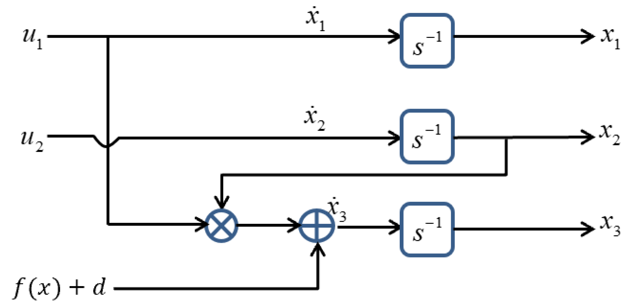
In chained form, the third-order asymmetric nonholonomic robotic system is considered as follows:

$$\begin{array}{l}{\dot{x}}_1=u_1,\\ {\dot{x}}_2=u_2,\\ {\dot{x}}_3=f\left(x\right)+x_2{u}_1+d\end{array}$$

(1)

The vector $x={[x_1,x_2,x_3]}^T$ signifies the state’s variables, $u_1,u_2\in R$ describe the input signals, $d\in R$ is the external disturbance, $f\left(x\right),x_2$ are the nominal terms of the system and $x_2\ne 0$. The nonholonomic model (1) is the third-order equation (with some changes) of the chained-form n-dimensional nonholonomic system, which is described in [25]. The schematic view of the third-order asymmetric nonholonomic system is illustrated in Figure 1. The nonholonomic systems have nonintegrable constraints (see the survey paper [26] and references therein for the introductory examples). The main problem for the asymptotical stability of nonholonomic structures is the uncontrollability of their first-order approximation and non-existence of the smooth (or even continuous) state-feedback controller [27,28].

Assumption 1.

It is assumed that the external disturbance (d) and its time derivative ($\dot{d}$) are bounded functions, and their upper bounds are known.

Suppose that the vector $x_d={[x_{1d},x_{2d},x_{3d}]}^T$ contains some desired responses and is found utilizing the following differential equations [29]:

$$\begin{array}{l}{\dot{x}}_{1d}=u_{1d},\\ {\dot{x}}_{2d}=u_{2d},\\ {\dot{x}}_{3d}=f\left(x_d\right)+x_{2d}{u}_{1d}\end{array}$$

(2)

The variables $u_{1d}$ and $u_{2d}$ are the input signals of the reference model. Let us define the tracking error as $x_e=x-x_d$. Then, the error equations are found as:

$$\begin{array}{l}{\dot{x}}_{1e}=u_1-u_{1d},\\ {\dot{x}}_{2e}=u_2-u_{2d},\\ {\dot{x}}_{3e}=x_{2e}{u}_{1d}+\left(x_{2e}+x_{2d}\right)\left(u_1-u_{1d}\right)+f\left(x\right)-f\left(x_d\right)+d.\end{array}$$

(3)

The main control aim is to synthesize an optimal and robust tracking control law for the asymmetric nonholonomic robotic system (1).

3. Controller Design

The proposed design procedure entails three stages: (i) synthesizing an optimal controller law for the nominal dynamical system, (ii) in the existence of exterior disturbances, an ITSM control law is designed to ensure robustness, and (iii) combining the controllers of (i) and (ii). The overall control input $u_1$ can be written as:

$$u_1=u_{op}+u_2,$$

(4)

where $u_{op}\in R$ is the optimal control input aiming at stabilizing the nominal system, and $u_2\in R$ is the ITSMC law synthesized to ensure the system’s robust performance under the disturbances.

(A) 

Optimal control law design

Define the performance criterion $J$ as:

$$J={{\displaystyle \int }}_0^{\infty }(p\left(x\right)+u_{op}{}^2)dt,$$

(5)

where $p\left(x\right)$ is a positive semi-definite continuously differentiable function, and $\left(f\left(x\right),p\left(x\right)\right)$ is zero-state detectable, with the desired solution as a state-feedback control input. Neglecting the external disturbances in (1) yields:

$$\dot{x}=f\left(x\right)+x_2{u}_{op},$$

(6)

where $x\in R^3$ are the states, and the vector function $f\left(x\right)\in R^3$ has continuous partial derivatives regarding $x$. It is assumed that the pair $\left(f\left(x\right),p\left(x\right)\right)$ is zero-state detectable. So, one can select a CLF to stabilize the nonlinear system and then synthesize a feedback controller $u_{op}$, where the time-derivative of the CLF is a negative-definite function.

The presence of a suitable Lyapunov function for the nonlinear system (6) is a necessary/sufficient condition for the satisfaction of the stability of the system. For stabilization of the nonlinear system (6), it is required to choose a Lyapunov function first and then attempt a feedback control law such that it makes the time-derivative of the Lyapunov function negative definite. The Lyapunov stability satisfies the stability of the nonlinear system without control inputs, and it is employed for the closed-loop control systems. However, the notion of the CLF controller is to find a Lyapunov candidate function for the open-loop system and then design a feedback control loop that constructs the Lyapunov derivative negative. If one can find a suitable CLF, then it is also possible to design an appropriate stabilizer for the nonlinear system.

In the nonlinear system, the CLF-based controller is synthesized by choosing a Lyapunov function. Then, a feedback law is found in such a way that the time-derivative of the Lyapunov candidate becomes a negative one [30]. Accordingly, a stabilizing control input $u_{op}$ would be designed when one can find a CLF. Considering the Lyapunov function $V_1$ as a positive-definite and radially unbounded function, the time derivative of $V_1$ along with the system dynamics (6) is expressed as:

$${\dot{V}}_1=\frac{\partial V_1}{\partial x}\dot{x}=L_f{V}_1+L_{x_2}{V}_1{u}_{op},$$

(7)

where $L_f{V}_1=\frac{\partial V_1}{\partial x}f$, $L_{x_2}{V}_1=\frac{\partial V_1}{\partial x}{x}_2$ and $L$ is the Lie derivative operator. The function $V_1$ is a CLF for any $x\ne 0$, if $L_{x_2}{V}_1=0$ yields $L_f{V}_1<0$.

Using the standard converse theorem, one can conclude that if (6) is stabilizable, a CLF exists. Moreover, if a CLF exists for the system (6), an asymptotically stabilizing controller that stabilizes (6) also exists. For such a nonlinear system, Sontag [16] proposed a CLF-based controller as follows:

$$u_{op}=\{\begin{array}{ll}-\left[\frac{a\left(x\right)+\sqrt{\overline{a}}}{b{(x)}^{T}b\left(x\right)}\right]b{(x)}^T,& b\left(x\right)\ne 0\\ 0,& b\left(x\right)=0\end{array}$$

(8)

with $\overline{a}=a{(x)}^2+p\left(x\right)b{(x)}^{T}b\left(x\right)$ and

$$a\left(x\right)=L_f{V}_1,$$

(9)

$$b\left(x\right)=L_{x_2}{V}_1.$$

(10)

Theorem 1.

The control input$u_{op}$(8) stabilizes the nominal parts of the nonholonomic system (6) and minimizes the performance criterion (5).

Proof. 

Define the HJB equation [31]:

$$L_f{V}_1{}^{*}-\frac{1}{4}{(L_{x_2}{V_1}^{*})}^T{L}_{x_2}{V_1}^{*}+p\left(x\right)=0,$$

(11)

where ${V_1}^{*}$ would be a solution of the HJB equation, with:

$$V_1{}^{*}=\underset{u_{op}}{inf}{{\displaystyle \int }}_t^{\infty }\left(p\left(x\right)+u_{op}{}^2\right)d\tau .$$

(12)

The following optimal control law can be defined [19] if a continuously differentiable and positive-definite solution exists for the HJB equation (11):

$$u^{*}=-\frac{1}{2}{L}_{x_2}{V}_1{}^{*}.$$

(13)

Defining a scalar function $\lambda$ such that $V_1{}^{*}=\lambda V_1$ yields the optimal control law:

$$u^{*}=-\frac{1}{2}{(\lambda L_{x_2}{V}_1)}^T.$$

(14)

Note that $\lambda$ can be specified by substituting $V_1{}^{*}=\lambda V_1$ in (11):

$$\lambda L_f{V}_1-\frac{1}{4}{\lambda }^2{(L_{x_2}{V}_1)}^T{L}_{x_2}{V}_1+p\left(x\right)=0.$$

(15)

Solving (15) and using (9) and (10) yields:

$$\lambda =2\left(\frac{a\left(x\right)+\sqrt{a{(x)}^2+p\left(x\right)b{(x)}^{T}b\left(x\right)}}{b{(x)}^{T}b\left(x\right)}\right).$$

(16)

Substituting (16) into (14) yields the control law $u^{*}$, defined by:

$$u^{*}=-\left[\frac{a\left(x\right)+\sqrt{a{(x)}^2+p\left(x\right)b{(x)}^{T}b\left(x\right)}}{b{(x)}^{T}b\left(x\right)}\right]b{(x)}^T.$$

(17)

Then, the control law $u^{*}$ is equal to the optimal controller $u_{op}$ presented in Sontag’s formula (8). Thereby, $u_{op}$ minimizes the performance index (5). □

Remark 1.

Considering (7) and replacing$u_{op}$by (8), using the CLF property, i.e.,$L_f{V}_1<0$when$L_{x_2}{V}_1=0$, it can be determined that${\dot{V}}_1$is negative for$u_{op}=0$. On the other hand, for$u_{op}\ne 0$, one can obtain from (7) and (8) that:

$${\dot{V}}_1=-\sqrt{a{(x)}^2+p\left(x\right)b{(x)}^2}<-\left|\sqrt{a{(x)}^2+p\left(x\right)b{(x)}^2}\right|<0.$$

(18)

Thus, it is verified that the control law (8) minimizes the criterion (5) and stabilizes the nominal system (6).

Remark 2.

A necessary condition for CLF-based optimal control design is the full knowledge about the system under consideration. Thus, the effectiveness of the optimal controller degrades when systems are affected by perturbations in the vicinity of the equilibrium.

To circumvent this problem, one can combine the aforementioned optimal control design with an SMC approach to guarantee robustness under external disturbances.

(B) 

ITSMC control design

In what follows, we propose suppressing the disturbances affecting the nonlinear system (1) via an ITSMC design and then incorporating both control inputs into a switching controller.

We define the recursive TSM structure as

$$\begin{array}{l}{\sigma }_1=x_{2e}+x_{3e}=0,\\ {\sigma }_2={\dot{\sigma }}_1+{\rho }_1{\sigma }_1{}^{p_1/q_1}=0,\\ {\sigma }_3={\dot{\sigma }}_2+{\rho }_2{\sigma }_2{}^{p_2/q_2}=0,\end{array}$$

(19)

The constants $q_i$ and $p_i$, $p_i<q_i$ and ${\rho }_i$ $\left(i=1,2\right)$ are some positive odd integers. The terms ${\sigma }_i$’s $\left(i=1,2,3\right)$ are the TSM surfaces.

Taking the time derivative of ${\sigma }_i$ $\left(i=1,2,3\right)$, we have:

$$\begin{array}{l}{\dot{\sigma }}_1={\dot{x}}_{2e}+{\dot{x}}_{3e}=u_2-u_{2d}+x_{2e}{u}_{1d}+f\left(x\right)-f\left(x_d\right)+d,\\ {\dot{\sigma }}_2={\ddot{\sigma }}_1+{\rho }_1\frac{d}{dt}\left({\sigma }_1{}^{p_1/q_1}\right),\\ {\dot{\sigma }}_3={\ddot{\sigma }}_2+{\rho }_2\frac{d}{dt}\left({\sigma }_2{}^{p_2/q_2}\right).\end{array}$$

(20)

Thus, the finite-time convergence property of the TSM implies that the switching surfaces ${\sigma }_1$, ${\sigma }_2$, and ${\sigma }_3$ would reach zero in finite time. Considering the reachability condition of a conventional ISM, one has

$${\dot{\sigma }}_1<-\rho sgn({\sigma }_1),$$

(21)

where $\rho >0$ and the function $sgn({\sigma }_1)$ are defined as:

$$sgn({\sigma }_1)=\{\begin{array}{ll}1,& {\sigma }_1>0\\ 0,& {\sigma }_1=0\\ -1.& {\sigma }_1<0\end{array}$$

(22)

and using (20) and (21), it yields:

$$u_2<u_{2d}-x_{2e}{u}_{1d}-f\left(x\right)+f\left(x_d\right)-d-\rho sgn({\sigma }_1).$$

(23)

The existence of the sign function in the switching controller $u_2$ implies that the chattering phenomenon is unavoidable. One way to circumvent this problem is by considering the nonsingular terminal sliding manifold $\kappa$ [32,33]:

$$\kappa ={\sigma }_1+\delta {\dot{\sigma }}_1{}^{\alpha /\beta },$$

(24)

where $\alpha$ and $\beta$ with $1<\frac{\alpha }{\beta }<2$ are positive odd integers, $\delta$ is the positive switching gain and ${\sigma }_1$ is the integral sliding surface. Using (20), one obtains:

$${\dot{\sigma }}_1=u_2-u_{2d}+x_{2e}{u}_{1d}+f\left(x\right)-f\left(x_d\right)+d=u_2+\zeta +d,$$

(25)

where $\zeta =-u_{2d}+x_{2e}{u}_{1d}+f\left(x\right)-f\left(x_d\right)$. An improved reaching condition for the nonsingular terminal sliding manifold $\kappa$ is proposed as follows:

$$\dot{\kappa }=-{\eta }_{1}sgn\left(\kappa \right)-{\epsilon }_1\kappa ,$$

(26)

where ${\eta }_1>0$ and ${\epsilon }_1>0$.

Computing the derivative of the terminal sliding surface (24) gives:

$$\begin{array}{l}\dot{\kappa }={\dot{\sigma }}_1+\delta \frac{\alpha }{\beta }{\dot{\sigma }}_1{}^{\alpha /\beta -1}{\ddot{\sigma }}_1\\ =\delta \frac{\alpha }{\beta }{\dot{\sigma }}_1{}^{\alpha /\beta -1}\left(\frac{\beta }{\delta \alpha }{\dot{\sigma }}_1{}^{2-\alpha /\beta }+{\ddot{\sigma }}_1\right).\end{array}$$

(27)

From the positiveness of the odd parameters $\alpha$ and $\beta$, it can be shown that:

$$\begin{array}{l}{\dot{\sigma }}_1{}^{\alpha /\beta -1}>0,for{\dot{\sigma }}_1\ne 0\\ {\dot{\sigma }}_1{}^{\alpha /\beta -1}=0. for {\dot{\sigma }}_1=0,\end{array}$$

(28)

Furthermore, from (27) and (28), the term $\delta (\alpha /\beta ){\dot{\sigma }}_1{}^{\alpha /\beta -1}$ in (27) can be replaced by the new positive variable ${\eta }_2>0$ for ${\dot{\sigma }}_1\ne 0$. Hence, Equation (27) can be written as:

$$\dot{\kappa }={\eta }_2(\frac{\beta }{\delta \alpha }{\dot{\sigma }}_1{}^{2-\alpha /\beta }+{\ddot{\sigma }}_1).$$

(29)

Equaling the values of $\dot{\kappa }$ from (26) and (29) can be expressed as:

$$\frac{\beta }{\delta \alpha }{\dot{\sigma }}_1{}^{2-\alpha /\beta }+{\ddot{\sigma }}_1=-\eta sgn(\kappa )-\epsilon \kappa ,$$

(30)

where $\eta ={\eta }_1/{\eta }_2>0$ and $\epsilon ={\epsilon }_1/{\eta }_2>0$ and $\epsilon$ is a parameter selected to define the convergence rate of the sliding surface. Then, Equation (30) can be rewritten as:

$${\ddot{\sigma }}_1=-\eta sgn(\kappa )-\epsilon \kappa -\frac{\beta }{\delta \alpha }{\dot{\sigma }}_1{}^{2-\alpha /\beta }.$$

(31)

Differentiating (25) with respect to time gives rise to:

$${\ddot{\sigma }}_1={\dot{u}}_2+\dot{\zeta }+\dot{d}.$$

(32)

Using (31) and (32) yields the following switching controls:

$$u_2=-{{\displaystyle \int }}_0^t\left[\eta sgn(\kappa )+\epsilon \kappa +\frac{\beta }{\delta \alpha }{\dot{\sigma }}_1{}^{2-\alpha /\beta }+\dot{\zeta }+\mu sgn\left(\kappa \right)\right]d\tau .$$

(33)

where $\mu \ge \left|\dot{d}\right|$.

Theorem 2.

The finite-time convergence of the nonlinear system (1) would be ensured by selecting the terminal sliding manifold (24) and designing the control law:

$$u_1=u_{op}+u_2,$$

(34)

where $u_{op}$ and $u_2$ are defined as

$$u_{op}=\{\begin{array}{ll}-\left[\frac{a(x)+\sqrt{a{(x)}^2+p(x)b{(x)}^{T}b(x)}}{b{(x)}^{T}b(x)}\right]b{(x)}^T,& b(x)\ne 0\\ 0& b(x)=0\end{array}$$

(35)

$$u_2=-{{\displaystyle \int }}_0^t\left[\left(\eta +\mu \right)sgn(\kappa )+\epsilon \kappa +\frac{\beta }{\delta \alpha }{\dot{\sigma }}_1{}^{2-\alpha /\beta }+\dot{\zeta }\right]d\tau$$

(36)

with $\mu \ge \left|\dot{d}\right|$.

Proof. 

In order to prove the convergence of the nonsingular terminal sliding manifold $\kappa$, the Lyapunov candidate function is defined as:

$$V_2=\frac{1}{2}{\kappa }^2$$

(37)

Differentiating $V_2$ yields:

$${\dot{V}}_2=\kappa \dot{\kappa }.$$

(38)

Substituting (27) and (32) into (38) yields:

$$\begin{array}{ll}{\dot{V}}_2& =\kappa \left[{\dot{\sigma }}_1+\frac{\alpha \delta }{\beta }{\dot{\sigma }}_1{}^{\alpha /\beta -1}{\ddot{\sigma }}_1\right]\\ & =\kappa \left[{\dot{\sigma }}_1+\frac{\alpha \delta }{\beta }{\dot{\sigma }}_1{}^{\alpha /\beta -1}({\dot{u}}_2+\dot{\zeta }+\dot{d})\right].\end{array}$$

(39)

From (33), one can obtain:

$$\begin{array}{ll}{\dot{V}}_2=\kappa & \left[{\dot{\sigma }}_1+\frac{\alpha \delta }{\beta }{\dot{\sigma }}_1{}^{\alpha /\beta -1}\left(-\eta sgn(\kappa )-\epsilon \kappa -\frac{\beta }{\delta \alpha }{\dot{\sigma }}_1{}^{2-\alpha /\beta }-\dot{\zeta }-\mu sgn\left(\kappa \right)+\dot{\zeta }+\dot{d}\right)\right]\\ & \le \kappa \left[\frac{\alpha \delta }{\beta }{\dot{\sigma }}_1{}^{\alpha /\beta -1}\left(-\eta sgn(\kappa )-\epsilon \kappa \right)\right]-\frac{\alpha \delta }{\beta }{\dot{\sigma }}_1{}^{\alpha /\beta -1}(\mu \left|\kappa \right|-\left|\dot{d}\right|\left|\kappa \right|)\\ & \le \frac{\alpha \delta }{\beta }{\dot{\sigma }}_1{}^{\alpha /\beta -1}\left[-\eta \left|\kappa \right|-\epsilon {\kappa }^2\right],\end{array}$$

(40)

whereas $\delta >0$ and $1<\alpha /\beta <2$, it follows that ${\dot{\sigma }}_1{}^{\alpha /\beta -1}>0$ for any ${\dot{\sigma }}_1\ne 0$ and ${\dot{\sigma }}_1{}^{\alpha /\beta -1}=0$ only for ${\dot{\sigma }}_1=0$. Hence, it is concluded from (40) that:

$$\begin{array}{l}{\dot{V}}_2\left(\kappa \right)\le -{\eta }_2[\epsilon {\left|\kappa \right|}^2+\eta \left|\kappa \right|]\\ \le -\overline{\alpha }V\left(\kappa \right)-\overline{\beta }V{(\kappa )}^{\overline{\eta }}<0,\end{array}$$

(41)

where $\overline{\eta }=1/2$, $\overline{\alpha }=2{\eta }_2\epsilon$ and $\overline{\beta }=\sqrt{2}{\eta }_2\eta$. Thus, it is confirmed that the terminal sliding manifold $\kappa$ would be converged to zero in finite time for any initial condition. Subsequently, the tracking error convergence to the origin would be guaranteed in finite time for the nonlinear system (1). □

4. Computer Simulations

Wheeled mobile robots are progressively used in industrial robotic systems, especially when an autonomous motion is required for smooth surfaces. Most of the considered models of wheeled mobile robots are in accordance with the laboratory-scale mobile robots that have a light weight. For this purpose, the dynamics of the wheeled mobile robots are ignored, and only the kinematics of these robots are usually considered. The kinematics of a wheeled mobile robot is a simplified model and does not correspond to the reality of the moving vehicle, which obtains time-varying unknown mass and friction [34]. The stabilization/tracking control of nonholonomic wheeled mobile robots with motion restrictions is, in general, challenging. The control of nonholonomic wheeled mobile robots cannot be implemented by the linear control techniques, and the dynamic equations of these systems cannot be transformed into the linear control system structures. The design of the control law using the dynamical model of wheeled mobile robots, where parametric uncertainties in the physical parameters are obviously considered, stimulates researchers to investigate this field [35]. Actually, because of both the richness and hardness of dynamics of wheeled mobile robots, such nonlinear control systems have interested researchers in studying various control methods.

The suggested optimal integral finite-time control approach is implemented on the wheeled mobile robot, with its equations represented by:

$$\begin{array}{l}{\dot{x}}_1=u_1,\\ {\dot{x}}_2=u_2,\\ {\dot{x}}_3=x_1+x_2^2+x_3+x_2{u}_1+sin(0.1\pi t),\end{array}$$

(42)

The nonlinear function and disturbance are $f\left(x\right)=x_1+x_2^2+x_3$ and $d=sin(0.1\pi t)$, for which we define the following state and control transformations [25]:

$$\begin{array}{l}{x}_1=\theta \\ x_2=-xsin \theta +ycos \theta \\ x_3=xcos \theta +ysin \theta \\ {\dot{u}}_1=w_2\\ {\dot{u}}_2=w_1-\left(xcos \theta +ysin \theta \right)w_2\end{array}$$

(43)

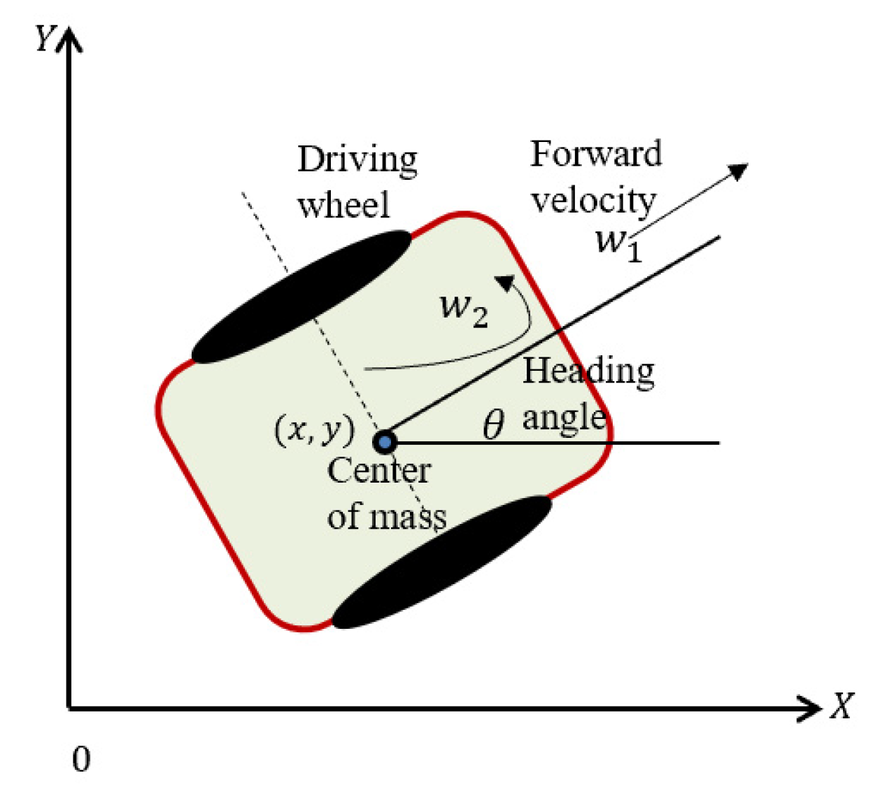
where $x$ and $y$ are locations of the center of mass (CAM), $\theta$ represents the heading angle, $w_1$ is the forward velocity of the CAM, and $w_2$ is the angular velocity.

A schematic view of the considered wheeled mobile robot is shown in Figure 2.

The reference model is taken as:

$$\begin{array}{l}{\dot{x}}_{1d}=u_{1d},\\ {\dot{x}}_{2d}=u_{2d},\\ {\dot{x}}_{3d}=f\left(x_d\right)+x_{2d}{u}_{1d},\end{array}$$

(44)

The nonlinear term is selected as $f\left(x_d\right)=x_{1d}+x_{2d}^2+x_{3d}$, and we Define the tracking errors $x_{ie}=x_i-x_{id}\left(i=1,2,3\right)$ such that:

$$\begin{array}{l}{\dot{x}}_{1e}=u_1-u_{1d},\\ {\dot{x}}_{2e}=u_2-u_{2d},\\ {\dot{x}}_{3e}=x_{2e}{u}_{1d}+\left(x_2\right)\left(u_1-u_{1d}\right)+f\left(x\right)-f\left(x_d\right)+d.\end{array}$$

(45)

To evaluate the closed-loop performance, the required parameters are selected as: $\beta =1$, $\epsilon =0.001$, $p_1=1$, $q_1=1$, $p_2=5$, $q_2=5$, ${\rho }_1=1$, ${\rho }_2=1$, $\alpha =2$, $\eta =0.1$, $\delta =-1$ and $\mu =0.1$. The initial states are $x_e\left(0\right)=\left[1,0,-1\right]$, $u_1\left(0\right)=-2$, $u_2\left(0\right)=2$. The input signals of the reference model are taken as $u_{1d}=e^{-t}$, and $u_{2d}=e^{-2t}$. The performance criterion $J$ is considered as $J={{\displaystyle \int }}_0^{\infty }(x^T{I}_{3}x+u_{op}{}^2)dt,$ where $x=\left[x_1,x_2,x_3\right]$, and $I_3$ is the $3\times 3$ identity matrix. The function $p\left(x\right)$ is $p\left(x\right)=\left[x_1,x_2,x_3\right]\left[\begin{array}{ccc}1& 0& 0\\ 0& 1& 0\\ 0& 0& 1\end{array}\right]\left[\begin{array}{c}{x}_1\\ x_2\\ x_3\end{array}\right]$. The control Lyapunov function is defined by $V_1=\frac{1}{2}\left(x_1^2+x_2^2+x_3^2\right)$. The functions $a\left(x\right)$ and $b\left(x\right)$ are $a\left(x\right)=x_3\left(x_1+x_2^2+x_3\right)$ and $b\left(x\right)=x_1-x_2{x}_3$. Then, it yields the CLF-based suboptimal controller defined by:

$$u_{op}=\{\begin{array}{ll}-\left[\frac{x_3\left(x_1+x_2^2+x_3\right)+\sqrt{\varphi }}{{\left(x_1-x_2{x}_3\right)}^2}\right]\left(x_1-x_2{x}_3\right),& b\left(x\right)\ne 0\\ 0,& b\left(x\right)=0\end{array}$$

(46)

where $\varphi =x_3{}^2{\left(x_1+x_2^2+x_3\right)}^2+\left(x_1^2+x_2^2+x_3^2\right){\left(x_1-x_2{x}_3\right)}^2$. Moreover, the overall control law is defined as:

$$\begin{array}{l}{u}_1=u_{op}+u_2\\ =-\left[\frac{x_3\left(x_1+x_2^2+x_3\right)+\sqrt{\varphi }}{{\left(x_1-x_2{x}_3\right)}^2}\right]\left(x_1-x_2{x}_3\right)-{{\displaystyle \int }}_0^t\left[\left(\eta +\mu \right)sgn(\kappa )+\epsilon \kappa -\frac{\beta }{\delta \alpha }{\dot{\sigma }}_1{}^{2-\alpha /\beta }+\dot{\zeta }\right]d\tau .\end{array}$$

(47)

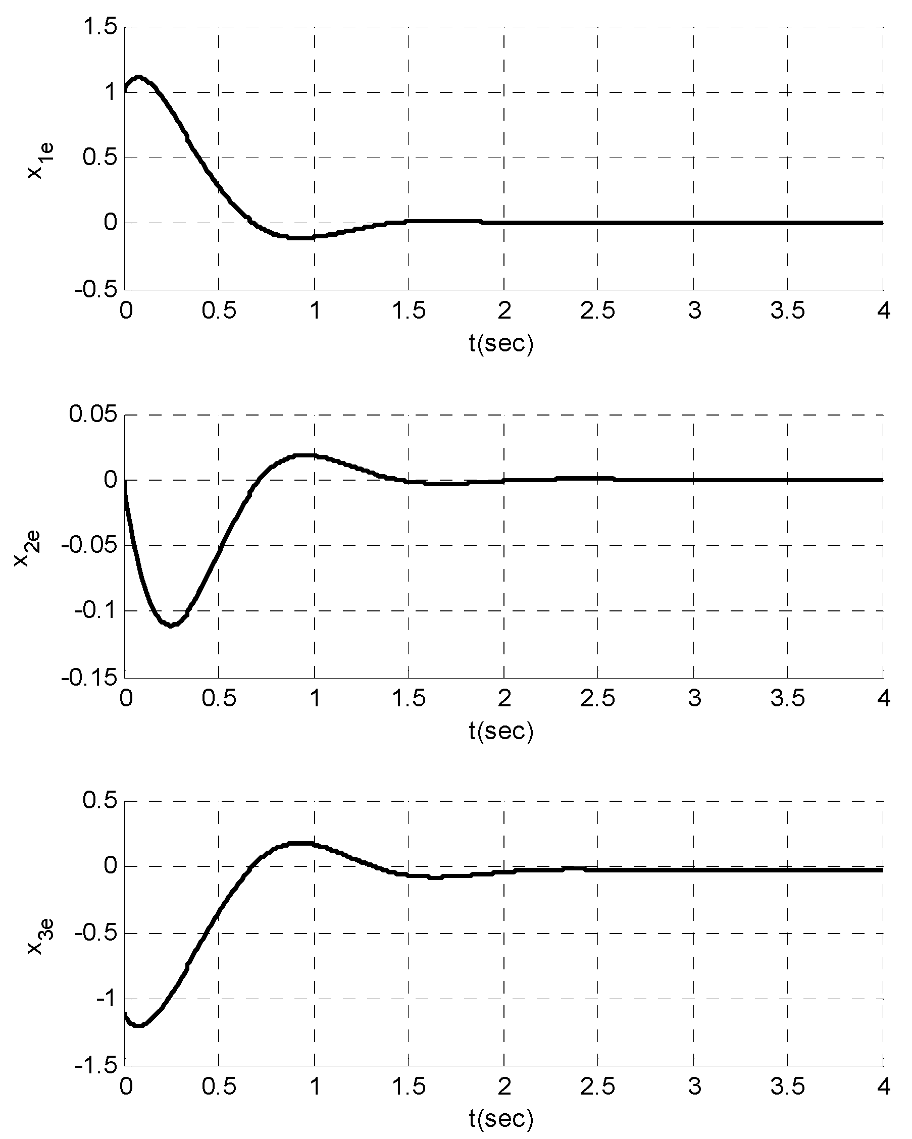
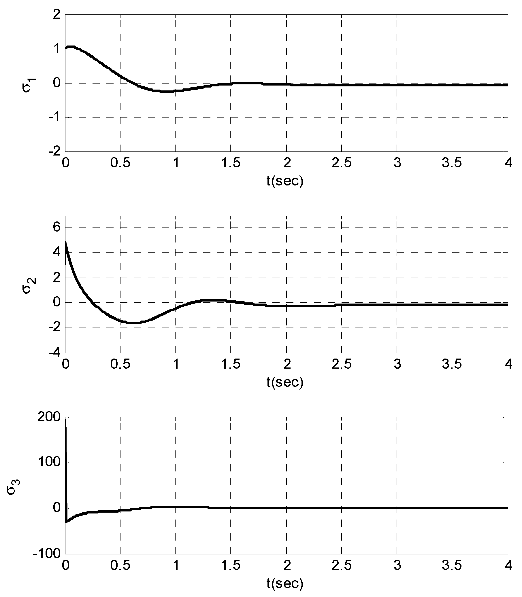
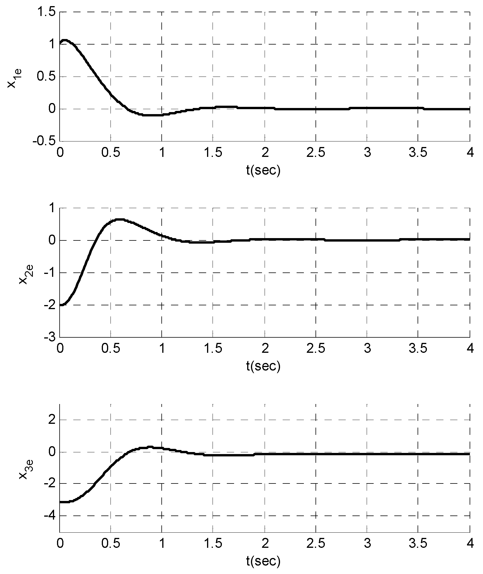
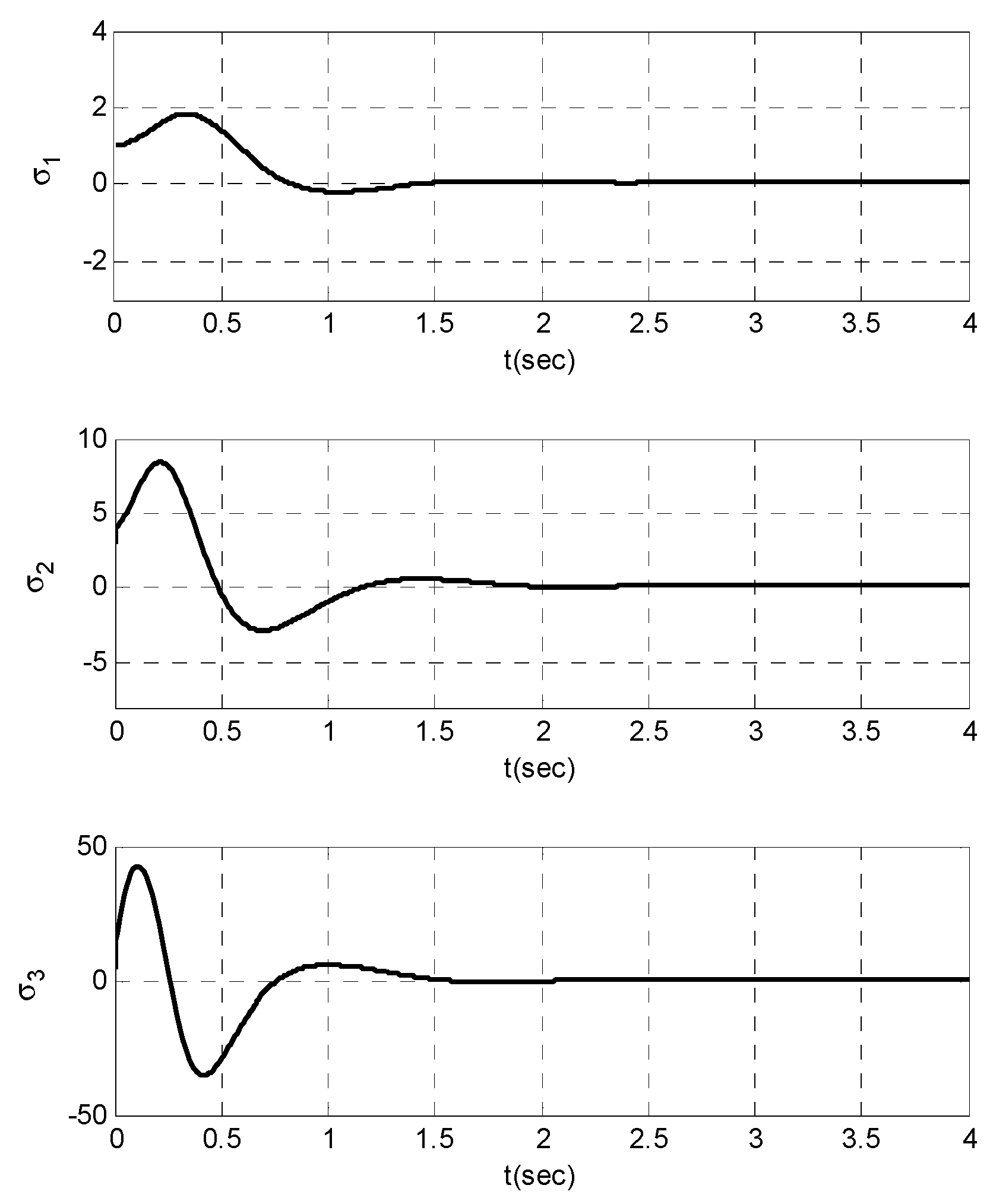
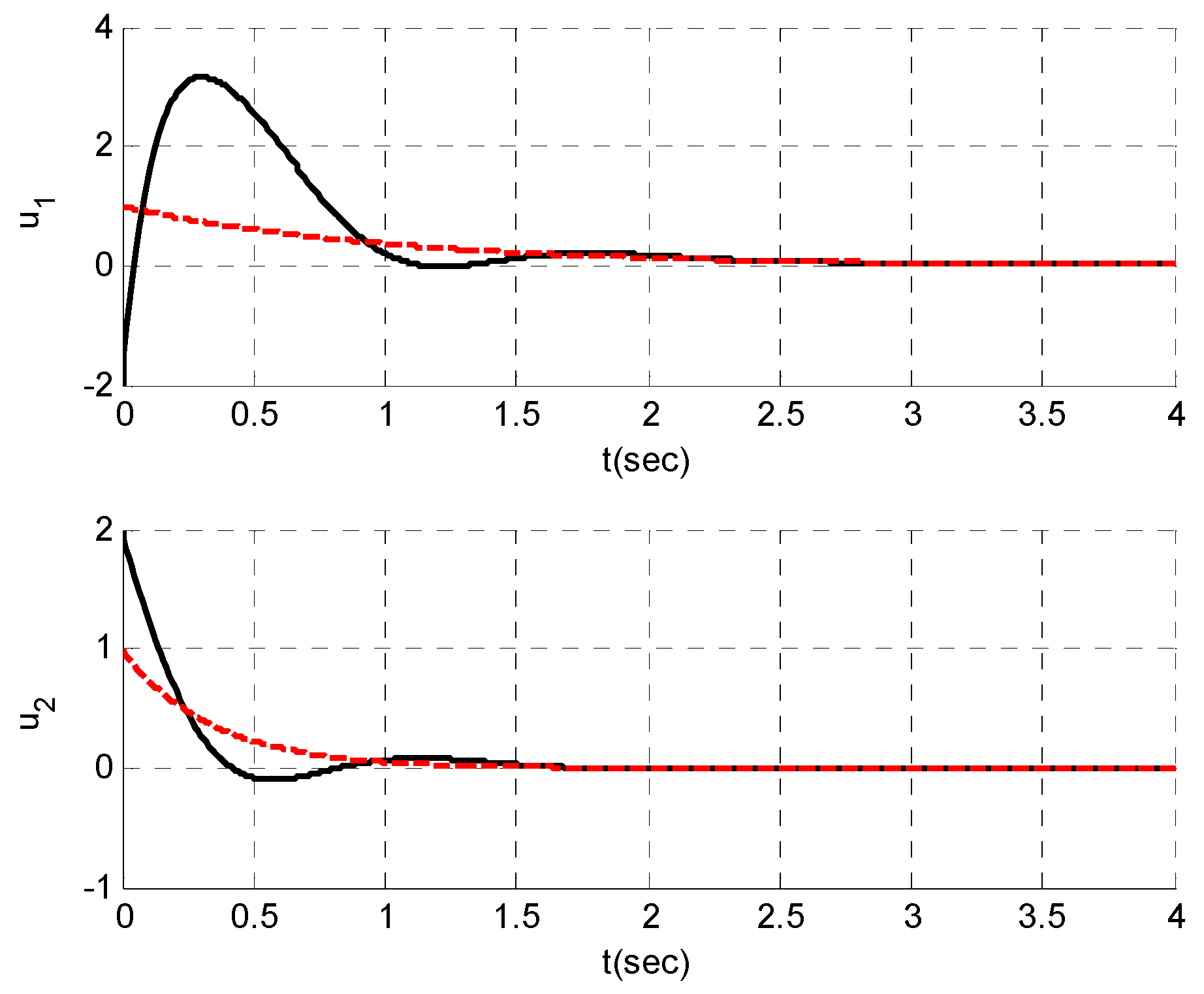
Figure 3 depicts the dynamics of the error signals. Note that this figure illustrates the superior tracking performance and robustness of the responses in the presence of external disturbances. The sliding surfaces are exposed in Figure 4, which demonstrates the quick convergence of the sliding surfaces to the origin. The dynamics of the control efforts $u_1$ and $u_2$ and the trajectories of the desired control inputs are depicted in Figure 5. It is shown that the control inputs are smooth and are able to overcome the nonlinearities and external disturbances. As a result, it can be observed from these figures that the proposed control method can satisfy the superior tracking responses in the existence of external disturbances.

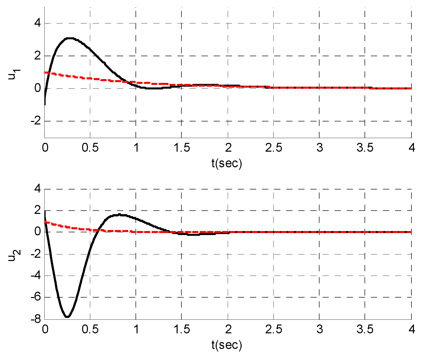
For the robustness analysis, the initial conditions of the tracking errors and control inputs are considered as $x_e\left(0\right)=\left[1,-2,-3\right]$, $u_1\left(0\right)=-1$, and $u_2\left(0\right)=2$. The external disturbance term is set as $d=0.3sin(0.2\sqrt{0.5t})$. Time responses of the tracking errors, switching surfaces, and control input signals are shown in Figure 6, Figure 7 and Figure 8. It can be seen from Figure 6 that the tracking errors converge to the origin suitably, without any steady-state error. Moreover, it can be seen from Figure 7 and Figure 8 that the sliding surfaces and control inputs converge to zero without any chattering problem. All of the results exhibit that the responses are robust in the new condition, with different initial states and external disturbance values.

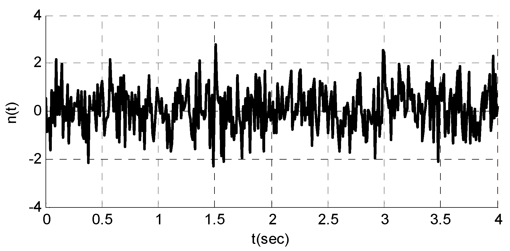
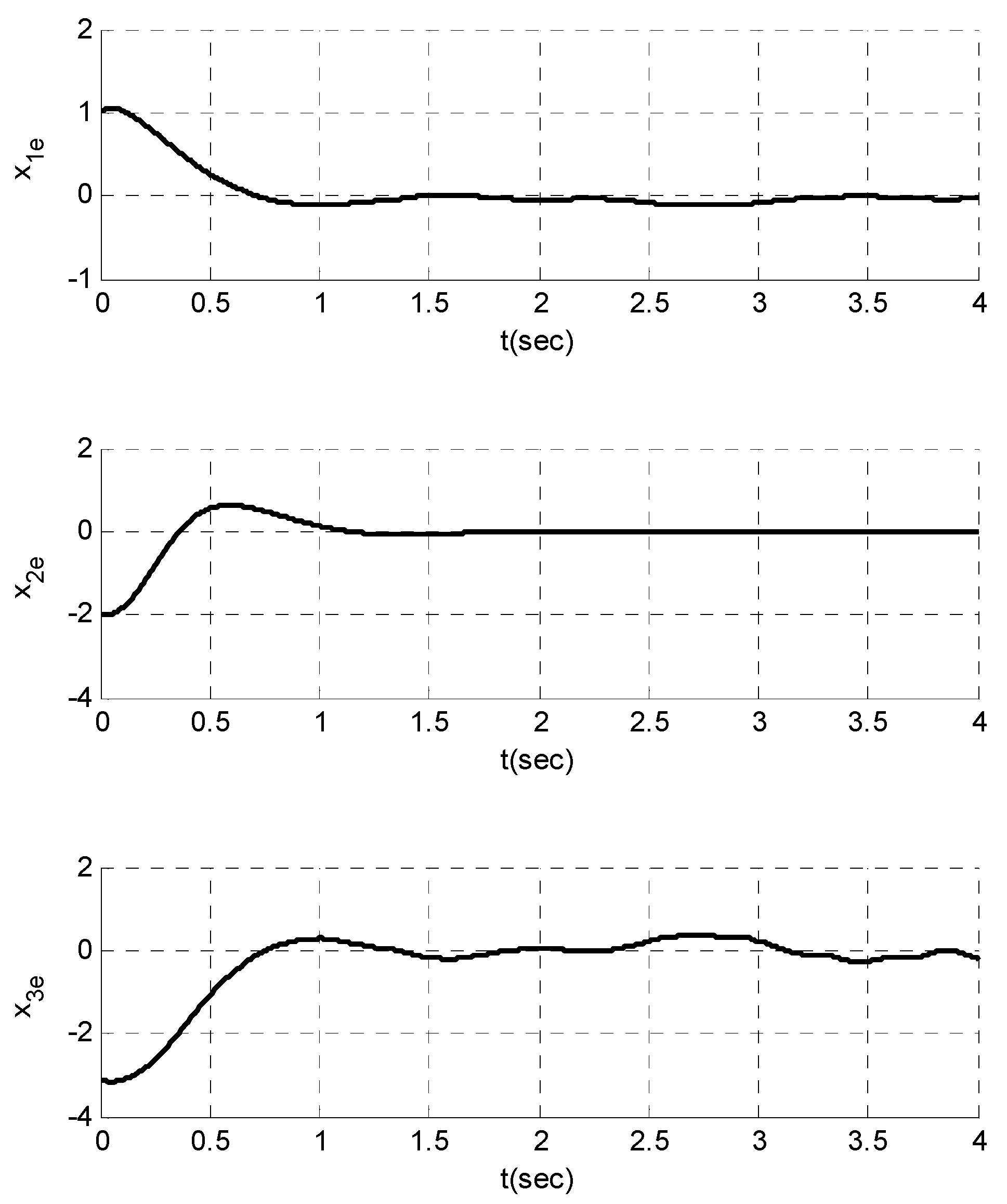
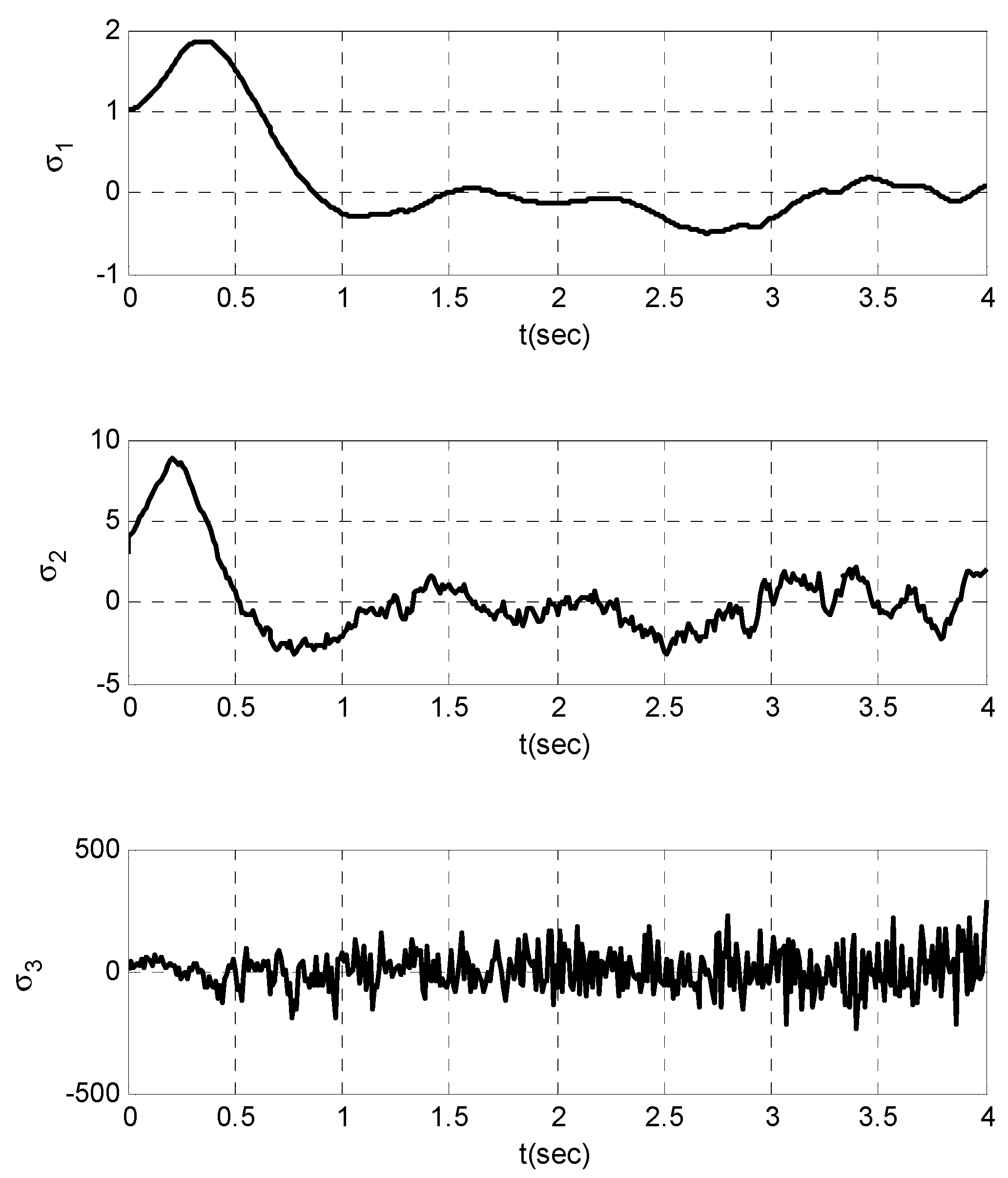
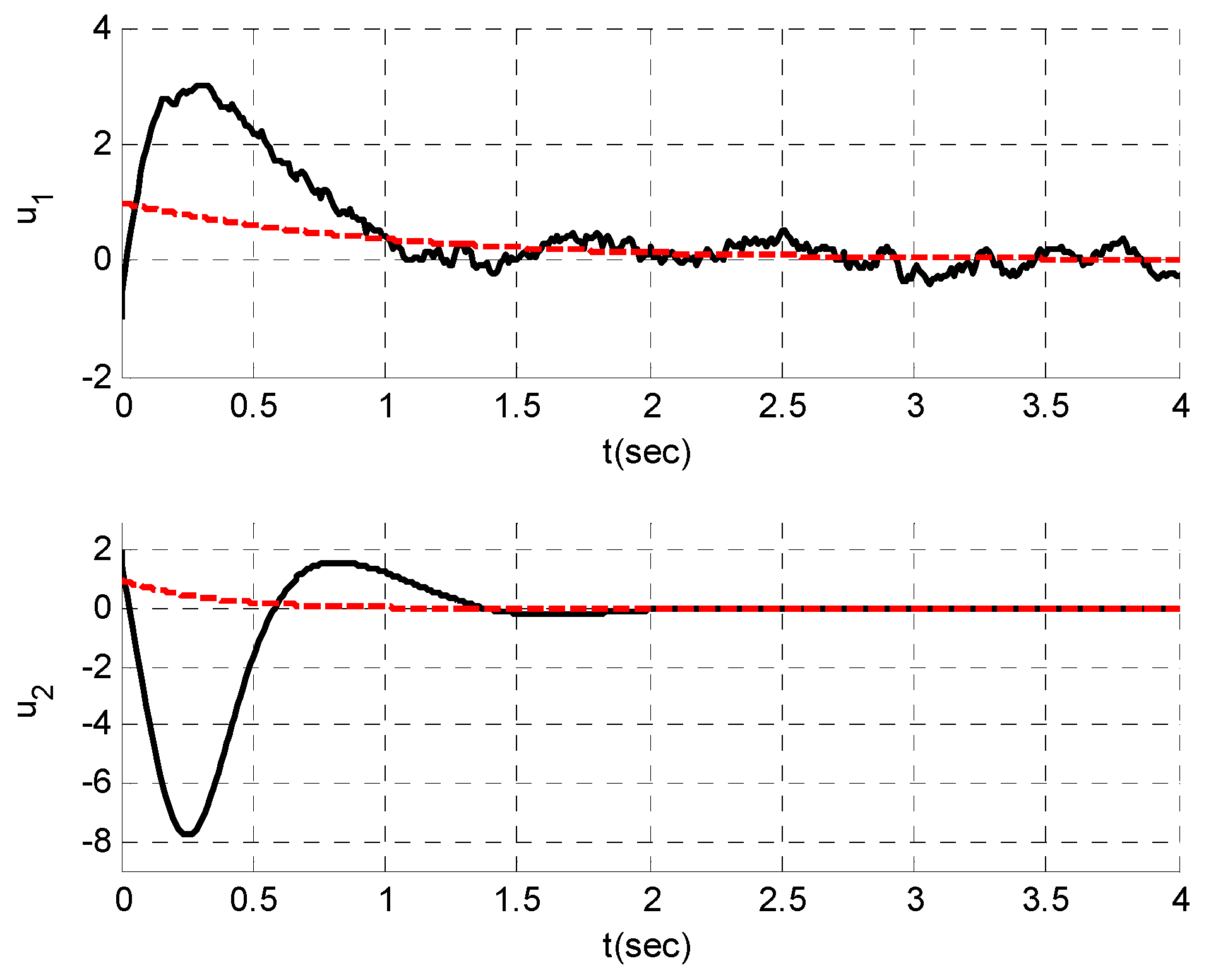
For more studies on the robustness of the control method, a band-limited white noise (with noise power 0.001, sample time 1 millisecond) is added to the states of the system. Figure 9 shows the measurement noise signal. This noise signal shows that the responses of the system seem somewhat noisy. Time responses of the tracking errors, sliding surfaces, and control inputs are shown in Figure 10, Figure 11 and Figure 12. In the time responses of Figure 10, it can be seen that the tracking error signals are convergent to the origin. However, these responses experience some light effects of measurement noises. Furthermore, the noisy responses can be observed in the sliding surfaces (Figure 11) and control inputs (Figure 12); nevertheless, the sliding surfaces and control signals oscillate around zero, which shows that the responses do not diverge to infinity (the responses remain stable). Hence, the advised control method has acceptable robust performance in the existence of exterior disturbances and measurement noise.

5. Conclusions

A control Lyapunov-based optimal integral terminal sliding mode control approach is planned for a class of asymmetric nonholonomic robotic systems with external disturbances. The design procedure entailed synthesizing an optimal control law based on the CLF for the nominal system, then deriving an ITSMC approach to ensure robustness against modelled and unmodelled disturbances. To ensure both finite-time stability and robustness, the optimal control input is combined with the integral TSM. Apart from the robustness features, the suggested methodology has the benefit of being optimum and chattering-free, thereby being better suited for practical implementations to common systems, such as surface vessels, wheeled robots, space crafts, etc. For the extension of the proposed work, the event-triggered optimal finite-time tracking controller design method for perturbed nonholonomic robotic systems will be considered in future research.