Article

Analysis of Transient Thermal Distribution in a Convective–Radiative Moving Rod Using Two-Dimensional Differential Transform Method with Multivariate Pade Approximant

by
Ganeshappa Sowmya
1,
Ioannis E. Sarris
2,*,
Chandra Sen Vishalakshi
3,
Ravikumar Shashikala Varun Kumar
4 and
Ballajja Chandrappa Prasannakumara
4
1
Department of PG Mathematics, The National College (Auto), Bangalore 560070, India
2
Department of Mechanical Engineering, University of West Attica, 12244 Athens, Greece
3
Department of PG Mathematics, Government Science College, Chitradurga 577501, India
4
Department of Studies and Research in Mathematics, Davangere University, Davangere 577002, India
*
Author to whom correspondence should be addressed.
Symmetry 2021, 13(10), 1793; https://doi.org/10.3390/sym13101793
Submission received: 21 August 2021 / Revised: 18 September 2021 / Accepted: 22 September 2021 / Published: 26 September 2021
(This article belongs to the Special Issue Solid Mechanics and Mechanical Mechanics)

Abstract

:
The transient temperature distribution through a convective-radiative moving rod with temperature-dependent internal heat generation and non-linearly varying temperature-dependent thermal conductivity is elaborated in this investigation. Symmetries are intrinsic and fundamental features of the differential equations of mathematical physics. The governing energy equation subjected to corresponding initial and boundary conditions is non-dimensionalized into a non-linear partial differential equation (PDE) with the assistance of relevant non-dimensional terms. Then the resultant non-dimensionalized PDE is solved analytically using the two-dimensional differential transform method (2D DTM) and multivariate Pade approximant. The consequential impact of non-dimensional parameters such as heat generation, radiative, temperature ratio, and conductive parameters on dimensionless transient temperature profiles has been scrutinized through graphical elucidation. Furthermore, these graphs indicate the deviations in transient thermal profile for both finite difference method (FDM) and 2D DTM-multivariate Pade approximant by considering the forced convective and nucleate boiling heat transfer mode. The results reveal that the transient temperature profile of the moving rod upsurges with the change in time, and it improves for heat generation parameter. It enriches for the rise in the magnitude of Peclet number but drops significantly for greater values of the convective-radiative and convective-conductive parameters.

1. Introduction

The heat transfer process has become one of the important topics in the research domain. Numerous researchers showed their interest in enhancing the heat transfer rate due to the design of heat transfer apparatus crucial for emerging industries and their applications in the engineering field and technological areas. Firstly, this phenomenon was witnessed in the condensers for power generation plants and steam generators for tank engines. Later on, heat exchangers heat transfer process and practice can be found in the petroleum and petrochemical industries. More precisely, the heat transfer process is witnessed in welding, thermosyphons, electronic packaging, nuclear reactors, buildings, geophysics, casting, and food processing. Heat transfer can be occurred by convection, conduction, and radiation. The convection process causes heat transfer in the presence of liquid flow due to the movement of the liquid. In contrast, the radiation and conduction heat transfer are generally seen in extended surfaces (fins, spines, and pins) and solid materials (plates, rods, discs, etc.). Numerous investigators examined the method for enhancing the heat transfer rate. They found that using the special kinds of liquids, namely nanofluid and hybrid nanoliquid consisting of minute nanomaterials, can offer a higher heat transfer rate than the base fluid. As a result, many researchers have scrutinized the heat transfer features in the presence of nanoliquids and hybrid nanoliquids. Recently, Khan et al. [1] explained the heat transference of nanoliquid with magnetic dipole impact past a curvy surface. Tassaddiq [2] inspected micropolar liquid’s heat transfer and flow behavior with hybrid nanomaterials past an elongating geometry by considering the ohmic heating effect. Kumar et al. [3] conferred the heat transferal of a Casson nanoliquid stream past a curvy elongating sheet with an exponential heat source. Wahid et al. [4] debriefed the heat transfer process of a hybrid nanoliquid over a curved elongating geometry, and they talked about the nature of stability analysis and dual branch solutions. Yusuf et al. [5] probed the heat transfer phenomenon and stream of a Williamson nanoliquid past an inclined plate by considering the magnetic impact. Mabood et al. [6] explained the radiative heat transference aspects and flow of a rate-type hybrid nanoliquid past a stretching surface. Using nanomaterials to enhance the convective heat transfer during the fluid flow will be fruitful for large-scale manufacturing industries in obtaining a high heat transfer rate. An alternative way to achieve a high heat transfer rate is to increase the surface area of the material by attaching the extended surface to the primary surface. The surface area required for heat transfer can be increased by attaching the extended surface, and thus the heat is conducted through the extended surface. In addition, the heat is lost to the environment by convection and radiation. In connection to this, several inspections on the heat transfer phenomenon through an extended surface with radiation, convection, and internal heat production have been manifested by numerous researchers. Dogonchi and Ganji [7] clarified the thermal attribute of a convective-radiative moving fin with an internal heat source. Madhura et al. [8] probed the influence of magnetic effect on the thermal gradient of a permeable fin with radiation impact. Sun and Li [9] examined the temperature distribution and one-dimensional heat transference of a straight fin with the power-law function of thermal properties. Das and Kundu [10] debriefed the impact of the electromagnetic effect in the heat transference process of a permeable fin. The heat transfer through a continuous moving material has become an important research topic in recent years. Continuous moving surfaces are associated with significant applications such as casting, extrusion of plastics, hot rolling, and drawing of wires in which a material transfers heat with the ambient while moving through a furnace or a channel. The material’s velocity can be exceptionally slow in some cases, such as crystal growth, or fast in other processes, such as optical fiber drawing. When a high-temperature material exits from a furnace or a die, it is subjected to a colder environment, causing a transient conduction process with surface heat dissipation. With the progression of time, the initial transient in the slow-moving material begins to fade, and the mechanism gradually falls into a steady state. On the other side, the temperature distribution may keep evolving with time throughout the thermal treatment procedure for a quick-moving material. For such moving materials, heat transfer coefficients for convection are significant in the thermal transport process. The temperature distribution in the moving material is then estimated using a mathematical model that provides an energy balance involving heat conduction, heat convection, surface heat dissipation, and internal heat source. In the perspective of this, many investigators inspected the heat transfer and thermal distribution through a moving plate, sheet, or rod from recent years. Choudhury and Jaluria [11] examined the thermal distribution within a rod subjected to surface heat transference, and they obtained the analytical solution in terms of infinite series. Aziz and Lopez [12] inspected the thermal performance of a conductive–radiative moving rod with variable thermal conductivity. Sun et al. [13] employed the spectral collocation method for examining the thermal behavior of moving rod with convective and radiative heat transfer. Sarwe et al. [14] expounded the heat transference and flow of Casson hybrid nanoliquid past a plate moving vertically with a magnetic effect.
The symmetrical problem of boundary conditions is one of the most important concerns in the modelling of fluid dynamics of many kinds of fluid via porous media. Well boundary conditions, axisymmetric boundary conditions, and symmetric boundary conditions are all symmetry problems that should be considered in fluid dynamics. In the current study we have considered convective heat transfer. The heat transfer is improved due to internal heat production and the temperature distribution augments due to additional heat energy. Many investigators examined the heat transfer and thermal performance of fins, disks, and other materials with internal heat production. Onyejekwe et al. [15] delineated the impact of temperature-dependent internal heat generation within a straight fin considering temperature-dependent thermal conductivity. Kezzar et al. [16] conferred internal heat production and thermal distribution through a straight fin by considering the thermal conductivity. Majhi and Kundu [17] evaluated the internal heat production and explained the thermal distribution within an annular disk. Considering heat generation impact, Venkitesh and Mallick [18] probed the thermal behavior of annular permeable fin with radiation and convection heat transference. Sowmya and Gireesha [19] discussed the consequence of internal heat generation in a radial permeable extended surface by considering exponential and linearly temperature-dependent thermal conductivity. On the other hand, numerous investigators have proposed a numerical and semi-analytical solution to heat equation by taking the power-law thermal conductivity features into account. The thermal performance of a fin with power-law temperature dependent thermal properties was investigated by Mosayebidorcheh et al. [20], who used the DTM scheme to solve the energy problem. Kader et al. [21] inspected the heat transfer and efficiency of a longitudinal fin with power-law temperature dependent thermal conductivity. Ndlovu and Moitsheki [22] employed the variational iteration technique (VIM) to analyze the heat transference through an extended surface with varied profiles, taking into account power-law temperature dependent thermal conductivity.
The differential transformation method (DTM) is an innovative technique for solving highly non-linear ordinary differential equations (ODEs). Even though it is developed based on the Taylor series method, it differs from the traditional Taylor series technique. It offers the solution in polynomial arrangement and the approximation to exact necessarily differentiable solutions. Obtaining the solution for higher-order derivatives using the Taylor series method is more problematic, whereas the DTM offers an iterative technique to get the high-order Taylor series. Zhou [23] was the pioneer who introduced the concept of DTM and obtained the analytical solution for the problem of electrical circuits. Later on, many researchers used the preliminary concept and fundamental theorems of one-dimensional DTM to obtain the approximate solution for fluid flow problems. Rashidi and Keimanesh [24] employed DTM and the Pade approximant technique to solve the fluid flow stream function and thermal profile over an elongating surface. Domairry and Hatami [25] used the technique of a DTM-Pade approximant for analyzing the stream of a nanoliquid through an analogous plate. Sarwe and Kulkarni [26] analytically solved the heat equation problem of a hyperbolic annular extended surface using the DTM procedure. This technique also solves PDEs by implementing a two-dimensional differential transform method (2D DTM). Turut et al. [27] used DTM along with multivariate Pade approximate to solve the PDEs.
The steady-state heat transfer through a moving material using an analytical and numerical technique incorporating linear thermal conductivity is addressed in the aforementioned research works. However, to the best of the author’s knowledge, transient heat transfer within a moving rod involving internal heat generation using non-linearly varying temperature-dependent thermal conductivity is not yet investigated. So, the transient thermal distribution through a moving rod by considering temperature-dependent internal heat generation, heat transfer coefficient, and non-linear temperature-dependent thermal conductivity is scrutinized in the present investigation. Furthermore, the 2D DTM along with multivariate Pade approximant has been employed for obtaining the analytical solution of the heat transfer equation. The features of convection, conduction, and radiation through a moving rod are analyzed by modelling the energy conservation equation with constant boundary conditions and initial conditions. Using the non-dimensional terms, the governing equation is reduced into its non-dimensional form, and the obtained equation is solved analytically by employing the 2D DTM-multivariate Pade approximant. The physical explanation for the variations in the thermal profile and tip temperature of the moving rod due to dimensionless parameters is explained. The significant outcomes of this investigation are presented.

2. Mathematical Formulation

As represented in Figure 1, the thermal attribute of a moving rod with convection, radiation, and temperature-dependent internal heat generation is considered. Let U be the velocity of the moving rod; the rod shape is defined with the cross-sectional area A and perimeter P , T a is the ambient temperature, and T b is the constant temperature. The heat transfer coefficient h * and internal heat generation q * are assumed to be temperature-dependent, whereas the surface emissivity ε * is constant. The transient temperature distribution is assumed in the longitudinal direction.
By considering the above said assumptions, the energy equation for the one-dimensional transient state heat transfer through a moving rod is given as:
ρ c p T τ = x [ k * T x ] h * P A ( T T a ) σ ε * P A ( T 4 T a 4 ) + ρ c p U T x + q * ( T )
The temperature-dependent heat transfer coefficient h * ( T ) is represented as:
h * ( T ) = h b [ T T a T b T a ] n
Here, n represents the power index of h * ( T ) which depends on the mechanism of convective heat transfer. For instance, n = 0 signifies the forced convective heat transfer. n = 1 / 4 and n = 1 / 3 is for laminar and turbulent natural convection. n = 2 for nucleate boiling heat transfer. The internal heat generation q * ( T ) which depends on temperature change is indicated as:
q * ( T ) = q a [ 1 + C ( T T a ) ]
The corresponding initial conditions and boundary conditions are given as:
T ( 0 , x ) = T a , T ( τ , L ) = T b , T x x = 0 = 0 .
The following non-dimensional parameters are introduced,
θ = T T a T b T a , X = x L * L = x P A , τ * = k a * τ P 2 ρ c p A 2 , N c = h b A k a * P , N r = σ ε * A k a * P ( T b T a ) 3 , P e = ρ c p U A k a * P ,   N t = T a T b T a , Q = q a A 2 k a * ( T b T a ) ,   γ = C ( T b T a ) .
The temperature distribution through moving rod is examined by considering the following cases:
Case (i): Constant thermal conductivity.
In this case, k * ( T ) is considered as constant i.e., k * ( T ) = k a * . Using the non-dimensional terms, the energy equation can be transformed as:
θ τ * = 2 θ X 2 N c θ n + 1 N r [ ( θ + N t ) 4 N t 4 ] + P e θ x + Q [ 1 + γ θ ]
Case (ii): Power-law function of temperature dependent thermal conductivity.
Here, k * ( T ) is taken as the power-law function of temperature dependent thermal conductivity and is given as:
k * ( T ) = k a * [ T T a T b T a ] m
where m is the power index of k * ( T ) , which explains the temperature-dependent variance in thermal conductivity. In particular, when m = 0 , thermal conductivity is constant; when m = 1 , thermal conductivity varies linearly with temperature; and when m = 2 , thermal conductivity varies parabolic or non-linearly with temperature. When m 0 , the problem becomes non-linear, and when both m 0 and n 0 occur, the problem becomes multi-non-linear. As an alternative, the problem appears to be linear for m = n = 0 . An assumption has been made in this inspection that the power exponent of k * ( T ) is greater than zero since most practical problems assume positive thermal conductivity. The heat transmission characteristics are examined in many investigations using non-linearly temperature-dependent k * ( T ) [9,21,22].
The transformed equation derived using Equations (5) and (7) is given as:
θ τ * = X [ θ m θ X ] N c θ n + 1 N r [ ( θ + N t ) 4 N t 4 ] + P e θ x + Q [ 1 + γ θ ]
and the Equation (4) is reduced as:
θ ( 0 , X ) = 0 ,
θ ( τ * , 1 ) = 1 ,
θ X | X = 0 = 0 .

3. The Basic Theory of Two-Dimensional DTM-Multivariate Pade Approximant

DTM is recognized as the significant analytical operative technique that is different from the traditional Taylor series method and other methods, namely HAM, HPM, VIM, etc. In this analysis, the analytical approximation for non-linear PDE is achieved in a series form by employing 2D DTM. Consider a function ψ depending on two variables, y and t , i.e., ψ ( y , t ) which is analytic and continuously differentiable in its domain. The 2D differential transform of ψ ( y , t ) is defined as [24,25,27]
Ψ [ k , h ] = 1 k ! h ! [ k + h ψ ( y , t ) y k t h ] ( y , t ) = ( 0 , 0 )
where Ψ [ k , h ] is the transformed function of the original function ψ ( y , t ) .
Differential inverse transform of Ψ [ k , h ] is determined as
ψ ( y , t ) = k = 0 h = 0 Ψ [ k , h ] y k t h
Substitution of Equations (12) in (13) yields
ψ ( y , t ) = k = 0 h = 0 y k t h k ! h ! k + h ψ ( y , t ) y k t h | ( y , t ) = ( 0 , 0 )
Multivariate Pade approximant method
The Taylor series expansion of the bivariate function ω ( x , y ) is denoted as
ω ( x , y ) = k , l = 0 β k , l x k y l
The function of one variable ω ( x ) takes the Pade approximation procedure as follows:
ω ( x ) = k = 0 β k x k
p ( x ) and q ( x ) are derived as:
p ( x ) = | k = 0 u β k x k x k = 0 u 1 β k x k x v k = 0 u v β k x k β u + 1 β u β u + 1 v β u + v β u + v 1 β u |
and
q ( x ) = | 1 x x v β u + 1 β u β u + 1 v β u + v β u + v 1 β u |
Then the l t h row of p ( x ) and q ( x ) are multiplied by x l + u 1 where l = 2 v + 1 and afterward the l t h column in p ( x ) and q ( x ) are divided by x l 1 where l = 2 v + 1 . Consequently, the numerator and denominator are multiplied by x u v . Then we obtain,
p ( x ) q ( x ) = | k = 0 u β k x k k = 0 u 1 β k x k k = 0 u v β k x k β u + 1 x u + 1 β u x u β u + 1 v x u + 1 v β u + v x u + v β u + v 1 x u + v 1 β u x u | | 1 1 1 β u + 1 x u + 1 β u x u β u + 1 v x u + 1 v β u + v x u + v β u + v 1 x u + v 1 β u x u |
Similarly, the p ( x , y ) and q ( x , y ) for a two-variable function ω ( x , y ) are given as:
If we define
p ( x , y ) = | k + l = 0 u β k l x k y l k + l = 0 u 1 β k l x k y l k + l = 0 u v β k l x k y l k + l = u + 1 β k l x k y l k + l = u β k l x k y l k + l = u + 1 v β k l x k y l k + l = u + v β k l x k y l k + l = u + v 1 u β k l x k y l k + l = u u β k l x k y l |
and
q ( x , y ) = | 1 1 1 k + l = u + 1 β k l x k y l k + l = u β k l x k y l k + l = u + 1 v β k l x k y l k + l = u + v β k l x k y l k + l = u + v 1 u β k l x k y l k + l = u u β k l x k y l |
Here the degree of the term β k l x k y l is k + l and p ( x , y ) , q ( x , y ) can be expressed as:
p ( x , y ) = k + l = u v u v + u α k l x k y l q ( x , y ) = k + l = u v u v + u γ k l x k y l
The multivariate Pade approximant of order ( u , v ) for ω ( x , y ) is defined as [27,28]
r u , v ( x , y ) = p ( x , y ) q ( x , y )

4. Applications of DTM-Multivariate Pade Approximant

Case 1: Analytical solution for forced convective heat transfer ( n = 0 )
Using the 2D DTM procedure, the non-linear PDE Equation (6) is transformed as:
( u + 1 ) Θ [ u + 1 , v ] = ( v + 1 ) ( v + 2 ) Θ [ u , v + 2 ] N c Θ [ u , v ]                                              N r (   N t 4 δ [ u ] δ [ v ] + 4 N t 3 Θ [ u , v ] + 6 N t 2 r = 0 u    s = 0 v Θ [ r , v s ] Θ [ u r , s ] + 4 N t r = 0 u    t = 0 u r Θ [ u r t , p ] s = 0 v p = 0 v s Θ [ t , s ] Θ [ r , v s p ] + r = 0 u    t = 0 u r    l = 0 u r t Θ [ r , v s p q ] Θ [ l , p ]    s = 0 v    p = 0 v s q = 0 v s p Θ [ t , s ] Θ [ u r t l , q ]   N t 4 δ [ u ] δ [ v ] )                                              + P e ( v + 1 ) Θ [ u , v + 1 ] + Q ( δ [ u ] δ [ v ] + γ Θ [ u , v ] )
Here, Θ [ u , v ] is the differential transform of θ ( τ * , X ) .
Employing 2D DTM to the initial condition Equation (9) and the boundary condition given in Equation (10), the resulting recurrence is achieved:
Θ [ 0 , v ] = 0 ,   v = 0 , 1 , 2
Θ [ u , 1 ] = 0 ,   u = 0 , 1 , 2
and Equation (11) is transformed as
Θ [ u , 0 ] = B ,   u = 1 , 2 , 3
Substituting Equations (25)–(27) in (24), we obtain the successive approximants as:
Θ [ 1 , 2 ] = 2 N r N t 3 B 1 2 Q B γ + 1 2 N c B + B
Θ [ 1 , 3 ] = 2 3 B N r N t 3 P e + 1 6 B P e Q γ 1 6 B N c P e 1 3 P e B
Θ [ 1 , 4 ] = 1 3 N r N t 3 Q B γ + 1 24 Q 2 γ 2 B 1 12 N c Q B γ 1 6 Q B γ + 1 3 N c N r N t 3 B + 1 24 N c 2 B + 1 6 N c B + 2 3 N r 2 N t 6 B + 2 3 N r N t 3 B + 1 6 B N r N t 3 P e 2 1 24 B γ P e 2 Q + 1 24 B N c P e 2 + 1 12 P e 2 B + 1 2 B 2 N r N t 2 + 1 4 B
Θ [ 2 , 2 ] = 3 B 2 N r N t 2 + 2 B N r N t 3 1 2 Q B γ + 1 2 N c B + 3 2
Θ [ 2 , 3 ] = B 2 N r N t 2 P e 2 3 B N r N t 3 P e + 1 6 B P e Q γ 1 6 B N c P e 1 2 P e B
And so on.
Equations (25)–(32) form the series solution as:
θ ( τ , x ) = B τ * + [ 2 N r N t 3 B 1 2 Q B γ + 1 2 N c B + B ] τ * X 2 + [ 2 3 B N r N t 3 P e + 1 6 B P e Q γ 1 6 B N c P e 1 3 P e B ] τ * X 3 +                    [     1 3 N r N t 3 Q B γ + 1 24 Q 2 γ 2 B 1 12 N c Q B γ 1 6 Q B γ + 1 3 N c N r N t 3 B + 1 24 N c 2 B + 1 6 N c B +      2 3 N r 2 N t 6 B + 2 3 N r N t 3 B + 1 6 B N r N t 3 P e 2 1 24 B γ P e 2 Q + 1 24 B N c P e 2 + 1 12 P e 2 B +      1 2 B 2 N r N t 2 + 1 4 B    ] τ * X 4 + B ( τ * ) 2                     [ 3 B 2 N r N t 2 + 2 B N r N t 3 1 2 Q B γ + 1 2 N c B + 3 2 ] ( τ * ) 2 X 2 + [ B 2 N r N t 2 P e 2 3 B N r N t 3 P e + 1 6 B P e Q γ 1 6 B N c P e 1 2 P e B ] ( τ * ) 2 X 3 +
With the help of Equation (9), multivariate Pade approximant is applied to Equation (33) at τ * = 0.3 , which yields the B value. The closed-form solution is obtained by substituting the constant values P e =   3 , N c =   1 , N r =   1 , N t = 0.1 , Q = 0.8 , γ = 0.1 and B = 1.50386 in the Equation (33) and is specified as:
θ ( τ , x ) = 0.5865092856 + 0.9312571110 X 2 0.9312571110 X 3 + 0.6964091025 X 4 +
Case 2: Analytical solution for nucleate boiling heat transfer ( n = 2 )
Using the 2D DTM procedure, the non-linear PDE Equation (6) is transformed as:
( u + 1 ) Θ [ u + 1 , v ] = ( v + 1 ) ( v + 2 ) Θ [ u , v + 2 ] N c r = 0 u    t = 0 u r s = 0 v p = 0 v s Θ [ r , v s p ] Θ [ t , s ] Θ [ u r t , p ]                                              N r (   N t 4 δ [ u ] δ [ v ] + 4 N t 3 Θ [ u , v ] + 6 N t 2 r = 0 u    s = 0 v Θ [ r , v s ] Θ [ u r , s ] + 4 N t r = 0 u    t = 0 u r Θ [ u r t , p ] s = 0 v p = 0 v s Θ [ t , s ] Θ [ r , v s p ] + r = 0 u    t = 0 u r    l = 0 u r t Θ [ r , v s p q ] Θ [ l , p ]    s = 0 v    p = 0 v s q = 0 v s p Θ [ t , s ] Θ [ u r t l , q ]   N t 4 δ [ u ] δ [ v ] )                                              + P e ( v + 1 ) Θ [ u , v + 1 ] + Q ( δ [ u ] δ [ v ] + γ Θ [ u , v ] )
Here Θ [ u , v ] is the differential transform of θ ( τ * , X ) .
Employing 2D DTM to the initial condition Equation (9) and the boundary condition given in Equation (10), the resulting recurrence is achieved:
Θ [ 0 , v ] = 0 ,   v = 0 , 1 , 2
Θ [ u , 1 ] = 0 ,   u = 0 , 1 , 2
and Equation (11) is transformed as
Θ [ u , 0 ] = B ,   k = 1 , 2 , 3
Substituting Equation (36)–(38) in (35), we obtain the successive approximants as:
Θ [ 1 , 2 ] = 2 N r N t 3 B 1 2 Q B γ + B
Θ [ 1 , 3 ] = 2 3 B   N r N t 3 P e + 1 6 B P e Q γ 1 3 P e B
Θ [ 1 , 4 ] = 2 3 N r 2 N t 6 B 1 3 N r N t 3 Q B γ + 2 3 B N r N t 3 + 1 24 Q 2 γ 2 B 1 6 Q B γ + 1 6 B N r N t 3 P e 2                   1 24 B γ P e 2 Q + 1 12 P e 2 B + 1 4 + 1 2 B 2 N r N t 2
Θ [ 2 , 2 ] = 3 B 2 N r N t 2 + 2 B N r N t 3 1 2 Q B γ + 3 2
Θ [ 2 , 3 ] = B 2 N r N t 2 P e 2 3 B N r N t 3 P e + 1 6 B P e Q γ 1 2 P e
And so on.
Equations (36)–(44) form the series solution as:
θ ( τ , x ) = B τ * + [ 2 N r N t 3 B 1 2 Q B γ + B ] τ * X 2 + [ 2 3 B   N r N t 3 P e + 1 6 B P e Q γ 1 3 P e B ] τ * X 3 + [ 2 3 N r 2 N t 6 B 1 3 N r N t 3 Q B γ + 2 3 B N r N t 3 + 1 24 Q 2 γ 2 B 1 6 Q B γ + 1 6 B N r N t 3 P e 2 1 24 B γ P e 2 Q + 1 12 P e 2 B + 1 4 + 1 2 B 2 N r N t 2    ] τ * X 4 + B ( τ * ) 2 [ 3 B 2 N r N t 2 + 2 B N r N t 3 1 2 Q B γ + 3 2 ] ( τ * ) 2 X 2 + [ B 2 N r N t 2 P e 2 3 B N r N t 3 P e + 1 6 B P e Q γ 1 2 P e ] ( τ * ) 2 X 3 +
With the help of Equation (9), multivariate Pade approximant is applied to Equation (45) at τ * = 0.3 , which yields the B value. The closed-form solution is obtained by substituting the constant values P e =   3 , N c =   1 , N r =   1 , N t = 0.1 , Q = 0.8 , γ = 0.1 , and B = 1.82264 in the Equation (45) and is specified as:
θ ( τ , x ) = 0.7108304962 + 0.6637505979 X 2 0.6637505979 X 3 + 0.4676995170 X 4 +

5. Results and Discussion

The modelling of the governing equation with corresponding initial and boundary conditions is explained in Section 2. In Section 3, the elementary definitions and fundamental formulae of 2D DTM and multivariate Pade approximant are specified (see Table 1). Section 4 provides the analytical approximation for the temperature distribution through a moving rod using 2D DTM with multivariate Pade approximant by considering two heat transfer cases, namely forced convective heat transfer (case 1) and nucleate boiling (case 2). A brief elucidation of the impact of various physical parameters on the temperature profile with a physical point of view is given in this section. The FDM technique is applied to the non-linear PDE (Equations (6) and (8)) in the domain τ ( 0 , T ) and x ( 0 , L ) to x direction with uniform mesh. The step size of time and space domains are preferred as Δ t = Δ x = 0.001 . Using this technique, the numerical solution is obtained for Equations (6) and (8), and the graphs are plotted for the achieved solution in which excellent convergence is observed. On the other side, the governing energy Equation (6) is analytically solved using 2D DTM-multivariate Pade approximant along with Equations (9)–(11) (as seen in Section 4), and the graphs are plotted for the obtained analytical approximations. The deviances in the transient thermal profile θ ( τ * , X ) with the consequence of dimensionless thermo-physical properties, namely Peclet number P e , dimensionless generation parameter Q , temperature ratio N t , radiation–conduction parameter N r , dimensionless heat generation parameter γ , and convection–conduction parameter N c is elucidated graphically for both the cases ( n = 0 and n = 2 ) of constant and power-law temperature-dependent thermal conductivity as shown in Figure 2, Figure 3, Figure 4, Figure 5, Figure 6, Figure 7 and Figure 8. The graphs are presented for examining the aspects of transient temperature gradient θ ( τ * , X ) in a moving rod against the dimensionless length X by enhancing the magnitude of a particular physical parameter. Moreover, the convergence of the solution obtained by the 2D DTM-multivariate Pade approximant and FDM can be analyzed through these graphs and are found to be in excellent agreement. To distinguish the analytical and numerical method, the graph of the solution achieved by FDM is denoted as dotted lines, whereas thick solid lines indicate the other one.
Figure 2a,b show the nature of transient temperature distribution θ ( τ * , X ) through a moving rod with the impact of temperature ratio N t for both forced convective heat transfer n = 0 and nucleate boiling n = 2 by considering constant thermal conductivity while Figure 2c,d is for power-law function of thermal conductivity. These figures ensure that a rise in the values of temperature ratio N t ( 0.1 , 0.5 , 0.9 ) decreases the transient temperature distribution θ ( τ * , X ) . In addition, the transient temperature distribution drops faster in the case of n = 0 . Here, the magnitude of the ambient temperature differs for a fixed base temperature which leads to the greater values of N t and thereby heat transferal rate augments. The impact of Peclet number P e on the transient temperature profile θ ( τ * , X ) for both forced convective heat transfer n = 0 and nucleate boiling n = 2 is revealed in Figure 3a,b, respectively. In both figures, transient temperature distribution enhances significantly with the upsurge of Peclet number P e . In the case of nucleate boiling n = 2 , the transient temperature distribution is higher for particular values of P e ( 0.1 , 0.3 , 0.5 ) compared to another case. As P e ( 0.1 , 0.3 , 0.5 ) upsurges, the rod moves faster, and the time for which the rod is exposed to the environment becomes shorter. As a result, the temperature distribution is usually higher. The same behavior in the thermal distribution with the impact of P e is perceived for non-linearly varying temperature-dependent thermal conductivity as displayed in Figure 3c,d. The consequence of N r on transient temperature profile θ ( τ * , X ) is graphically discussed via Figure 4a,b. Furthermore, Figure 4c,d is for power-law function of variant thermal conductivity. As expected, the transient temperature distribution drops rapidly with the increment in the magnitude of radiation–conduction parameter N r ( 0.1 , 0.3 , 0.5 ) for both cases. On observing these figures, one can conclude that the transient temperature distribution θ ( τ * , X ) falls quickly in the case of forced convective heat transfer n = 0 . Physically, as the radiation becomes more robust, the heat loss arises from the rod to the ambient fluid effectually and thus the temperature diminishes within the rod. Figure 5a,b unveil the influence of convection–conduction parameter N c on the transient temperature distribution θ ( τ * , X ) by considering both the cases n = 0 and n = 2 respectively. In both the figures, the transient temperature distribution decreases for a higher magnitude of convection–conduction parameter N c    ( 0.2 , 0.4 , 0.6 ) . Moreover, the rapid decrement in the transient temperature distribution is perceived for forced convective heat transfer n = 0 . Physically, as the magnitude of N c rises, the convection becomes more substantial, and the effective cooling is an observed result in the decrease of temperatures inside the moving rod. The impact of N c on θ ( τ * , X ) by considering both the cases n = 0 and n = 2 for non-linearly varying temperature dependent is denoted in Figure 5c,d. These figures manifest that the transient temperature distribution drops for augmenting values of N c . The deviance in θ ( τ * , X ) with the consequence of dimensionless generation parameter Q for constant k * ( T ) is shown in Figure 6a,b while Figure 6c,d signifies power-law function of k * ( T ) . As the magnitude of dimensionless generation parameter upsurges Q    ( 0.1 , 0.2 , 0.3 ) , the transient temperature distribution through a moving rod enhances remarkably in the case of both k * ( T ) . In addition, the transient temperature distribution enhances quickly for the nucleate boiling n = 2 case. Figure 7a,b elucidate the consequence of γ on the transient temperature distribution by considering both cases. From both figures, one can conclude that increase in the magnitude of dimensionless heat generation parameter γ ( 0.3 , 0.5 , 0.7 ) leads to the augmentation of the transient temperature profile θ ( τ * , X ) . On comparing both cases, the transient temperature distribution enhances in a faster rate for nucleate boiling ( n = 2 ) . The temperature profile exhibits similar nature for power-law variant thermal conductivity as shown in Figure 7c,d. Figure 8a,b indicate the variations of the transient temperature distribution with the change in time τ * . As time changes increasingly, the transient temperature distribution rises monotonically in both cases. Moreover, the nucleate boiling case n = 2 shows a faster increment rate in the transient temperature distribution than in another case.
Figure 9 indicates the impact of N r on the non-dimensional tip temperature profile concerning the increase of convective–conductive parameter. The non-dimensional tip temperature drops with the radiative–conductive parameter, as depicted in Figure 9. This is because as the convective–conductive parameter increases, convective heat transfer along the moving rod develops greater, and this leads to higher heat dissipation from the moving rod. Figure 10 demonstrates the impact of P e on the dimensionless tip temperature. The non-dimensional tip temperature rises as the rod speed accelerates (as the Peclet number increases). In addition, the non-dimensional tip temperature drops for an increase in the temperature ratio parameter. The consequence of the dimensionless heat generation parameter on the dimensionless tip temperature is depicted in Figure 11. Here, the non-dimensional tip temperature enhances for an increase in the values of heat generation parameter. Figure 12 signifies the nature of dimensionless temperature profile of the moving rod for various modes of heat transfer. The exponent index n of heat transfer coefficient determines the mode of heat transfer. As the exponent index of the heat transfer coefficient varies, the dimensionless temperature profile varies increasingly (see Figure 12). To be more explicit, the temperature distribution is higher in the radiation case ( n = 3 ) and lower in the forced convective heat transfer case ( n = 0 ). Comparatively, dimensionless temperature profile shows an increasing trend for forced convective heat transfer ( n = 0 ), laminar natural convection ( n = 1 / 4 ) , turbulent natural convection ( n = 1 / 3 ), nucleate boiling ( n = 2 ), and radiation ( n = 3 ) .

6. Conclusions

Moving materials are significant in numerous manufacturing processes like glass fibre drawing, extrusion, casting, and hot rolling, in which heat is transferred consistently by extruded products and rolled sheets to the ambient. The temperature distribution in the moving material can be approximated using a mathematical model that yields an energy balance equation. However, the non-linear heat equation can be solved analytically using DTM, which offers more precise results. Keeping this in mind, the transient temperature distribution through a moving rod with convection, radiation, power-law function of thermal conductivity, and temperature-dependent internal heat generation is inspected analytically in this scrutiny. The energy equation with corresponding initial and boundary conditions is reduced into a PDE using relevant non-dimensional terms. The analytical approximation for the resulting equation is obtained using the 2D DTM and multivariate Pade approximant. The analytical approximation for thermal analysis is reviewed using 2D DTM and multivariate Pade approximant, and it converges to the FDM solutions excellently. Further, the consequence of some dimensionless thermo-physical parameters on the non-dimensional temperature profile for both constant and power-law temperature dependence thermal conductivity is graphically explained. The considerable outcomes of this investigation are as follows:
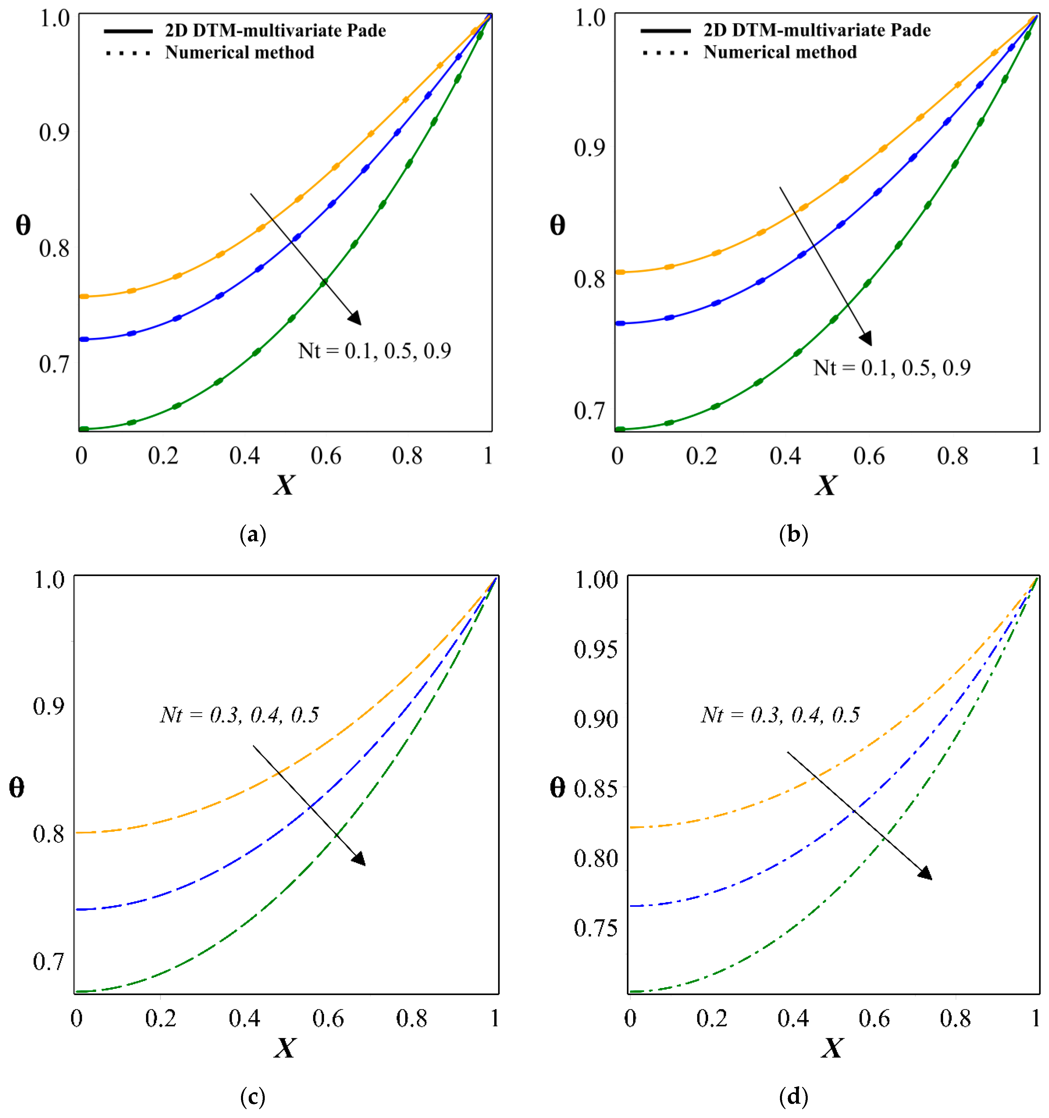
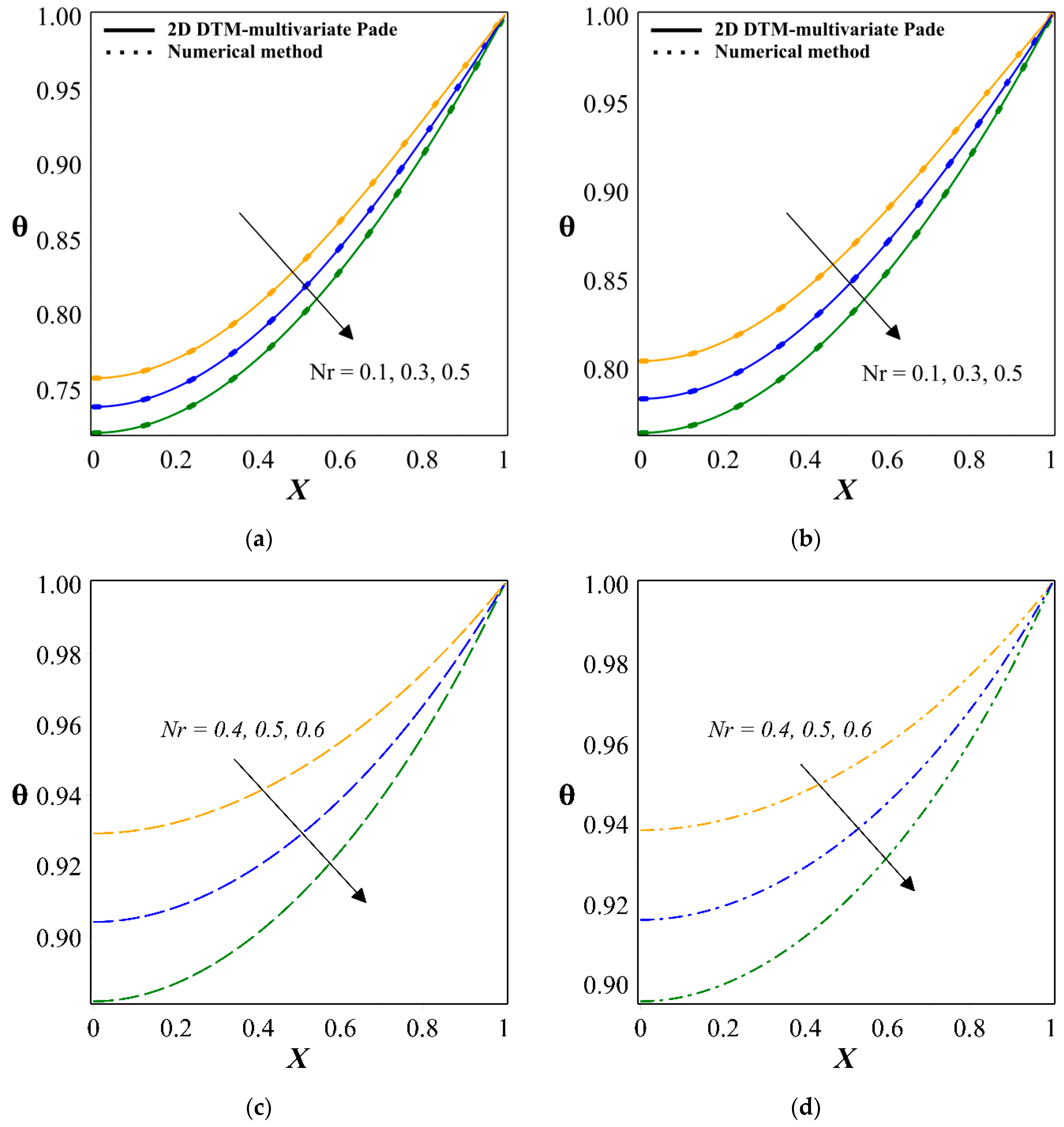
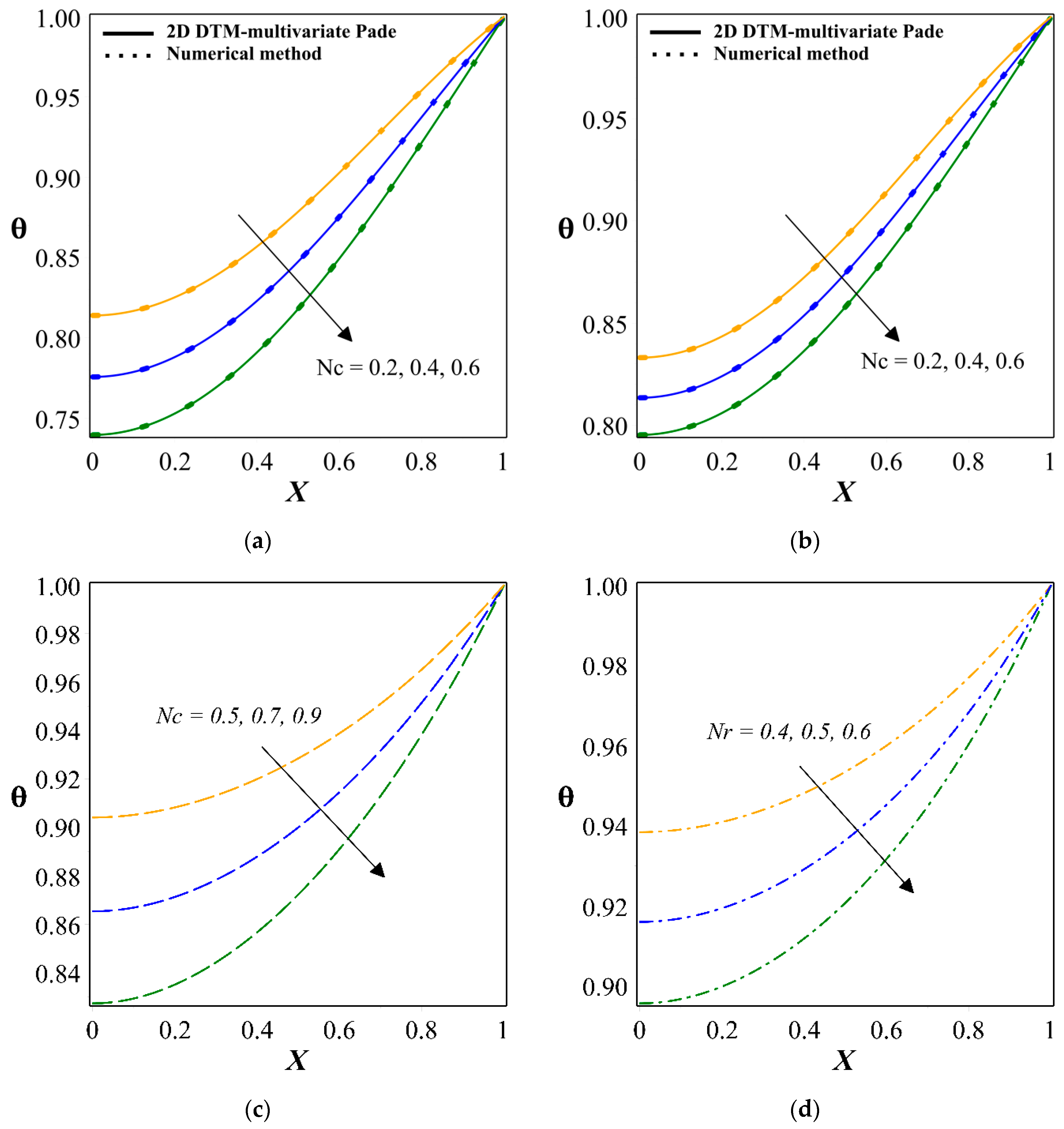
  • An escalation in the magnitude of convection–conduction parameter drops the transient thermal distribution through a moving rod. The same thermal behavior is detected for greater values of temperature ratio parameter and radiation–conduction parameters.
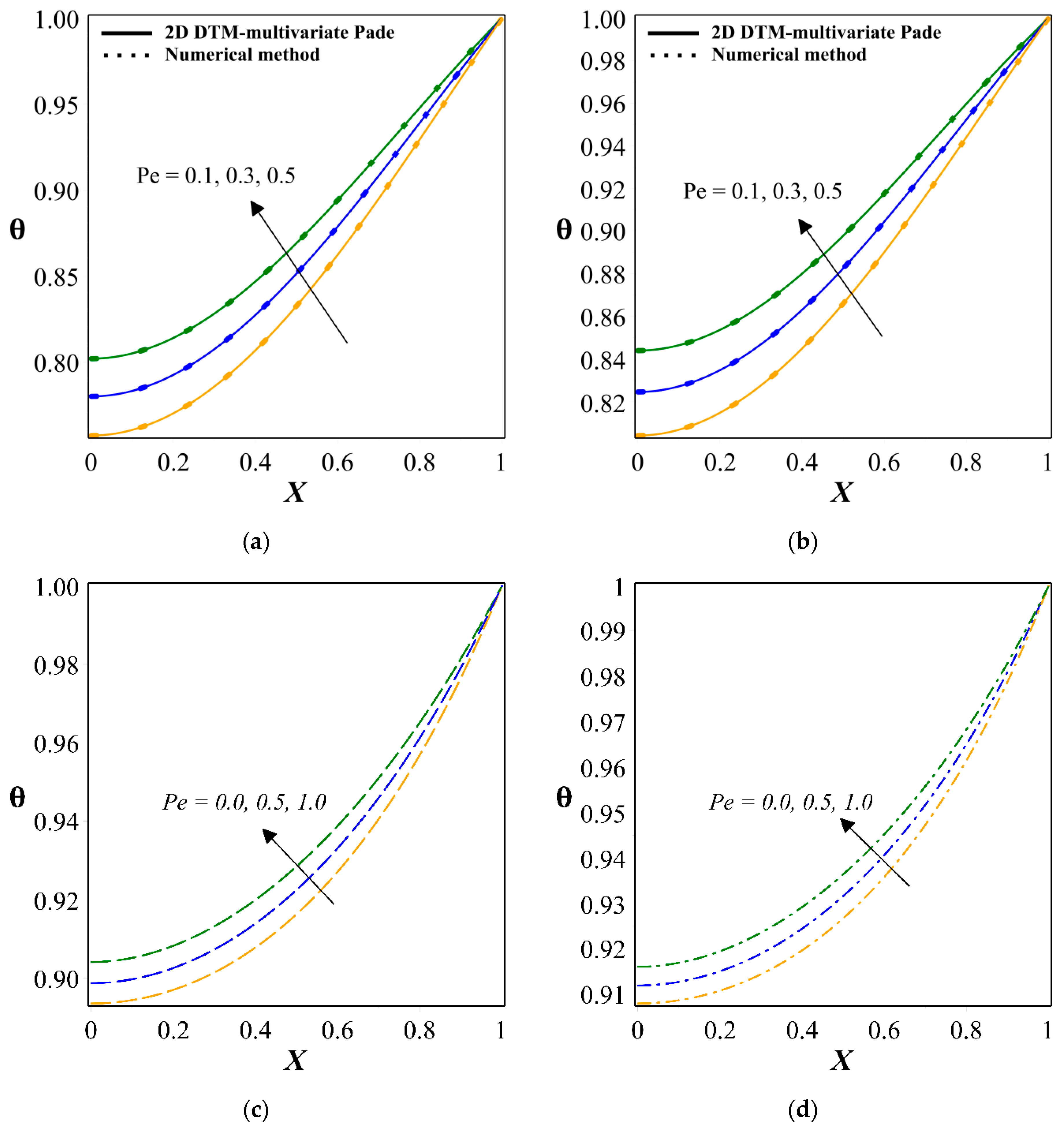
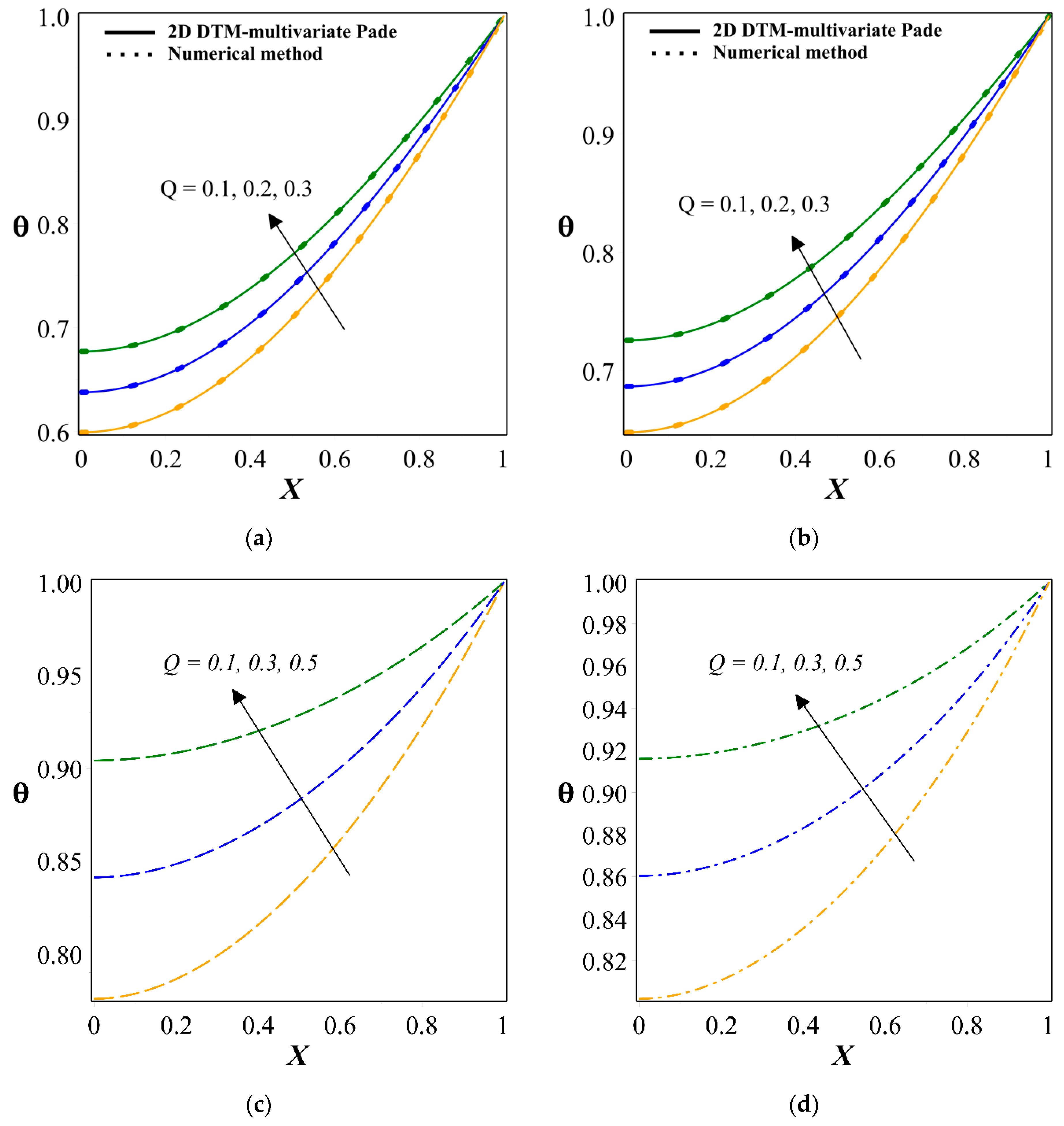
  • A rise in Peclet number increases the transient thermal distribution within the moving rod.
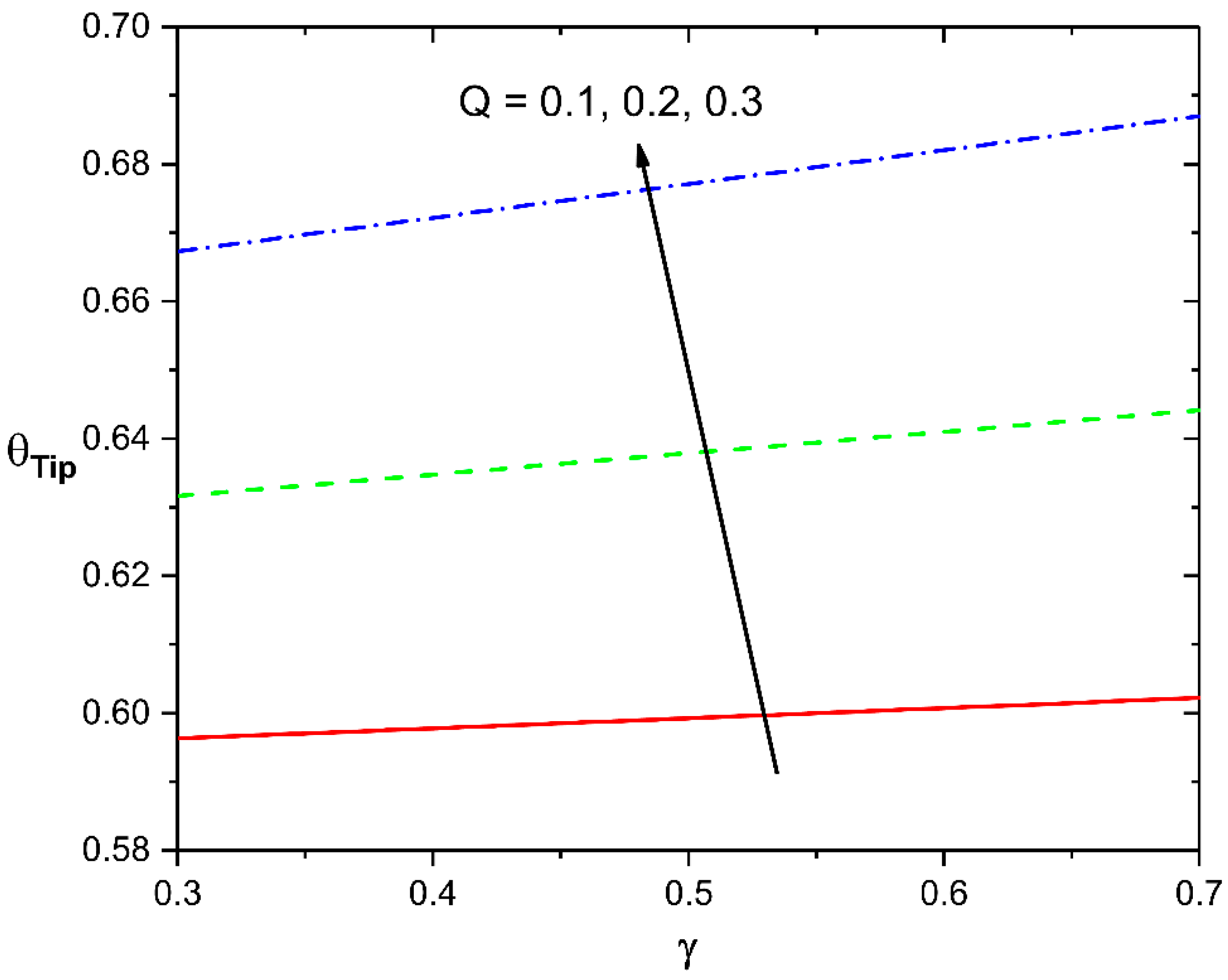
  • The transient thermal distribution enhances with an upsurge in the magnitude of the heat generation parameter.
  • The transient thermal distribution through a rod improves for change in the dimensionless time.
  • The temperature distribution in a moving rod is more for nucleate boiling heat transfer than forced convective heat transfer.
  • Thermal conductivity and heat transfer coefficients are presumed to be temperature-dependent in this inspection. Moreover, the conduction and heat transfer terms are significantly non-linear and represented by power laws. In addition, the various magnitude of physical parameters influences thermal distribution through a moving rod.
  • The tip temperature drops significantly for higher values of the radiative–conductive parameter and the convective–radiative parameter.
  • The aspect of dimensionless temperature profile for the different mechanisms of heat transfer is explained with the graphical explanation. Higher thermal distribution is perceived in the radiative heat transfer process compared to other mechanisms of heat transfer.

Author Contributions

Conceptualization, B.C.P. and I.E.S.; methodology, B.C.P. and I.E.S.; software, G.S. and R.S.V.K.; validation, B.C.P. and I.E.S.; formal analysis, G.S. and R.S.V.K.; investigation, G.S.; resources, I.E.S.; data curation, B.C.P.; writing—original draft preparation, G.S. and R.S.V.K.; writing—review and editing, I.E.S. and B.C.P.; visualization, G.S. and C.S.V.; supervision, B.C.P. and I.E.S.; project administration, I.E.S. All authors have read and agreed to the published version of the manuscript.

Funding

This research received no external funding.

Conflicts of Interest

The authors declare no conflict of interest.

Nomenclature

τ * Dimensionless time ρ Density
T b Constant temperature σ Stefan–Boltzmann constant
L * Dimensionless adjustable length parameter W Width
c p Specific heat capacity P e Peclet number
T a Ambient temperature Q Generation parameter
n Exponent index δ * Thickness
x Coordinate in x-direction ε * Surface emissivity
T Temperature k * Thermal conductivity
τ Time γ Dimensionless heat generation parameter
U Speed of the rod P Perimeter
N t Temperature ratio N c Dimensionless convection–conduction parameter
q * ( T ) Internal heat generation θ Dimensionless temperature
h b Heat transfer coefficient L Dimensionless rod length
N r Dimensionless radiation–conduction parameter X Dimensionless axial coordinate
h * ( T ) Heat transfer coefficient A Cross-sectional area
θ T i p Dimensionless tip temperature m Power index

References

  1. Khan, N.S.; Usman, A.H.; Sohail, A.; Hussanan, A.; Shah, Q.; Ullah, N.; Kumam, P.; Thounthong, P.; Humphries, U.W. A Framework for the Magnetic Dipole Effect on the Thixotropic Nanofluid Flow Past a Continuous Curved Stretched Surface. Crystals 2021, 11, 645. [Google Scholar] [CrossRef]
  2. Tassaddiq, A. Impact of Cattaneo-Christov heat flux model on MHD hybrid nano-micropolar fluid flow and heat transfer with viscous and joule dissipation effects. Sci. Rep. 2021, 11, 1–14. [Google Scholar] [CrossRef]
  3. Kumar, R.S.V.; Dhananjaya, P.G.; Kumar, R.N.; Gowda, R.J.P.; Prasannakumara, B.C. Modeling and theoretical investigation on Casson nanofluid flow over a curved stretching surface with the influence of magnetic field and chemical reaction. Int. J. Comput. Methods Eng. Sci. Mech. 2021, 1–8. [Google Scholar] [CrossRef]
  4. Wahid, N.S.; Arifin, N.M.; Khashi’Ie, N.S.; Pop, I.; Bachok, N.; Hafidzuddin, M.E.H. Flow and heat transfer of hybrid nanofluid induced by an exponentially stretching/shrinking curved surface. Case Stud. Therm. Eng. 2021, 25, 100982. [Google Scholar] [CrossRef]
  5. Yusuf, T.; Mabood, F.; Prasannakumara, B.; Sarris, I. Magneto-Bioconvection Flow of Williamson Nanofluid over an Inclined Plate with Gyrotactic Microorganisms and Entropy Generation. Fluids 2021, 6, 109. [Google Scholar] [CrossRef]
  6. Mabood, F.; Yusuf, T.A.; Khan, W.A. Cu–Al2O3–H2O hybrid nanofluid flow with melting heat transfer, irreversibility analysis and nonlinear thermal radiation. J. Therm. Anal. Calorim. 2021, 143, 973–984. [Google Scholar] [CrossRef]
  7. Dogonchi, A.S.; Ganji, D.D. Convection–radiation heat transfer study of moving fin with temperature-dependent thermal conductivity, heat transfer coefficient and heat generation. Appl. Therm. Eng. 2016, 103, 705–712. [Google Scholar] [CrossRef]
  8. Madhura, K.R.; Babitha; Kalpana, G.; Makinde, O.D. Thermal performance of straight porous fin with variable thermal conductivity under magnetic field and radiation effects. Heat Transf. 2020, 49, 5002–5019. [Google Scholar] [CrossRef]
  9. Sun, S.-W.; Li, X.-F. Exact solution of a non-linear fin problem of temperature-dependent thermal conductivity and heat transfer coefficient. Can. J. Phys. 2020, 98, 700–712. [Google Scholar] [CrossRef]
  10. Das, R.; Kundu, B. Prediction of Heat-Generation and Electromagnetic Parameters from Temperature Response in Porous Fins. J. Thermophys. Heat Transf. 2021, 1–9. [Google Scholar] [CrossRef]
  11. Choudhury, S.R.; Jaluria, Y. Analytical solution for the transient temperature distribution in a moving rod or plate of finite length with surface heat transfer. Int. J. Heat Mass Transf. 1994, 37, 1193–1205. [Google Scholar] [CrossRef]
  12. Aziz, A.; Lopez, R.J. Convection-radiation from a continuously moving, variable thermal conductivity sheet or rod undergoing thermal processing. Int. J. Therm. Sci. 2011, 50, 1523–1531. [Google Scholar] [CrossRef]
  13. Sun, Y.-S.; Ma, J.; Li, B.-W. Spectral collocation method for convective–radiative transfer of a moving rod with variable thermal conductivity. Int. J. Therm. Sci. 2015, 90, 187–196. [Google Scholar] [CrossRef]
  14. Sarwe, D.U.; Shanker, B.; Mishra, R.; Kumar, R.S.V.; Shekar, M.N.R. Simultaneous impact of magnetic and Arrhenius activation energy on the flow of Casson hybrid nanofluid over a vertically moving plate. Int. J. Thermofluid Sci. Technol. 2021, 8. [Google Scholar] [CrossRef]
  15. Onyejekwe, O.O.; Tamiru, G.; Amha, T.; Habtamu, F.; Demiss, Y.; Alemseged, N.; Mengistu, B. Application of an Integral Numerical Technique for a Temperature-Dependent Thermal Conductivity Fin with Internal Heat Generation. J. Eng. Phys. Thermophys. 2020, 93, 1574–1582. [Google Scholar] [CrossRef]
  16. Kezzar, M.; Tabet, I.; Eid, M.R. A new analytical solution of longitudinal fin with variable heat generation and thermal conductivity using DRA. Eur. Phys. J. Plus 2020, 135, 1–15. [Google Scholar] [CrossRef]
  17. Majhi, T.; Kundu, B. New Approach for Determining Fin Performances of an Annular Disc Fin with Internal Heat Generation. In Advances in Mechanical Engineering; Biswal, B., Sarkar, B., Mahanta, P., Eds.; Lecture Notes in Mechanical Engineering; Springer: Singapore, 2020; pp. 1033–1043. [Google Scholar] [CrossRef]
  18. Venkitesh, V.; Mallick, A. Thermal analysis of a convective–conductive–radiative annular porous fin with variable thermal parameters and internal heat generation. J. Therm. Anal. Calorim. 2020, 1–15. [Google Scholar] [CrossRef]
  19. Sowmya, G.; Gireesha, B.J. Thermal stresses and efficiency analysis of a radial porous fin with radiation and variable thermal conductivity and internal heat generation. J. Therm. Anal. Calorim. 2021, 1–12. [Google Scholar] [CrossRef]
  20. Mosayebidorcheh, S.; Ganji, D.D.; Farzinpoor, M. Approximate solution of the nonlinear heat transfer equation of a fin with the power-law temperature-dependent thermal conductivity and heat transfer coefficient. Propuls. Power Res. 2014, 3, 41–47. [Google Scholar] [CrossRef] [Green Version]
  21. Kader, A.H.A.; Latif, M.S.A.; Nour, H.M. General exact solution of the fin problem with the power law temperature-dependent thermal conductivity. Math. Methods Appl. Sci. 2016, 39, 1513–1521. [Google Scholar] [CrossRef]
  22. Ndlovu, P.L.; Moitsheki, R.J. Predicting the Temperature Distribution in Longitudinal Fins of Various Profiles with Power Law Thermal Properties Using the Variational Iteration Method. Defect Diffus. Forum 2018, 387, 403–416. [Google Scholar] [CrossRef]
  23. Zhou, J.K. Differential Transformation and Its Applications for Electrical Circuits; Huazhong University Press: Wuhan, China, 1986. [Google Scholar]
  24. Rashidi, M.M.; Keimanesh, M. Using Differential Transform Method and Padé Approximant for Solving MHD Flow in a Laminar Liquid Film from a Horizontal Stretching Surface. Math. Probl. Eng. 2010, 2010, 1–14. [Google Scholar] [CrossRef]
  25. Domairry, G.; Hatami, M. Squeezing Cu–water nanofluid flow analysis between parallel plates by DTM-Padé Method. J. Mol. Liq. 2014, 193, 37–44. [Google Scholar] [CrossRef]
  26. Sarwe, D.U.; Kulkarni, V.S. Thermal behaviour of annular hyperbolic fin with temperature dependent thermal conductivity by differential transformation method and Pade approximant. Phys. Scr. 2021, 96, 105213. [Google Scholar] [CrossRef]
  27. Turut, V.; Çelik, E.; Yiğider, M. Multivariate padé approximation for solving partial differential equations (PDE). Int. J. Numer. Methods Fluids 2011, 66, 1159–1173. [Google Scholar] [CrossRef]
  28. Turut, V.; Guzel, N.; Zel, N.G. Multivariate Padé Approximation for Solving Nonlinear Partial Differential Equations of Fractional Order. Abstr. Appl. Anal. 2013, 2013, 1–12. [Google Scholar] [CrossRef]
Figure 1. Schematic illustration of a moving rod.
Symmetry 13 01793 g001
Figure 2. (a). Consequence of N t on θ for constant thermal conductivity with n = 0 . (b). Consequence of N t on θ for constant thermal conductivity with n = 2 . (c). Consequence of N t on θ for power-law function of thermal conductivity with n = 0 . (d). Consequence of N t on θ for power-law function of thermal conductivity with n = 2 .
Symmetry 13 01793 g002
Figure 3. (a). Consequence of P e on θ for constant thermal conductivity with n = 0 . (b). Consequence of P e on θ for constant thermal conductivity with n = 2 . (c). Consequence of P e on θ for power-law function of thermal conductivity with n = 0 . (d). Consequence of P e on θ for power-law function of thermal conductivity with n = 2 .
Symmetry 13 01793 g003
Figure 4. (a). Consequence of N r on θ for constant thermal conductivity with n = 0 . (b). Consequence of N r on θ for constant thermal conductivity with n = 2 . (c). Consequence of N r on θ for power-law function of thermal conductivity with n = 0 . (d). Consequence of N r on θ for power-law function of thermal conductivity with n = 2 .
Symmetry 13 01793 g004
Figure 5. (a). Consequence of N c on θ for constant thermal conductivity with n = 0 . (b). Consequence of N c on θ for constant thermal conductivity with n = 2 . (c). Consequence of N c on θ for power-law function of thermal conductivity with n = 0 . (d). Consequence of N c on θ for power-law function of thermal conductivity with n = 2 .
Symmetry 13 01793 g005
Figure 6. (a). Consequence of Q on θ for constant thermal conductivity with n = 0 . (b). Consequence of Q on θ for constant thermal conductivity with n = 2 . (c). Consequence of Q on θ for power-law function of thermal conductivity with n = 0 . (d). Consequence of Q on θ for power-law function of thermal conductivity with n = 2 .
Symmetry 13 01793 g006
Figure 7. (a). Consequence of γ on θ for constant thermal conductivity with n = 0 . (b). Consequence of γ on θ for constant thermal conductivity with n = 2 . (c). Consequence of γ on θ for power-law function of thermal conductivity with n = 0 . (d). Consequence of γ on θ for power-law function of thermal conductivity with n = 2 .
Symmetry 13 01793 g007
Figure 8. (a). Consequence of τ * on θ for constant thermal conductivity with n = 0 . (b). Consequence of τ * on θ for constant thermal conductivity with n = 2 .
Symmetry 13 01793 g008
Figure 9. Consequence of N r on tip temperature θ T i p with respect to N c .
Symmetry 13 01793 g009
Figure 10. Consequence of N t on tip temperature θ T i p with respect to P e .
Symmetry 13 01793 g010
Figure 11. Consequence of Q on tip temperature θ T i p with respect to γ .
Symmetry 13 01793 g011
Figure 12. Nature of θ for various modes of heat transfer.
Symmetry 13 01793 g012
Table 1. The major basic theorems of 2D-DTM considered in this analysis.
Original FunctionTransformed Function
ψ ( y , t ) = α f ( y , t ) + β g ( y , t ) Ψ [ u , v ] = α F ( u , v ) + β G ( u , v ) , where α a n d β are constants
ψ ( y , t ) = y m t n Ψ [ u , v ] = δ ( u m ) δ ( v n ) where δ ( u i ) = { 1           i f u = i , 0          i f u i , and δ ( v j ) = { 1             i f v = j , 0            i f v j ,
ψ ( y , t ) = f ( y , t ) y Ψ [ u , v ] = ( u + 1 ) F ( u + 1 , v )
ψ ( y , t ) = f ( y , t ) t Ψ [ u , v ] = ( v + 1 ) F ( u , v + 1 )
ψ ( y , t ) = f ( y , t ) g ( y , t ) Ψ [ u , v ] = r = 0 u s = 0 v F ( r , v s ) G ( u r , s )
ψ ( y , t ) = f ( y , t ) y g ( y , t ) y Ψ [ u , v ] = r = 0 u ( r + 1 ) F ( r + 1 , v s ) s = 0 v ( u r + 1 ) G ( u r + 1 , s )
ψ ( y , t ) = f ( y , t ) t g ( y , t ) t Ψ [ u , v ] = r = 0 u F ( r + 1 , v s ) s = 0 v ( s + 1 ) G ( u r , s + 1 )
Publisher’s Note: MDPI stays neutral with regard to jurisdictional claims in published maps and institutional affiliations.

