Lagrange Multiplier Test for Spatial Autoregressive Model with Latent Variables

Abstract

The focus of this research is to develop a Lagrange multiplier (LM) test of spatial dependence for the spatial autoregressive model (SAR) with latent variables (LVs). It was arranged by the standard SAR, where the independent variables were replaced by factor scores of the exogenous latent variables from a measurement model (in structural equation modeling) as well as their dependent variables. As a result, an error distribution of the SAR-LVs should have a different distribution from the standard SAR. Therefore, this LM test for the SAR-LVs is based on the new distribution. The estimation of the latent variables used a weighted least squares (WLS) method. The estimation of the SAR-LVs parameter used a two-stage least squares (2SLS) method. The SAR-LVs model was applied to the model with a positive and negative spatial autoregressive coefficient to illustrate how it was interpreted.

1. Introduction

Researchers have often faced models involving latent variables and analyzed the relationships between two or more of those latent variables simultaneously. Latent variables are unobserved or unmeasured variables [1] and measured by connecting to the observed variables because they cannot be directly measured [2]. The statistical methodology that is able to accommodate these two objectives is structural equation modeling (SEM). SEM is a statistical method used to test the relationships between latent variables (path models) and between its observed variables (confirmatory factor models) [2]. In general, SEM has two submodels, namely the measurement model and the structural model. The structural model describes the relationship between latent variables, while the measurement model is the relationship between indicators and the latent variables that construct it.

In social research, analyses involving latent variables and at the same time having a spatial effect have often been found. Spatial dependence may be caused by different kinds of spatial spillover effects. There are two frameworks that involve spatial data in the SEM model, namely at the level of the measurement model or the structural model. The involvement of spatial data at the level of the measurement model is commonly used to analyze multivariate spatial data [3], i.e., when several variables are measured at the same locations over a spatial area, and they are often correlated with each other. Each of them might also be correlated across the locations because of geographic similarities of the different locations.

Christensen and Amemiya [4] suggested a model with a latent variable that is distribution-free to analyze multivariate spatial data. However, it was limited by the assumption of a linear relationship between observed and latent variables that might not apply to Poisson and binomial data. The parameters of the model were estimated by means of a moment method. Wang and Wall [3] proposed the generalized common spatial factor, which was an extension of the traditional factor analysis model. In this model, it was assumed that the common factors were spatially correlated and extended to handle more types of observed data from exponential families, especially Poisson and binomial data.

Hogan and Tchernis [5] proposed the method of a Bayesian hierarchical model for analysis factors of spatially correlated multivariate data. At the first level, the distribution of a vector of manifest variables was conditional on an underlying latent factor in each location, whereas at the second level, the area-specific latent factors had a joint distribution that combined spatial correlation.

In contrast to previous researchers that only analyzed multivariate spatial data in measurement models in the SEM model, Liu et al. [6] developed a generalized spatial structural equation model (GSSEM). They joined the generalized common spatial factor model proposed by Wang and Wall in [3] and SEM that calculated spatial correlations. The GSSEM can also be extended to spatial correlations that can be added to the measurement model. Congdon [7] used the factor analysis on the measurement model. In this model, the construct was observed through indicators. Indicators allowed both spatial correlation and correlation with one another. The relation among constructs that are nonlinear was approached using a spline regression.

Oud and Folmer [8] proposed a SEM approach to the spatial dependence model. They combined the standard spatial model in [9] with the multiple indicators multiple causes (MIMIC) model in [10]. In this approach, the spatial weight that described the spatial spillover effects was located in the structural model. This approach was more flexible and informative compared to modeling that gave the spatial weight to the measurement model. The parameters of this model were estimated using Full Information Maximum Likelihood (FIML) and resulted in an estimator to control the bias of endogeneity due to the interaction between the dependent variable and its lag.

Anekawati et al. [11] conducted modeling of education quality in the senior high school level using the spatial SEM approach. Although they allocated the spatial weight on the structural model, their work had a different perspective on the model in [8]. They developed the spatial SEM model from the standard spatial model by Anselin in [9] but replaced the dependent variables by endogenous latent variables, as well as independent variables. The latent variables were estimated as the factor scores using the partial least squares (PLS) method through iterative estimation developed by Trujillo in [12]. The factor scores were modeled by involving the spatial effects, and the spatial dependence of this model was tested using the Lagrange multiplier (LM) test. The results of the spatial dependence test led to the spatial autoregressive (SAR) model. Furthermore, this model was called the spatial autoregressive model with latent variables (SAR-LVs). The parameters of the SAR-LVs model were estimated using maximum likelihood estimation (MLE).

Anekawati et al. [13] estimated the parameters of the SAR-LVs model from Anekawati et al. in [11] using the generalized method of moment (GMM), which was developed by Kelejian and Prucha in [14,15]. The SAR-LVs model in [13] indicated a better fit for the model than the MLE method since it produced a higher R-square. Additionally, the GMM was computationally easier than MLE.

This idea can be used as alternative modeling involving latent variables and spatial data simultaneously, as the research limitation in [16]. The research purposes in [16] were to identify the relationship between vulnerability factors related to social, economic, and environmental aspects, and economic losses from natural disasters in 230 local communities in South Korea. The social, economic, and environmental aspects were latent variables measured by connecting to the observed variables. The social aspect was constructed by two indicators, namely the percentage of the population over age 15 without elementary school completion and a minority percentage of foreigners. Additionally, the economic and environmental aspects were latent variables. However, the relationship was modeled based on indicators, which were not latent variables. It was less precise to identify the research purpose. That study revealed the limitations of the study, which was an indicator-based approach for the identification of vulnerability factors. Therefore, the method in this study provides an alternative solution for the spatial model that involves latent variables, especially focusing on the spatial dependency test using the LM test.

Oud and Folmer [8] did not perform a diagnostic test of spatial dependence, so there was no direction in determining whether the model led to the spatial autoregressive model or the spatial error model. Anekawati’s research works in [11,13] tested the spatial dependence using the Lagrange multiplier (LM) to diagnose spatial dependence.

One of the constructions of the test of parametric hypotheses based on asymptotic theory is the LM test [17]. Anselin [18] developed the diagnostics for spatial dependence using the LM test. The LM approach seems reasonable and relatively easy based on estimation under the null hypotheses [17], namely, in its most simple form. Yang [19] introduced a residual-based bootstrap method for asymptotically refined approximations to the finite sample critical values of the LM statistics.

The LM test of spatial dependence [18,19] did not involve latent variables for the standard SAR model. Anekawati‘s work [11,13] used the LM test of spatial dependence for the SAR-LVs model, but an error distribution of the model was assumed the same as the standard SAR model in [9,18]. The LM test for the standard SAR model in [9,18] had an assumption that error was normally distributed $\mathsf{\epsilon } \sim N \left(\mathbf{0},{\mathsf{\sigma }}^{2}I\right)$. Meanwhile, the SAR-LVs model was modeled based on the standard SAR model, where factor scores replaced the independent and dependent variables. The factor scores were the estimation result of the latent variables in the submodel in SEM, namely, the measurement model. The measurement model had the assumption that the error was normally distributed, namely, $\mathsf{\delta } \sim N\left(\mathbf{0},{\Theta }_{\mathsf{\delta }}\right)$ for exogenous and ${\mathsf{\epsilon }}^{*}\sim N\left(\mathbf{0},{\Theta }_{{\mathsf{\epsilon }}^{*}}\right)$ for endogenous, while the error distribution in the standard SAR model was $\mathsf{\epsilon } \sim N \left(\mathbf{0},{\mathsf{\sigma }}^{2}I\right)$. As a result, the error distribution of the SAR-LVs model should have a different distribution from the error of the standard SAR model. In this paper, an attempt is made to fill this gap. The focus of this study is to develop a Lagrange multiplier test of spatial dependence for the spatial autoregressive model (SAR) with latent variables (LVs).

To complete this paper, the estimation of latent variables into factor scores uses the weighted least squares (WLS) method, so that the error distribution of the SAR-LVs model is constructed from the result of this estimation. The estimation of parameters of the SAR-LVs model uses the two-stage least squares (2SLS) method. In the last section, the SAR-LVs model is applied for cases of the positive and negative spatial autoregressive coefficient to provide an interpretation of the spatial autoregressive coefficient.

2. Materials and Methods

2.1. Spatial Autoregressive Model with Latent Variable (SAR-LVs Model)

SEM consists of two basic components—the structural model and measurement model in [2]. The measurement model represents the relationship between the manifest variable and exogenous latent variables (1) or endogenous latent variables (2), while the structural model describes the relationship among the latent variables (3). Bollen in [1] wrote the measurement and structural model as Equations (1)–(3).

$$x={\Lambda }_{\mathrm{x} } \mathsf{\xi }+\mathsf{\delta } \mathrm{with} \mathsf{\delta }\sim N_A\left(\mathbf{0},{\Theta }_{\delta }\right)$$

(1)

$$y={\Lambda }_{\mathrm{y} }\mathsf{\eta }+{\mathsf{\epsilon }}^{*} \mathrm{with} {\mathsf{\epsilon }}^{*}\sim N_B\left(\mathbf{0},{\Theta }_{{\mathsf{\epsilon }}^{*}}\right)$$

(2)

$$\mathsf{\eta }=\mathbf{B}\mathsf{\eta }+\mathsf{\Gamma } \mathsf{\xi }+\mathsf{\zeta }$$

(3)

where $\mathsf{\eta }$ is the $\left(q\times 1\right)$ endogenous random vector, $q$ is the number of the endogenous variables, $\mathsf{\xi }$ is the $\left(p\times 1\right)$ exogenous random vector, $p$ is the number of the exogenous variables, $\mathbf{B}$ is the $\left(q\times q\right)$ coefficient matrix that shows the effect of the relationship of an endogenous latent variable to another endogenous variable, $\mathsf{\Gamma }$ is the $\left(q\times p\right)$ coefficient matrix which shows the effect of $\mathsf{\xi }$ relationship to $\mathsf{\eta }$, $\mathsf{\zeta }$ is the $\left(q\times 1\right)$ random error vector, $y$ is the $\left(B\times 1\right)$ observed vector of the endogenous variables, $B$ is a total number of indicators of the endogenous variables, $x$ is the $\left(A\times 1\right)$ observed vector of the exogenous, $A$ is a total number of indicators of the exogenous variables, ${\Lambda }_{\mathrm{y} }$ is the $\left(B\times q\right)$ coefficient matrix which shows the relationship of $y$ to $\mathsf{\eta }$, ${\Lambda }_{\mathrm{x} }$ is the $\left(A\times p\right)$ coefficient matrix which shows the relationship of $x$ to $\mathsf{\xi }$, ${\mathsf{\epsilon }}^{*}$ is the $\left(B\times 1\right)$ measurement error vector of $y$, and $\mathsf{\delta }$ is the $\left(A\times 1\right)$ measurement error vector of $x$.

Assumptions that must be fulfilled are $E\left(\mathsf{\eta }\right)=\mathbf{0}, E\left(\mathsf{\xi }\right)=\mathbf{0}, E\left(\mathsf{\zeta }\right)=\mathbf{0}, E\left(\mathsf{\xi }{\mathsf{\zeta }}^{\prime }\right)=\mathbf{0}, E\left({\mathsf{\epsilon }}^{*}\right)=\mathbf{0}, E\left(\mathsf{\delta }\right)=\mathbf{0}, \left(\mathbf{I}-\mathbf{B}\right)$ is nonsingular, and the element of error vectors of measurements, namely ${\delta }_i$ and ${\mathsf{\epsilon }}_i^{*} ,$ are homoscedastic and nonautocorrelated across observations (see [1]).

Anselin wrote the standard SAR model in [9]:

$$y^{*}=\lambda W{y}^{*}+X\mathsf{\beta }+\mathsf{\epsilon } \mathrm{with} \mathsf{\epsilon } \sim N \left(\mathbf{0},{\mathsf{\sigma }}^{2}I\right),$$

(4)

where $y^{*}$ is the $\left(T\times 1\right)$ spatially lagged dependent vector, $T$ is the number of the observed units, $X$ is the $\left(T\times \left(p+1\right)\right)$ exogenous matrix, $\lambda$ is coefficient of $y^{*}$, $\mathsf{\beta }$ is the $\left(\left(p+1\right)\times 1\right)$ parameters vector of exogenous, $W$ is the $\left(T\times T\right)$ spatial weight matrix with the main diagonal elements being zero, $\mathsf{\epsilon }$ is the $\left(T\times 1\right)$ disturbance vector, where it is the classic homoscedastic situation. The queen contiguity method was used for spatial weighting. In queen contiguity, W_ij is defined as 1 for the entity where the common side or the common vertex meets the region of concern, and W_ij is defined as 0 for other regions [20].

Oud and Folmer in [8] wrote the SAR-LVs model in the form of the MIMIC. The proposed model was $\tilde{\mathsf{\eta }}=\lambda W\tilde{\mathsf{\eta }}+\tilde{X}\gamma +\tilde{\mathsf{\zeta }}$, where $\lambda$ was the spatial lag coefficient of the endogenous variable, $W$ was the contiguity matrix, and $\tilde{X}$ was the observation matrix of the explanatory variable.

The SAR-LVs model is a model that involves latent variables, and the unit of observation is location. The SAR-LVs model is a standard SAR model in which the independent and dependent variables are latent variables. In the SEM model, there are latent variables that cannot be measured directly as a sample unit. Therefore, in this work, to represent the latent variable in the standard SAR in Equation (4) is changed by the factor score. The latent variable is replaced by the factor score from the measurement model in Equations (2) and (3) as a measured and random unit sample. As seen in Equation (4), the spatially lagged dependent variable $\left(y^{*}\right)$ is changed by the endogenous latent variable ($\mathsf{\eta }$), and the exogenous variable ($X$) is changed by the exogenous latent variable ($\mathsf{\xi }$), which is previously estimated using the WLS method. The result of estimation of the latent variable is denoted by $\widehat{\mathsf{\eta }}=\mathit{l}$ and $\widehat{\mathsf{\xi }}=\mathbf{K}$. This SAR-LVs model does not use the MIMIC model, since there are no exogenous or endogenous variables that are observed variables, and the endogenous variable is limited to only one.

Thus, the SAR-LVs model in Equation (4) changes to:

$$\mathit{l}=K\mathsf{\beta }+\lambda W\mathit{l}+\mathsf{\epsilon } ,$$

(5)

where $\mathit{l}$ is the the $\left(T\times 1\right)$ endogenous factor score vector, $\mathbf{K}$ is the $\left(T\times \left(p+1\right)\right)$ exogenous factor score matrix, and $\mathsf{\beta }$ is the $\left(\left(p+1\right)\times 1\right)$ regression coefficient vector.

2.2. Estimation of Score of Latent Variable

The factor score is the estimation result of the latent variables, both the endogenous and exogenous variables in the measurement model. The method used is the WLS, which is by minimizing the sum squared errors that are weighted by the error variant matrix. In the estimation process, to obtain a factor score, it is assumed that the value of the loading factor and the error variant matrix are constant.

In the equation of the measurement model of the exogenous latent variable (1), where $p$ is the number of the exogenous latent variable, $a_i$ is the number of indicators of the ith exogenous latent variable, and ${\displaystyle \sum }_{i=1}^p{a}_i=A. \mathsf{\delta }$ is an error, where $\mathsf{\delta }\sim N_A\left(\mathbf{0},{\Theta }_{\delta }\right)$ with ${\Theta }_{\delta }\left(A\times A\right)$ is the covariant–variant matrix of measurement error of observed variable $\mathit{x}$, namely

$${\Theta }_{\delta }=diag\left({\sigma }_{{\delta }_{\left(1\right)1}}^2,{\sigma }_{{\delta }_{\left(2\right)1}}^2,\cdots ,{\sigma }_{{\delta }_{\left(a1\right)1}}^2,{\sigma }_{{\delta }_{\left(a1\right)2}}^2,{\sigma }_{{\delta }_{\left(a2\right)2}}^2,\cdots ,{\sigma }_{{\delta }_{\left(a2\right)2}}^2,\cdots ,{\sigma }_{{\delta }_{\left(1\right)p}}^2,{\sigma }_{{\delta }_{\left(2\right)p}}^2,\cdots ,{\sigma }_{{\delta }_{\left(ap\right)p}}^2\right).$$

The distribution of $x$ is obtained through the properties of the expected value and variance of a random variable. It is assumed that the value of ${\Lambda }_{\mathrm{x}}$ and ${\Theta }_{\delta }$ are constant. $E\left(x\right)=E\left({\Lambda }_{\mathrm{x}} \mathsf{\xi }+\mathsf{\delta }\right)={\Lambda }_{\mathrm{x}} \mathsf{\xi }$ and $var\left(x\right)=var\left({\Lambda }_{\mathrm{x}} \mathsf{\xi }+\mathsf{\delta }\right)=var\left(\mathsf{\delta }\right)={\Theta }_{\delta }$. Therefore, if $x={\Lambda }_{\mathrm{x}} \mathsf{\xi }+\mathsf{\delta }$ and $\mathsf{\delta } \sim N_A\left(\mathbf{0},{\Theta }_{\delta }\right)$ then the distribution of $x$ is $x \sim N_A\left({\Lambda }_{\mathrm{x}}\mathsf{\xi },{\Theta }_{\delta }\right)$. Suppose that a random sample T is given from a random variable $x$

$$\left(x_{\left(x\right)11},x_{\left(2\right)12},\cdots ,x_{\left(a_i\right)1T},x_{\left(1\right)21},x_{\left(2\right)22},\cdots ,x_{\left(a_2\right)2T},\cdots ,x_{\left(1\right)p\mathit{l}},x_{\left(2\right)pT},x_{\left(a_p\right)pT,{\mathsf{\xi }}_{11},{\mathsf{\xi }}_{12},\cdots ,{\mathsf{\xi }}_{1T}{}_{,}{\mathsf{\xi }}_{21},{\mathsf{\xi }}_{22},\dots ,{\mathsf{\xi }}_{2T},\dots ,{\mathsf{\xi }}_{p1},{\mathsf{\xi }}_{p2},\dots {\mathsf{\xi }}_{pT}}\right)$$

with t = 1, 2, …, T so $x_t \sim N_A\left({\Lambda }_{\mathrm{x}}{\mathsf{\xi }}_t,{\Theta }_{\delta }\right)$. The probability function of $x_t$ is

$$f\left(X_t\right)={(2\pi )}^{-\frac{A}{2}}{\left|{\Theta }_{\delta }\right|}^{-\frac{1}{2}} exp\left\{-\frac{1}{2}{\left(x_t-{\Lambda }_{\mathrm{x}}{\mathsf{\xi }}_t\right)}^{\prime }{\Theta }_{\delta }^{-1}\left(x_t-{\Lambda }_{\mathrm{x}}{\mathsf{\xi }}_t\right)\right\}$$

The likelihood function is

$$L\left(\mathsf{\xi },{\Theta }_{\delta }\right)=(2{\pi )}^{-\frac{AT}{2}}{\left|{\Theta }_{\delta }\right|}^{-\frac{T}{2}} exp\left\{-\frac{1}{2}{Q}_x\right\} \mathrm{with} Q_x={\sum }_{t=1}^T{\left(x_t-{\Lambda }_{\mathrm{x}}{\mathsf{\xi }}_t\right)}^{\prime }{\Theta }_{\delta }^{-1}\left(x_t-{\Lambda }_{\mathrm{x}}{\mathsf{\xi }}_t\right)$$

The latent variable $\mathsf{\xi }$ is estimated using the WLS method with optimization $L(\mathsf{\xi },{\Theta }_{\delta }$). Maximum $L \left(\mathsf{\xi },{\Theta }_{\delta }\right)⟺\min Q_x$ by adding the weight of an error variant matrix ${\Theta }_{\delta }$ is obtained as ${\displaystyle \sum }_{t=1}^T{\widehat{\mathsf{\xi }}}_t=\left({\Lambda }_{\mathrm{x}}^{\prime }{\Theta }_{\delta }^{-1}{\Lambda }_{\mathrm{x}}\right)\left({\Lambda }_{\mathrm{x}}^{\prime }{\Theta }_{\delta }^{-1}\right){\displaystyle \sum }_{t=1}^T{x}_t$ or can be written in matrix form and contain each element as

$$\left(\begin{array}{cccc}{ \hat{\mathsf{\xi }}}_{11}& { \hat{\mathsf{\xi }}}_{12}& \cdots & { \hat{\mathsf{\xi }}}_{1T}\\ { \hat{\mathsf{\xi }}}_{21}& { \hat{\mathsf{\xi }}}_{22}& \cdots & { \hat{\mathsf{\xi }}}_{2T}\\ ⋮& ⋮& \ddots & ⋮\\ { \hat{\mathsf{\xi }}}_{p1}& { \hat{\mathsf{\xi }}}_{p2}& \cdots & { \hat{\mathsf{\xi }}}_{pT}\end{array}\right)=\left({\Lambda }_{\mathrm{x}}^{\prime }{\Theta }_{\delta }^{-1}{\Lambda }_{\mathrm{x}}\right)\left({\Lambda }_{\mathrm{x}}^{\prime }{\Theta }_{\delta }^{-1}\right)\left(\begin{array}{cccc}{\mathrm{x}}_{\left(1\right)11}& {\mathrm{x}}_{\left(1\right)12}& \cdots & {\mathrm{x}}_{\left(1\right)1T}\\ {\mathrm{x}}_{\left(2\right)11}& {\mathrm{x}}_{\left(2\right)12}& \cdots & {\mathrm{x}}_{\left(2\right)1T}\\ ⋮& ⋮& \ddots & ⋮\\ {\mathrm{x}}_{\left(a_1\right)11}& {\mathrm{x}}_{\left(a_1\right)12}& \cdots & {\mathrm{x}}_{\left(a_1\right)1T}\\ {\mathrm{x}}_{\left(1\right)21}& {\mathrm{x}}_{\left(1\right)22}& \cdots & {\mathrm{x}}_{\left(1\right)2T}\\ {\mathrm{x}}_{\left(2\right)21}& {\mathrm{x}}_{\left(2\right)22}& \cdots & {\mathrm{x}}_{\left(2\right)2T}\\ ⋮& ⋮& \ddots & ⋮\\ {\mathrm{x}}_{\left(a_2\right)21}& {\mathrm{x}}_{\left(a_2\right)22}& \cdots & {\mathrm{x}}_{\left(a_2\right)22}\\ ⋮& ⋮& \ddots & ⋮\\ {\mathrm{x}}_{\left(1\right)p1}& {\mathrm{x}}_{\left(1\right)p2}& \cdots & {\mathrm{x}}_{\left(1\right)pT}\\ {\mathrm{x}}_{\left(2\right)p1}& {\mathrm{x}}_{\left(2\right)p2}& \cdots & {\mathrm{x}}_{\left(2\right)p2}\\ ⋮& ⋮& \ddots & ⋮\\ {\mathrm{x}}_{\left(a_p\right)p1}& {\mathrm{x}}_{\left(a_p\right)p2}& \cdots & {\mathrm{x}}_{\left(a_p\right)pT}\end{array}\right)$$

By assuming matrix $\left(\begin{array}{cccc}{ \hat{\mathsf{\xi }}}_{11}& { \hat{\mathsf{\xi }}}_{12}& \cdots & { \hat{\mathsf{\xi }}}_{1T}\\ { \hat{\mathsf{\xi }}}_{21}& { \hat{\mathsf{\xi }}}_{22}& \cdots & { \hat{\mathsf{\xi }}}_{2T}\\ ⋮& ⋮& \ddots & ⋮\\ { \hat{\mathsf{\xi }}}_{p1}& { \hat{\mathsf{\xi }}}_{p2}& \cdots & { \hat{\mathsf{\xi }}}_{pT}\end{array}\right)={\mathbf{K}}^{\prime }$ and $X=\left(\begin{array}{cccc}{\mathrm{x}}_{\left(1\right)11}& {\mathrm{x}}_{\left(1\right)12}& \cdots & {\mathrm{x}}_{\left(1\right)1T}\\ {\mathrm{x}}_{\left(2\right)11}& {\mathrm{x}}_{\left(2\right)12}& \cdots & {\mathrm{x}}_{\left(2\right)1T}\\ ⋮& ⋮& \ddots & ⋮\\ {\mathrm{x}}_{\left(a_1\right)11}& {\mathrm{x}}_{\left(a_1\right)12}& \cdots & {\mathrm{x}}_{\left(a_1\right)1T}\\ {\mathrm{x}}_{\left(1\right)21}& {\mathrm{x}}_{\left(1\right)22}& \cdots & {\mathrm{x}}_{\left(1\right)2T}\\ {\mathrm{x}}_{\left(2\right)21}& {\mathrm{x}}_{\left(2\right)22}& \cdots & {\mathrm{x}}_{\left(2\right)2T}\\ ⋮& ⋮& \ddots & ⋮\\ {\mathrm{x}}_{\left(a_2\right)21}& {\mathrm{x}}_{\left(a_2\right)22}& \cdots & {\mathrm{x}}_{\left(a_2\right)22}\\ ⋮& ⋮& \ddots & ⋮\\ {\mathrm{x}}_{\left(1\right)p1}& {\mathrm{x}}_{\left(1\right)p2}& \cdots & {\mathrm{x}}_{\left(1\right)pT}\\ {\mathrm{x}}_{\left(2\right)p1}& {\mathrm{x}}_{\left(2\right)p2}& \cdots & {\mathrm{x}}_{\left(2\right)p2}\\ ⋮& ⋮& \ddots & ⋮\\ {\mathrm{x}}_{\left(a_p\right)p1}& {\mathrm{x}}_{\left(a_p\right)p2}& \cdots & {\mathrm{x}}_{\left(a_p\right)pT}\end{array}\right)$, so

$$K^{\prime }=\left({\Lambda }_{\mathrm{x}}^{\prime }{\Theta }_{\delta }^{-1}{\Lambda }_{\mathrm{x}}\right)\left({\Lambda }_{\mathrm{x}}^{\prime }{\Theta }_{\delta }^{-1}\right)X.$$

(6)

$X$ in Equation (6) is a random observation matrix. Based on Definition A.1 in [21] (Appendix A), $X$ has normal distribution $X \sim N_{A,T }\left({\Lambda }_{\mathrm{x}}{\mathsf{\xi }}_t{e}^{\prime },{\Theta }_{\delta }⨂I_T\right)$, where ${\mathit{e}}_{T\times 1}=\left(1,\dots ,1\right)$.

The definition of the characteristic function of the random matrix $X$ is ${\varphi }_x\left(Z\right)=E \left[etr \left(\iota X{Z}^{\prime }\right)\right]$, where $\iota =\sqrt{-1}$. If part of Equation (6) is assumed $\left({\Lambda }_{\mathrm{x}}^{\prime }{\Theta }_{\delta }^{-1}{\Lambda }_{\mathrm{x}}\right)\left({\Lambda }_{\mathrm{x}}^{\prime }{\Theta }_{\delta }^{-1}\right)=P$ then Equation (6) can be simplified into $K^{\prime }=XP$. The characteristic function of $K^{\prime }$ is ${\varphi }_{K^{\prime }}\left(Z\right)=E \left[etr\left(\iota \left(PX\right)Z^{\prime }\right)\right]=E \left[etr \left(\iota P\left(X{Z}^{\prime }\right)\right)\right]$. Based on Theorem B.1, the characteristic function of $K^{\prime }$ can be changed into ${\varphi }_{K^{\prime }}\left(Z\right)=E \left[etr\left(\iota X\left(Z^{\prime }P\right)\right)\right]$. If $Z_1^{\prime }=Z^{\prime }P$ then the characteristic function of $K^{\prime }$ can be changed into ${\varphi }_{K^{\prime }}\left(Z\right)=E\left[etr (\iota X{Z}_1^{\prime }\right]$.

The distribution of X is $X\sim N_{A,T }\left({\Lambda }_{\mathrm{x}}{\mathsf{\xi }}_t{e}^{\prime },{\Theta }_{\delta }⨂I_T\right)$ and $K^{\prime }=XP$. Based on Theorem A.2, the characteristic function of $K^{\prime }$ is ${\varphi }_{K^{\prime }}\left(Z\right)=etr \left(\iota Z_1^{\prime }{\Lambda }_{\mathrm{x}}{\mathsf{\xi }}_t{e}^{\prime }-1/2Z_1^{\prime }{\Theta }_{\delta }{Z}_1{I}_T\right)$. If $Z_1^{\prime }$ is changed by $Z_1^{\prime }=Z^{\prime }P$ then the characteristic function of $K^{\prime }$ is ${\varphi }_{K^{\prime }}\left(Z\right)=etr \left(\iota \left(Z^{\prime }P\right){\Lambda }_{\mathrm{x}}{\mathsf{\xi }}_t{e}^{\prime }-1/2{\left(Z^{\prime }P\right)}^{\prime }{\Theta }_{\delta }\left(Z^{\prime }P\right)I_T\right)$ Furthermore, $P$ is changed by $P=\left({\Lambda }_{\mathrm{x}}^{\prime }{\Theta }_{\delta }^{-1}{\Lambda }_{\mathrm{x}}\right)\left({\Lambda }_{\mathrm{x}}^{\prime }{\Theta }_{\delta }^{-1}\right)$, so the characteristic function of $K^{\prime }$ is

$${\varphi }_{K^{\prime }}\left(Z\right)=etr \left(\iota Z^{\prime }{\mathsf{\xi }}_t{e}^{\prime }-1/2Z^{\prime }{\left({\Lambda }_{\mathrm{x}}^{\prime }{\Theta }_{\delta }^{-1}{\Lambda }_{\mathrm{x}}\right)}^{-1}Z{I}_T\right)$$

(7)

Based on Theorem A.2 and Equation (7), $K^{\prime }$ is the matrix variate normal distribution with mean ${\mathsf{\xi }}_t{e}^{\prime }$ and covariate matrix ${\left({\Lambda }_{\mathrm{x}}^{\prime }{\Theta }_{\delta }^{-1}{\Lambda }_{\mathrm{x}}\right)}^{-1}⨂I_T$ and is notated by $K^{\prime } \sim N_{T, p }\left({\mathsf{\xi }}_t{e}^{\prime },{\left({\Lambda }_{\mathrm{x}}^{\prime }{\Theta }_{\delta }^{-1}{\Lambda }_{\mathrm{x}}\right)}^{-1}⨂I_T\right)$. Based on Theorem A.1, $K$ is the matrix variate normal distribution that is notated by:

$$K\sim N_{T, p }\left(e{\mathsf{\xi }}_t,I_T⨂{\left({\Lambda }_{\mathrm{x}}^{\prime }{\Theta }_{\delta }^{-1}{\Lambda }_{\mathrm{x}}\right)}^{-1}\right).$$

(8)

In this paper, the number of the endogenous variables is limited only to one. The covariance matrix of the measurement error of the observed variable for $y$ is ${\Theta }_{{\epsilon }^{*}}$, namely ${\Theta }_{{\epsilon }^{*}}=diag \left({\sigma }_{{\epsilon }_1^{*}}^2,{\sigma }_{{\epsilon }_2^{*}}^2,\dots ,{\sigma }_{{\epsilon }_B^{*}}^2\right)$, where $B$ is the number of indicators of the endogenous latent variable. In the same way as the previous estimation with the exogenous latent variable and by assuming that vector $\left({\hat{\mathsf{\eta }}}_{1 }{\hat{\mathsf{\eta }}}_{2 }\dots {\hat{\mathsf{\eta }}}_{t }\right)={\mathit{l}}^{\prime }$ and $Y=\left(\begin{array}{ccc}\begin{array}{c}{y}_{11}\\ y_{21}\\ \begin{array}{c}⋮\\ y_{B1}\end{array}\end{array}& \begin{array}{c}{y}_{12}\\ y_{22}\\ \begin{array}{c}⋮\\ y_{B2}\end{array}\end{array}& \begin{array}{cc}\begin{array}{c}\cdots \\ \cdots \\ \begin{array}{c}\ddots \\ \cdots \end{array}\end{array}& \begin{array}{c}{y}_{1T}\\ y_{2T}\\ \begin{array}{c}⋮\\ y_{BT}\end{array}\end{array}\end{array}\end{array}\right)$, it is obtained

$${\mathit{l}}^{\prime }={\left({\Lambda }_y^{\prime } {\Theta }_{\epsilon *}^{-1} {\Lambda }_y\right)}^{-1} {\Lambda }_y^{\prime } {\Theta }_{\epsilon *}^{-1} Y,$$

(9)

and its distribution is

$$\mathit{l}\sim N_T \left(e{\mathsf{\eta }}_t,{\left({\Lambda }_y^{\prime } {\Theta }_{\epsilon *}^{-1} {\Lambda }_y\right)}^{-1}{\mathbf{I}}_T\right).$$

(10)

Theorem A.1, A.2, and B.1 are provided in Appendix A.

2.3. The Error Distribution of The SAR-LVs Model

The equation of the SAR-LVs model from the estimated factor score can be arranged as Equation (6) and adding ${\mathsf{\beta }}_0,$ it can be written as

$$\mathit{l}=K \mathsf{\beta }+\lambda W\mathit{l} +\mathsf{\epsilon },$$

(11)

or can be written in the matrix form

$$\left(\begin{array}{c}{l}_1\\ l_2\\ ⋮\\ l_T\end{array}\right)=\left(\begin{array}{ccccc}1& {\mathrm{k}}_{11}& {\mathrm{k}}_{12}& \cdots & {\mathrm{k}}_{1p}\\ 1& {\mathrm{k}}_{21}& {\mathrm{k}}_{22}& \cdots & {\mathrm{k}}_{2p}\\ ⋮& ⋮& ⋮& \ddots & ⋮\\ 1& {\mathrm{k}}_{T1}& {\mathrm{k}}_{T2}& \cdots & {\mathrm{k}}_{Tp}\end{array}\right)\left(\begin{array}{c}{\mathsf{\beta }}_0\\ {\mathsf{\beta }}_1\\ {\mathsf{\beta }}_2\\ ⋮\\ {\mathsf{\beta }}_p\end{array}\right)\left(\begin{array}{c}{l}_1\\ l_2\\ ⋮\\ l_T\end{array}\right)+\left(\begin{array}{c}{\mathsf{\epsilon }}_1\\ {\mathsf{\epsilon }}_2\\ ⋮\\ {\mathsf{\epsilon }}_T\end{array}\right)$$

where $K\sim N_{T, p }\left(e{\mathsf{\xi }}_t,I_T⨂{\left({\Lambda }_{\mathrm{x}}^{\prime }{\Theta }_{\delta }^{-1}{\Lambda }_{\mathrm{x}}\right)}^{-1}\right)$ is Equation (6) and $\mathit{l}\sim N_T \left(e{\mathsf{\eta }}_t,{\left({\Lambda }_y^{\prime } {\Theta }_{\epsilon *}^{-1} {\Lambda }_y\right)}^{-1}{\mathbf{I}}_T\right)$ is Equation (10).

The SAR-LVs model (11) is a spatial regression model by considering $\mathit{l}$ as a response variable and $K$ as a predictor variable, both of which are random. Thus, the function of $\mathit{l}$ is $f\left(\mathit{l}|K\right)$, so that the variable $K$ is no longer random but fixed. As a result, the error in Equation (11) is $\mathsf{\epsilon }=\left(\mathbf{I}-\lambda W\right)\mathit{l}-K\mathsf{\beta }$ where $\mathit{l}$ is a random variable, $K$ is fixed and is assumed not to correlate with $\mathsf{\epsilon }$, and $cov\left(\mathit{l},K\right)\ne \mathbf{0}$.

The expectation value of $\mathsf{\epsilon }$ is $E \left(\mathsf{\epsilon }\right)=\left(\mathbf{I}-\lambda W\right)e{\mathsf{\eta }}_t- K\mathsf{\beta }$, and the variance of $\mathsf{\epsilon }$ is $var\left(\mathsf{\epsilon }\right)=\left(\mathbf{I}-\lambda W\right) {\left({\Lambda }_y^{\prime } {\Theta }_{\mathsf{\epsilon }*}^{-1} {\Lambda }_y\right)}^{-1}{\left(\mathbf{I}-\lambda W\right)}^{\prime }$, so the error distribution of $\mathsf{\epsilon }$ is

$$\mathsf{\epsilon } \sim N_T \left(\left(\mathbf{I}-\lambda W\right)e{\mathsf{\eta }}_t- K\mathsf{\beta },\Theta \right),$$

(12)

where

$$\Theta =\left(\mathbf{I}-\lambda W\right) {\left({\Lambda }_y^{\prime } {\Theta }_{\mathsf{\epsilon }*}^{-1} {\Lambda }_y\right)}^{-1}{\left(\mathbf{I}-\lambda W\right)}^{\prime }.$$

(13)

The error distribution of the standard SAR model is $\mathsf{\epsilon }\sim N \left(\mathbf{0},{\sigma }^{2}I\right)$, while the error distribution of the SAR-LVs model is as Equation (12). This error distribution is used to construct the LM test.

2.4. Test of Dependency Spatial

The Lagrange multiplier (LM) test of the SAR-LVs model, as shown in Equation (11), is a test based on estimation under the null hypothesis. The likelihood function $\mathrm{l}$ in the SAR-LVs model is obtained by replacing $\mathsf{\epsilon }$ and multiplying by the Jacobian in the Gaussian function so that the likelihood function for the SAR-LVs model is obtained: $\mathrm{L}\left(\lambda ,\mathsf{\beta },\Theta ;\mathit{l}\right)={\mathsf{\pi }}^{-\mathrm{T}/2}|{\Theta |}^{-1/2}|C|\exp \left(-\frac{1}{2}{\mathsf{\epsilon }}^{\prime }{\Theta }^{-1}\mathsf{\epsilon }\right)$, where $C=\left(\mathbf{I}-\lambda W\right)$.

The log-likelihood function for the SAR-LVs model is $ℒ\left(\lambda ,\mathsf{\beta },\Theta ;\mathit{l}\right)=-\frac{\mathrm{T}}{2}\ln \left|\mathsf{\pi }\right|-\frac{1}{2}\ln \left|\Theta \right|+\ln \left|C\right|-\frac{1}{2}\left({\mathsf{\epsilon }}^{\prime }{\Theta }^{-1}\mathsf{\epsilon }\right)$, where the value of $\Theta$ is as in Equation (13), and $\mathsf{\epsilon }=\left(\mathbf{I}-\lambda W\right)\mathit{l}-\mathbf{K}\mathsf{\beta }$.

Breusch and Pagan in [17] defined LM test statistics as follows: ${\mathrm{LM}}_{\lambda }={\widehat{D}}_{\lambda }^{\prime }{\widehat{\mathsf{\Psi }}}_{\lambda \lambda }^{-1}{\widehat{D}}_{\lambda }$, where ${\widehat{\mathsf{\Psi }}}_{\lambda \lambda }^{-1}$ is an element of an information matrix measuring $\mathrm{k}\times \mathrm{k}$ whose elements are the second derivative of each parameter estimated as ${\widehat{\mathsf{\psi }}}_{\mathsf{\theta }}=\mathrm{E}\left[-\frac{{\partial }^2ℒ\left(\mathsf{\theta }\right)}{\partial \mathsf{\theta }\partial {\mathsf{\theta }}^{\prime }}\right]$. The test was under the null hypothesis, so ${\widehat{D}}_{\lambda }$ is the first derivative of the log-likelihood function of $\lambda$ where $\lambda =\mathbf{0}$.

The value of ${\widehat{\mathsf{\Psi }}}_{\lambda \lambda }^{-1}$ and ${\widehat{D}}_{\lambda }$ were decomposed in Appendix A, which obtained ${ \tilde{\mathsf{\Psi }}}_{\lambda \lambda }^{-1}=-{\mathrm{p}}^{-1}{\left({\left(e{\mathsf{\eta }}_t- K\mathsf{\beta }\right)}^{\prime }W{W}^{\prime }\left(e{\mathsf{\eta }}_t- K\mathsf{\beta }\right)\right)}^{-1}$ so ${\widehat{D}}_{\lambda }=\mathrm{p}{\left(WK\mathsf{\beta }\right)}^{\prime }\left(\mathit{l}-K \mathsf{\beta }\right)$ where $\left(\mathit{l}-\mathbf{K}\mathsf{\beta }\right)$ is an error of the OLS regression model, $\mathit{l}-\mathbf{K}\mathsf{\beta }=\tilde{\mathsf{\epsilon }}$, so ${\widehat{D}}_{\lambda }=\mathrm{p}{\left(WK\mathsf{\beta }\right)}^{\prime }\tilde{\mathsf{\epsilon }}$. The LM statistic test is

$$L{M}_{\lambda }=\frac{-{\left(\mathrm{p}{\left(WK\mathsf{\beta }\right)}^{\prime }\tilde{\mathsf{\epsilon }}\right)}^2}{\mathrm{p}{\left(e{\mathsf{\eta }}_t- K\mathsf{\beta }\right)}^{\prime }W{W}^{\prime }\left(e{\mathsf{\eta }}_t- K\mathsf{\beta }\right)}$$

where $\mathrm{p}=\left({\Lambda }_y^{\prime } {\Theta }_{\epsilon *}^{-1} {\Lambda }_y\right)$ and $\mathrm{d}={\left(e{\mathsf{\eta }}_t- K\mathsf{\beta }\right)}^{\prime }W{W}^{\prime }\left(e{\mathsf{\eta }}_t- K\mathsf{\beta }\right)$, so the value of test statistic LM becomes

$$L{M}_{\lambda }=\frac{-{\left(\mathrm{p}{\left(WK\mathsf{\beta }\right)}^{\prime }\tilde{\mathsf{\epsilon }}\right)}^2}{\mathrm{pd}}$$

(14)

The LM statistics $L{M}_{\lambda }$ follows the asymptotic distribution of ${\chi }_{\left(1\right)}^2$.

2.5. Estimation of Parameter of SAR-LVs Model

If the parameter of the SAR-LVs model in Equation (11) and its error distribution as Equation (12) are estimated by the OLS, then the estimator is biased and inconsistent, since there is a case where the regression variable $\left(W\mathit{l}\right)$ correlates with the error ε or $cov\left(W\mathit{l},\mathsf{\epsilon }\right) \ne \mathbf{0}$. If the model is estimated by the moment method, the overidentified condition is obtained. The following explains the overidentified condition.

The Equation (11) can be simplified as follows:

$$\mathit{l}=Z\alpha +\mathsf{\epsilon },$$

(15)

where $Z$ is $Z=\left(K|W\mathit{l}\right)$ and has the $\left(T\times \left(p+2\right)\right)$-sized, $\mathsf{\alpha }$ is $\mathsf{\alpha }={\left({\mathsf{\beta }}^{\prime }|\lambda \right)}^{\prime }$ and has the the $\left(\left(\mathrm{p}+2\right)\times 1\right)$-sized.

In this work, δ as Equation (15) was estimated by the 2SLS method as performed by [14,15], namely two steps of the ordinary least squares (OLS) method as follows: (i). The 2SLS method requires an $H$ instrument variable, which is a joint of the $K$ matrix and the $WK$ matrix or written as $H=\left(K|WK\right)$. The instrument variable $H$ is valid because it does not correlate with $\mathsf{\epsilon }$ and correlates with regressor $W\mathit{l}$; (ii). Regress $W\mathit{l}$ on instrument variable $H$ to obtain $\widehat{W\mathit{l}}=H{\left(H^{\prime }H\right)}^{-1}{H}^{\prime }\left(W\mathit{l}\right)$; (iii). Regress $\mathit{l}$ on $\widehat{Z}$ to obtain

$$\widehat{\alpha }={(\widehat{Z^{\prime }}\widehat{Z})}^{-1}{\widehat{Z}}^{\prime }\mathit{l},$$

(16)

where $\widehat{Z}=\left(K|\widehat{W\mathit{l}}\right)$ and $\widehat{\mathsf{\alpha }}$ which contains $\widehat{\mathsf{\beta }}$ and $\hat{\lambda }$.

3. Results and Discussion

In the discussion, this study examined two cases or models developed with the results of positive and negative spatial autoregressive coefficient to provide an interpretation of the spatial autoregressive coefficient. The first case was the education quality model developed by [13], with updated data in 2018 and showing a negative spatial autoregressive coefficient. Meanwhile, the second case related to a poverty model conducted by [22] producing a positive spatial autoregressive coefficient.

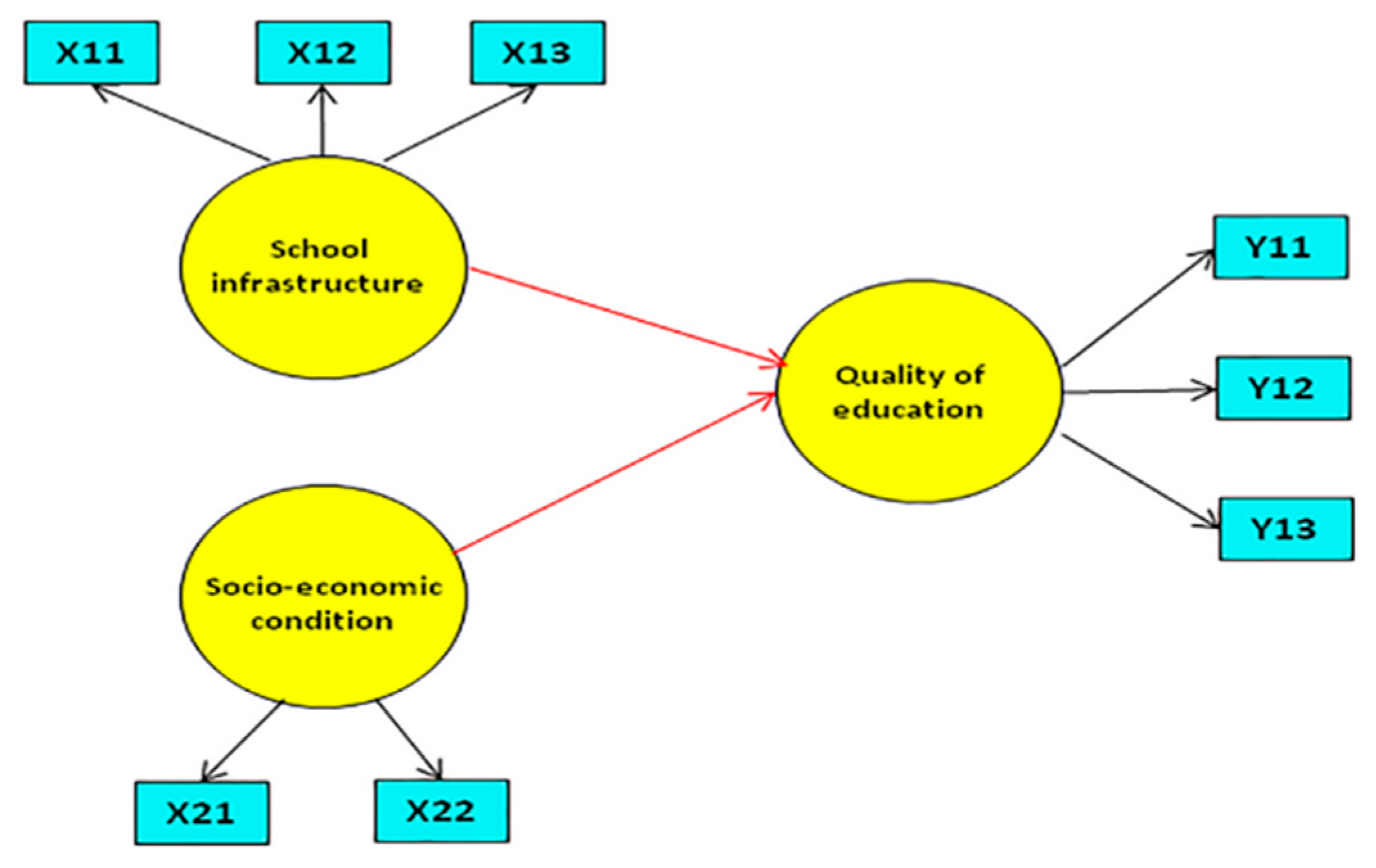
The education quality model for senior high schools in Sumenep Regency involved 27 observation units, one endogenous latent variable, and two exogenous latent variables. The endogenous latent variable was the education quality with three indicators. Indicators of education quality were the ratio of the gross enrolled number of senior high school students to the number of children aged between 15 and 18 years in each district (Y11)—the ratio of the number of accredited senior high schools with at least B levels to the total number of senior high schools in each district (Y12) and the average of national exam scores of senior high school students in each district (Y13).

Exogenous latent variables were school infrastructure and socioeconomic conditions. Indicators of school infrastructure were the proportion of the number of schools with a minimum classroom space according to the regulations of the national education ministry (X11), the proportion of the numbers of schools with laboratories according to the regulations of the national education ministry (X12), and the proportion of the number of schools with libraries according to the regulations of the national education ministry (X13).

Indicators of socioeconomic conditions were the ratio of the number of households running a home industry or with a shop at home to the total number of households in each district (X21) and the ratio of the number of households using clean water to the total number of households in each district (X22). The model is shown in Figure 1.

Latent variables were estimated as in the Equations (6) and (9), then were modeled as in the Equation (11). The estimation of the model parameters as the Equation (16) used the Matlab software, and the results are shown in

Table 1. The estimation result of parameter and spatial autoregressive coefficient for the education model.

Variable	Coefficient
School Infrastructure (b1)	2.3121
Socioeconomic condition (b2)	0.1286
Constant (b0)	9.6604
Spatial Autoregressive Coefficient (λ)	−0.002

. The LM test based on the Equation (14) used Matlab software, and the obtained value ${\mathrm{LM}}_{\lambda }$ was −2.3272. The value of ${\mathrm{LM}}_{\lambda }$ was compared to ${\chi }^2$ with degrees of freedom of one and $\alpha =5\%$. Then, the result was significant towards the SAR-LVs model. Additionally, the spatial autoregressive coefficient was negative.

In general, the SAR-LVs model for the education quality of the senior high school is: $l_i=9.6604-0.002{\displaystyle \sum }_{\mathrm{j}=1,\mathrm{i}\ne \mathrm{j}}^{27}{\mathrm{W}}_{\mathrm{ij}}{l}_j+2.3121{\mathrm{k}}_1+0.1286{\mathrm{k}}_2$, where $l_i$ is the education quality in the i-th district, ${\mathrm{k}}_1$ is the infrastructure, and ${\mathrm{k}}_2$ is socioeconomic condition.

The spatial dependence test result was significant. This means there was a correlation between the education quality of the senior high schools in one district and the one in other contiguous districts. The negative spatial autoregressive coefficient interpreted the opposite of the common spillover effect, i.e., a district was supported by or gained a spillover effect of the neighboring districts’ education quality.

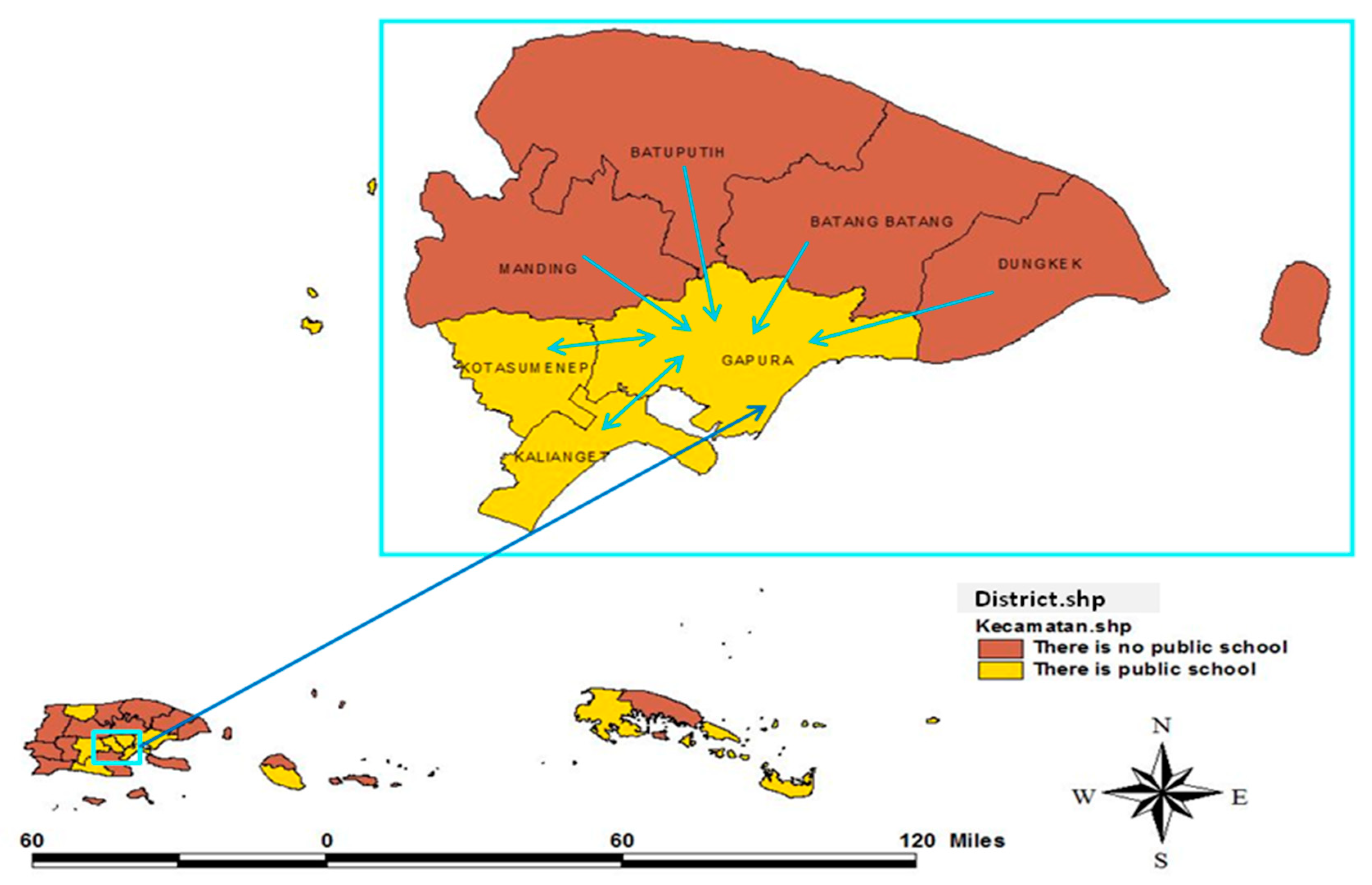
The spillover effect of the neighboring districts’ education quality was generally due to the migration of students to find high-quality schools in the neighboring districts. As a result, the districts that had high-quality schools, gained the spillover effect of quality education through high-achieving students from the neighboring districts. In general, high-quality schools in Sumenep Regency are public schools. Figure 2 draws the distribution of districts with and without public schools. To illustrate the student migration, an example is provided in the Gapura district (see Figure 2).

Table 2. Number of students and public schools for the neighboring of Gapura district.

District	Number of Public Senior High Schools	Number of Junior High School Graduate Students	Number of New Senior High School Students
Kalianget	1	488	744
Kota Sumenep	3	1582	2041
Manding	0	201	93
Batuputih	0	226	143
Gapura	1	485	622
Batang Batang	0	552	360
Dungkek	0	409	156

shows the number of junior high school graduates and new senior high school students for seven districts in the same year, 2018, based on [23]. This table provides an overview of the migration data of students entering senior high school among districts. The Gapura District was used as an example to illustrate student migration (see Figure 2 and Table 2). The Gapura District has one public school and six neighboring neighbors (queen contiguity). Based on Table 2, the Gapura District has 485 junior high school graduates and 622 new high school students. This means that there was a migration of students to the Gapura District.

The Gapura District received the spillover effect of quality education from neighboring districts, especially those with no public schools. The quality spillover was due to schools in the Gapura district having the opportunity to select the best students from the district itself or the neighboring districts.

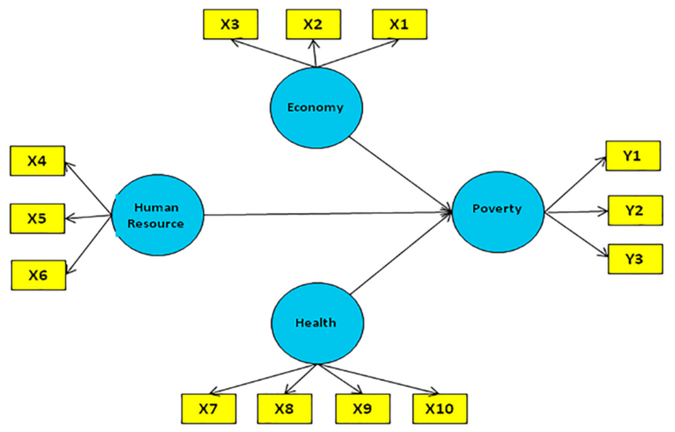
The second case was the poverty model in East Java province, with an observation unit of 38 regencies. This model had one endogenous latent variable, namely poverty, and three exogenous latent variables, namely Economy, Human Resource, and Health. Poverty indicators were the percentage of the poor population (Y1), the index of poverty depth (Y2), and the index of poverty severity (Y3). Indicators of economics were the percentage of poor people around 15 years old or more who were unemployed (X1), the percentage of poor people aged 15 years old or more who were working in agriculture (X2), and the percentage of households gaining Raskin (X3). Raskin is an Indonesian subsidy program to provide rice for people who live under the poverty line. Indicators of Human Resources were the percentage of poor people aged 15 years old and over who did not complete elementary education (X4), the literacy rate of the poor aged from 15 to 55 years (X5), and the participation rates in schools for the poor aged from 13 to 15 years (X6). Health indicators were the percentage of women using KB (Family planning program) devices in poor households (X7), the percentage of children under five in poorly immunized households (X8), the percentage of poor households using drinking water (X9), and the percentage of poor households using private/together latrines (X10). The model is shown in Figure 3.

Latent variables were estimated as in the Equations (6) and (9), then were modeled as in the Equation (11). The estimation of the model parameters as in the Equation (16) used the Matlab software, and the results are shown in

Table 3. The estimation result of parameter and spatial autoregressive coefficient for the poverty model.

Variable	Coefficient
Economy (b1)	0.0742
Human Resource (b2)	−0.0722
Health (b3)	0.0155
Constant (b0)	7.0881
Spatial Autoregressive Coefficient (λ)	0.2345

. The LM test based on Equation (14) used the Matlab software, and the obtained value ${\mathrm{LM}}_{\lambda }$ was −4965. The value of ${\mathrm{LM}}_{\lambda }$ was compared to ${\chi }^2$ with degrees of freedom of one and $\alpha =5\%$. Then, the result was significant towards the SAR-LVs model. Meanwhile, the spatial autoregressive coefficient was positive.

In general, the SAR-LVs model for the poverty is $l_i=7.0881+0.2345{\displaystyle \sum }_{\mathrm{j}=1,\mathrm{i}\ne \mathrm{j}}^{38}{\mathrm{W}}_{\mathrm{ij}}{l}_j+0.0742{\mathrm{k}}_1-0.0722{\mathrm{k}}_2+0.0155{\mathrm{k}}_3$, where $l_i$ is poverty in the i-th regency, ${\mathrm{k}}_1$ is Economy, ${\mathrm{k}}_2$ is Human Resource, and ${\mathrm{k}}_3$ is Health.

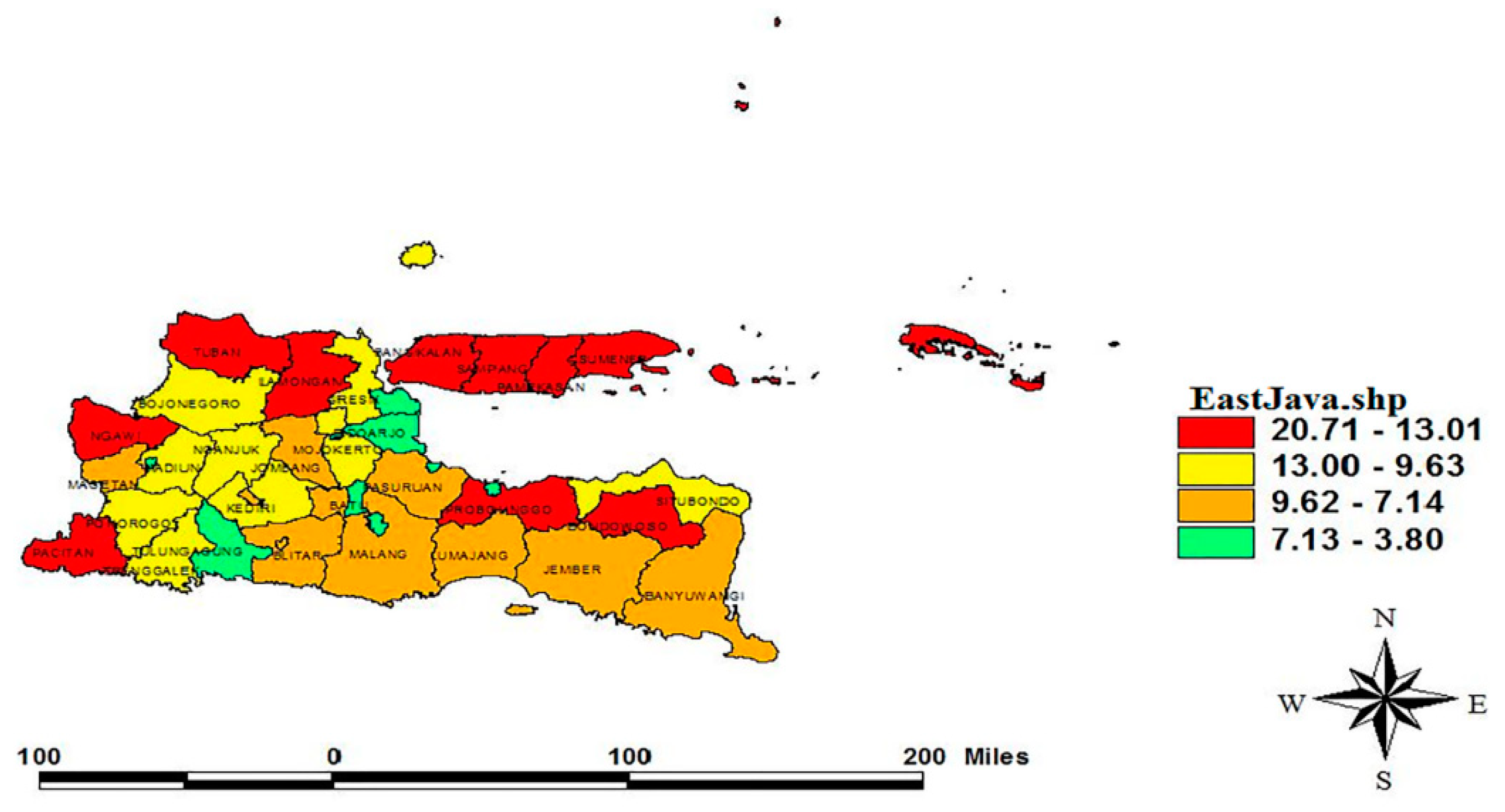
The spatial dependence test result was significant. This means there was a correlation between poverty in one regency and the one in other contiguous regencies. The positive spatial autoregressive coefficient interpreted the common spillover effect, i.e., a regency gives a poverty spillover effect to the neighboring regencies. Figure 4 describes the poor people distribution in the East Java province measured in percent. The percentage of poor people was based on the poverty data in [24] and was clustered into four quartiles. The regency with the high percentage of poor people was categorized as the first quartile (red zone), with 20.71–13.01%. On the other hand, the fourth quartile (green zone) includes the regency with 7.13–3.80% of the poor group. The first quartile was the regency group with the highest percentage of poor people, and so on until the fourth quartile was the regency group with the lowest percentage of poor people. According to Figure 4, the location of regencies in the first quartile was always close to the regencies in the first and the second quartile. This visualization reinforces the results of the multiplier Lagrange test that there is a spatial effect where one regency gives the influence of poverty on its neighboring regencies.

The finding of this method provides value for policymakers relating to existing problems. The first case was the negative spatial autoregressive coefficient for the education quality model. It interpreted that a district was supported by or gained a spillover effect of the neighboring districts’ education quality through students’ migration. This case needs the policy to strive for quality standardization for all schools. The second case was the positive spatial autoregressive coefficient for the poverty model. It interpreted that a regency gives a poverty spillover effect to the neighboring regencies. Policymakers need this information to assist at the locus of poverty appropriately.

4. Conclusions

The SAR-LVs model is a standard SAR model in which the independent and dependent variables are latent variables. The standard SAR model is $y^{*}=\lambda W{y}^{*}+X\mathsf{\beta }+\mathsf{\epsilon }$. The variable of $y^{*}$ is changed by the endogenous factor score ($\widehat{\mathsf{\eta }}$), and $X$ is changed by the exogenous factor score ($\widehat{\mathsf{\xi }}$). The estimation of the latent variables uses the WLS method and assumes that the value of ${\Lambda }_{\mathrm{x}}$ and ${\Theta }_{\delta }$ are constant. Therefore, the SAR-LVs model can be modeled as $\mathit{l}=K \mathsf{\beta }+\lambda W\mathit{l} +\mathsf{\epsilon }$, where $\widehat{\mathsf{\eta }}=\mathit{l}$ and $\widehat{\mathsf{\xi }}=\mathbf{K}$. The distribution of $\mathbf{K}$ and $\mathit{l}$ are $K\sim N_{T, p }\left(e{\mathsf{\xi }}_t,I_T⨂{\left({\Lambda }_{\mathrm{x}}^{\prime }{\Theta }_{\delta }^{-1}{\Lambda }_{\mathrm{x}}\right)}^{-1}\right)$ and $\mathit{l}\sim N_T \left(e{\mathsf{\eta }}_t,{\left({\Lambda }_y^{\prime } {\Theta }_{\epsilon *}^{-1} {\Lambda }_y\right)}^{-1}{\mathbf{I}}_T\right)$. The variables of $\mathit{l}$ and $K$ are random. Thus, the function of $\mathit{l}$ is $f\left(\mathit{l} |K\right)$, so that the variable $K$ is no longer random but fixed. The error distribution is obtained through the properties of the expected value and the variance of the error in the SAR-LVs model, namely $\mathsf{\epsilon }\sim N_T \left(\left(\mathbf{I}-\lambda W\right)e{\mathsf{\eta }}_t- K\mathsf{\beta },\Theta \right),$ where $\Theta =\left(\mathbf{I}-\lambda W\right) {\left({\Lambda }_y^{\prime } {\Theta }_{\epsilon *}^{-1} {\Lambda }_y\right)}^{-1}{\left(\mathbf{I}-\lambda W\right)}^{\prime }$. Based on its error distribution model, so under the null hypothesis, the LM statistic is $L{M}_{\lambda }=\frac{-{\left(\mathrm{p}{\left(WK\mathsf{\beta }\right)}^{\prime }\tilde{\mathsf{\epsilon }}\right)}^2}{\mathrm{pd}}$ and follows the asymptotic distribution of ${\mathrm{X}}_{\left(1\right)}^2$.

Some significant limitations of this study need to be considered. Firstly, the number of endogenous latent variables is one. Future studies can be developed for the higher number of endogenous latent variables. Secondly, the LM test developed was merely for SAR-LVs. Future studies can be developed for a spatial error model with latent variables (SEM-LVs).