Multifractal Analysis of Movement Behavior in Association Football

Abstract

Research in football has been embracing the complex systems paradigm in order to identify different insights about key determinants of performance. The present study explored the multifractal properties of several football-related scenarios, as a candidate method to describe movement dynamics. The sample consisted of five footballers that were engaged in six different training situations (jogging, high intensity interval protocol, running circuit, 5 vs. 5, 8 vs. 8 and a 10 vs. 10 small-sided game). All kinematic measures were collected using a 100 Hz wireless and wearable inertial measurement unit (WIMUPRO©). Data were processed using a discrete wavelet leader transform in order to obtain a spectrum of singularities that could best describe the movement dynamics. The Holder exponent for each of all six conditions revealed mean values h < 0.5 indicating presence of long memory with anti-correlated behavior. A strong trend was found between the width of the multifractal spectrum and the type of task performed, with jogging showing the weakest multifractality ∆h = 0.215 ± 0.020, whereas, 10 vs. 10 small-sided game revealed the strongest ∆h = 0.992 ± 0.104. The Hausdorff dimension indicates that a maximal fluctuation rate occurs with a higher probability than that of the minimal fluctuation rate for all tasks, with the exception of the high intensity interval protocol. Moreover, the spectrum asymmetry values of jogging, running circuit, 5 vs. 5, 8 vs. 8 and 10 vs. 10 small-sided games reveal their multifractal structures are more sensitive to the local fluctuations with small magnitudes. The multifractal analysis has shown a potential to systematically elucidate the dynamics and variability structure over time for the training situations.

1. Introduction

Wearable technologies have widened the scope and the research questions about the key determinants of sport performance [1,2]. For example, technological development has provided the advent of new tracking devices and training-monitoring systems that allow sports scientists to explore interactions between tactical dimensions and physiological aspects of elite performance in team sports [3,4]. Furthermore, high-frequency inertial measurement units (IMUs) are being used to capture the players’ locomotion and, thus, providing a valid measure to assist in the understanding of movement dynamics [5,6]. As an example, several studies have described the use of accelerometers to detect physical activities, movement patterns and to identify activity profiles in team sports players [5,7,8].

The way that each player moves on the pitch obeys the team’s collective dynamics, thus depicting great variability of behavior with different magnitudes and temporal dynamics [9]. According to Sampaio and Maçãs [10], such behavior features highly nonlinear, deterministic and stochastic characteristics, furthermore, the measurement of complex biological systems such as human locomotion via IMUs, often generates extremely irregular signals that tend to exhibit intricate characteristics such as nonlinearity, extreme variations, nonstationarity and fluctuations on a wide range of time scales [11,12,13,14]. In such a scenario, expertise in signal processing techniques is becoming mandatory, in order to overcome issues with analyses and fully explore the information contained in these signals.

Although the human movement is characterized as a complex system, the current mathematical and statistical approaches to analyze the movement of football players are mostly based on deterministic-nonspecific tools (i.e., discretization). An important limitation of the discretization process is due to the fact that a sequence of a continuous variable is represented only by a finite number of data points. Hence, in doing so, a huge amount of data containing important information about the dynamical behavior of the signal of interest is lost [15,16]. A secondary limitation that emerges from the discretization process that has, in practice, a considerable impact, is the large difference between the algorithms used for the discretization procedure that yield coefficient of variations as large as 10–43% for acceleration and 42–56% for deceleration efforts during a team sport simulation protocol [15]. In addition, the adoption of arbitrarily chosen thresholds to depict the magnitude of acceleration zones (i.e., low, moderate and high) are, at least, nonconsensual. Thus, considering the above-mentioned issues, there seems to be a limitation in understanding the dynamical behavior of football players.

Several methodological frameworks have been developed to provide numerical evidence for the study of complexity in signal analysis. Fractal theory stands out as one of the most important theories that has been developed with this purpose [11]. The concepts of fractals and scaling have enlightened the analysis of complex signals during the last decade. According to Stergiou and Decker [14] mathematical tools such as fractal measures have enabled the evaluation of the temporal structure of the variability of human movement behavior. In a recent work by Barbosa et al. [17], fractal measures exhibited the complexity properties of swimming technique. The authors found the lowest values of fractal dimension and speed fluctuation in front-crawl and backstroke, followed by butterfly and breaststroke.

Fractals generally characterize a rough or fragmented geometry that can be recursively split into parts, that can be viewed approximately or as stochastically reduced-size copies of the whole [18]. The fractals appear infinitely complex and irregular when an object is zoomed in and shows self-similarity at all levels of magnification. These characteristics can be observed in nature (e.g., snowflakes, clouds, mountain ranges or coastlines) and in biology (e.g., a bronchial tree or cardiovascular system). Thus, fractals are ubiquitous in nature and its concepts have spanned through geometry, mathematics, statistics and signal processing.

Accordingly, applying the concept of fractals to the analysis of complex signals means that the performance of a given descriptive statistical measure “μ” (i.e., sum, mean, variance, etc.) depends on the corresponding scale of observation in a power–law fashion. The global scale exponent α describes how the statistical descriptor behaves across scales, and is defined by the following power–law relation of the scale-dependent measure of μ_s:

$${\mu }_s \propto s^{\alpha } s \to 0$$

(1)

The global scale exponents α are calculated as the slope of the linear regression between the log (μ_s) versus the log (s). It follows that, if the slope of the log–log plot between the scale of observation and the descriptive statistics is equal 0 < α < 0.5, then the process has a memory, and it exhibits anti-correlations. Therefore, the successive random elements in a sequence present an increasing trend in the past that is likely to be followed by a decreasing trend in the future, and vice-versa. Conversely, if the slope is equal to 0.5 < α < 1, then the process has a memory, and it exhibits positive correlations. Therefore, the successive random elements in a sequence present an increasing trend in the past that is likely to be followed by an increasing trend in the future. If the slope is α = 0.5, then the process is indistinguishable from a random process with no memory (random walk). Finally, if the slope is 1 < α < 2, then the process is non-stationary. Most real-world phenomena yield signals that mix different patterns of correlations over time and in different time scales, most often presenting irregular behavior with interwoven periods of high and low correlation. In such cases the linear regression of log₂μ(s) on log₂s does not exhibit a straight-line characterizing mono-scaling behavior by a single scale exponent, conversely, additional exponents are necessary. In fact, signals with interwoven fractal subsets become more complex, hence requiring multiple scaling exponents for the full description of different parts of the signal. Consequently, in contrast to the monofractal formalism, where a global scale exponent α is defined for the entire signal, multifractal time series are defined by a set of local singularity exponents. According to Ihlen and Vereijken [19], signals present in biological systems exhibit multiscaling behavior, for example, signals of inter-stride intervals in human walking or inter-beat interval in electrocardiogram data. Moreover, almost all data points in the aforementioned signals can be represented as a singularity at time instant t₀ with a strength that is numerically defined by a singularity exponent α. These apparent random variations can be misinterpreted as pure noise originating from the system, however, studying the correlation structure of noise-like signals can elucidate important information about the process underpinning its generation.

Summing up all the previous considerations, there is a clear opportunity to explore how the multifractal analysis can reveal new insights about sports performance and discuss how its outcomes can extend current knowledge in the particular topic of movement analysis in football. Therefore, the aim of this study is to identify the multifractal spectrum of different football-related activities (jogging, high intensity interval protocol, circuit running, 5 vs. 5, 8 vs. 8 and 10 vs. 10 small-sided games).

2. Materials and Methods

2.1. Participants

Five young football players (16.6 ± 0.5 years, 1.76 ± 0.03 m height, and 68.4 ± 4.2 kg body mass) participated in this study. Criteria for inclusion were applied to ensure all players were engaged in amateur competitions and organized training schedules for, at least, 3 times a week. They also would have to be injury-free for at least 3 months. Participants, their legal guardians and their coaching staff, were fully informed about the purpose, benefits and risks of the study, and were provided with written informed consent before the study started. The study protocol conformed to the recommendations of the Declaration of Helsinki and was approved by the local institution (UID/DTP/04045/2019).

2.2. Data Collection

Inertial data of all participants were collected using individual WIMU units (RealTrack Systems, Almería, Spain). The validity and reliability of WIMU© system have been already reported previously and their operation procedures and handling are well documented elsewhere [20]. In order to decrease the measurement errors, the players used the same unit across all the testing situations. Accelerometer data were sampled at 100 Hz. After each session, data were downloaded using proprietary software (WIMU PRO, Real Track System, Almeria, Spain) and raw data were carried for further analysis with MATLAB^® software (MathWorks, Inc., Natick, MA, USA).

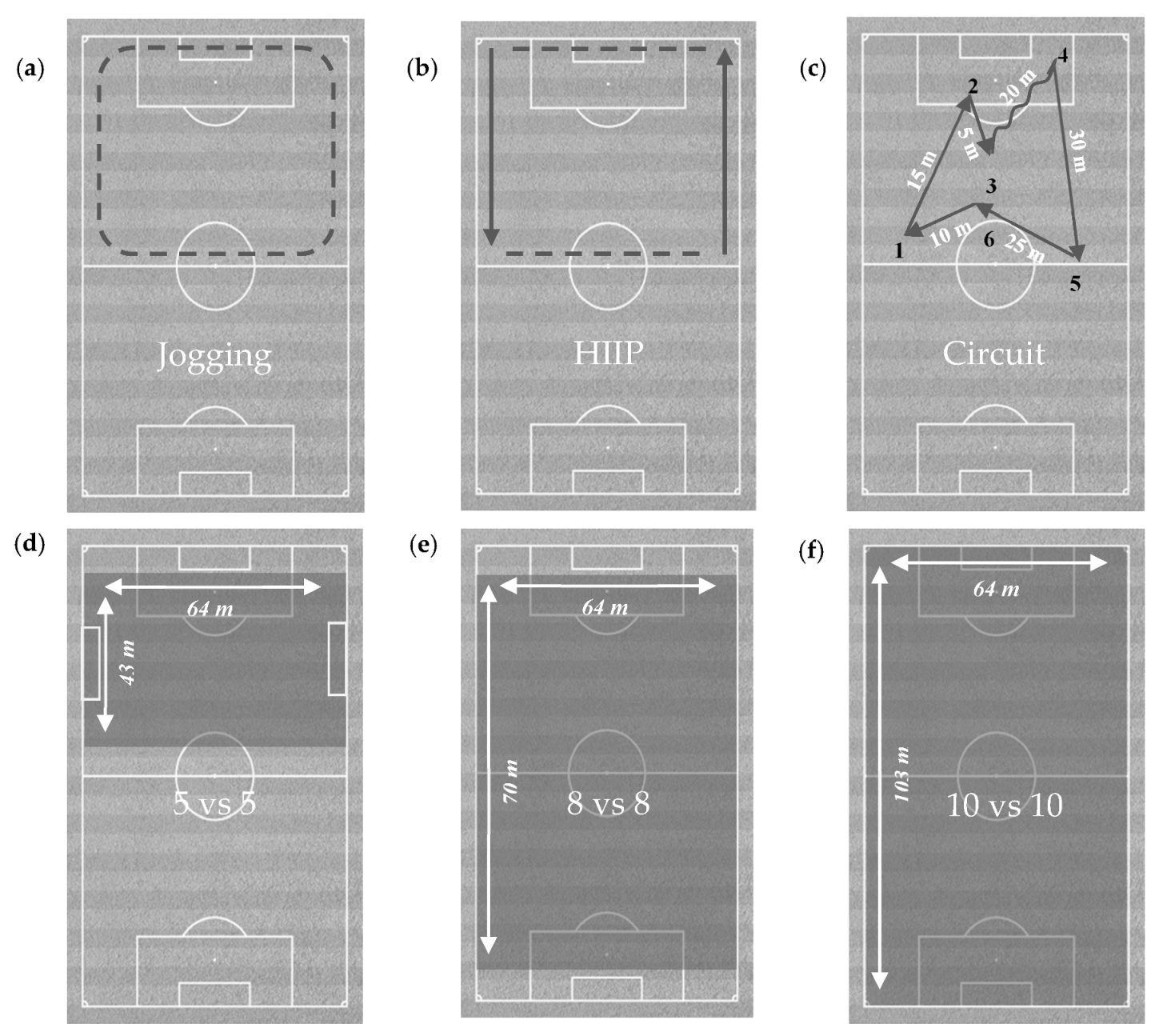
To get a comprehensive understanding of the fluctuation characteristics of player movement behavior, we investigated the multifractality of six accelerometry signals belonging to the following experimental conditions: jogging, high intensity interval protocol (HIIP), circuit running (CR), 5 vs. 5, 8 vs. 8 and 10 vs. 10 small-sided games (SSG), as illustrated in Figure 1. The conditions are described as follows:

• Jogging: low intensity self-paced steady state running.
• HIIP: consisting of 10 s of maximum effort of linear running interspersed with 20 s active recovery.
• RC: comprised of walking, jogging, running and sprinting. To each element was assigned a number, 1 to 4, respectively, and a sequence of numbers was randomly generated using an Excel spreadsheet. The exercise intensity was changed every 5 s according to the sequence using a verbal command.
• 5 vs. 5 SSG.
• 8 vs. 8 SSG.
• 10 vs. 10 SSG.

The small-sided games were played in a pitch area proportional to the number of players on small (43 m × 64 m), medium (70 m × 64 m) and large (103 m × 64 m) fields, respectively. The activities of jogging, HIIP and RC were 5 min long. The small-sided games were 10 min long and the initial and final 2 min 30 s were rejected for analysis, avoiding adaptation to the task and fatigue issues, thus leaving 5 min for analysis. Prior to each data collection, participants received proper instruction regarding the execution of the task and subsequently performed a standardized warmup consisting of 5 min of calisthenics and active stretching, followed by 5 min of jogging.

2.3. Data Processing

All signals were analyzed in raw format and no pre-processing technique was employed. To investigate the multifractal features of the data, the Discrete Wavelet Leader analysis of the accelerometry signal was computed using MATLAB software (MathWorks© 2019b). A biorthogonal wavelet “bior1.5” was used as the mother wavelet function. The maximum decomposition level was set to log₂ of the sample size (signal length). The regression type was set to “uniform”, which means that the leader coefficients were uniformly weighted in all decomposition levels. The range of statistical moments (q-moment) used varied from −5 to +5.

2.4. Multifractal Discrete Wavelet Leader

The discrete wavelet leader (DWL) is an analytical technique rooted in signal processing that provides a unity of approach to the multifractal analysis complex signals [21]. The DWL deals well with nonstationary, heterogeneous and transient behavior, therefore, it can be useful for analyzing a range of complex signals. The DWL is a nonparametric method and requires no previous knowledge about the system that will be under study.

Essentially, the DWL aims to characterize the fluctuations of the time of the local singularity in a signal $x\left[t\right]$ or function $f\left(t\right)$ by quantifying the size of the sets of points in ${\mathbb{R}}^d$, sharing a same local singularity $h$. Local singularity can be quantified by pointwise exponents, the most common one being the Hölder exponent, $h_f\left(t_0\right)$, defined as follows:

$f$ belongs to $C^{\alpha }\left(t\right)$, $\alpha \ge 0$, if there exists a polynomial $P_t$ with deg$\left(P_t\right)<\alpha$ and a constant $C>0$ such that: $\left|f\left(t+a\right)-Pt\left(t+a\right)\right|\le C{\left|a\right|}^{\alpha }$ when $\left|a\right|\to 0$. The Hölder exponent consists of the largest such $\alpha : h\left(t_0\right)=sup\left\{\alpha : f\in C^{\alpha }\left(t_0\right)\right\}\ge 0$.

Essentially, the larger $h\left(t_0\right)$, the smoother $f$ around $t_0$, and conversely, the closer $h\left(t_0\right)$ to 0, the more irregular $f$ at $t_0$. The wavelet leaders have shown to be, theoretically, the only multiscale measure able to characterize the Hölder exponent [22]. To describe the characteristics of a local singularity, DWL analysis relies upon the discrete wavelet transform (DWT) of a signal $X=\left\{x_k, K\in Z\right\}$, that is given by:

$$d_x\left(j,k\right)={\displaystyle \int }X\left(t\right)2^{-j}{\psi }_0\left(2^{-j}t-k\right)dt$$

(2)

where ${\psi }_0$ is the “mother” wavelet with a compact time support, $t$ is time script, $j$ is the dyadic scale parameter, and $k$ relates to the shift parameter. According to Ihlen and Vereijken [19], the DWT calculates the scale-dependent measure $d_x\left(j,k\right)$ by a recursive high and low pass filtering of the signal $X$. The authors describe the process as follows: “the scale-dependent measure $d_{j=1,k}$ is the convolution product ⊗ of the signal $x\left[t\right]$ and the high pass filter ${\psi }_t^{hi}$ subsampled by 2. Then, the subsampled convolution product ⊗ of the time series $x\left[t\right]$ and the low pass filter ${\psi }_t^{lo}$ is used in another convolution and subsample procedure to define the scale-dependent measure $d_{j=2,k}.$ The subsampling by 2 leads to dyadic intervals ${\lambda }_{j,k}$ that halves the sample sizes $j=1/2^j$ for each new level $j$, but double the frequency band $f=2^j$. The wavelet leaders are therefore defined as the local maxima of 3 subsequent intervals ${\lambda }_{j’,k}$ on scale $j’$ and for all $j<j’$, as follows” [19]:

$$L_x\left(j,k\right)=su{p}_{\lambda ‘\in 3\lambda }\left|d_x\left(j.k\right)\right|$$

(3)

The size and variability of the sets of points where the pointwise singularity exponent takes a given value $h$ is mathematically formalized as the Hausdorff dimension $D$ [23], which encapsulates the Hausdorff dimensions of the sets of points where a pointwise singularity exponent takes a given value $h$. The Legendre formalism describes the multifractal spectrum $D\left(h\right)$ indirectly by the $q$-order statistical moment $S\left(j,q\right)$ of the local scale-dependent measure $L_X\left(j,k\right)$. Then, for a signal $X$, let $S\left(q,j\right)$ denote the structure function and $\zeta \left(q\right)$ the scaling exponents, where $q$ is the order (or moment) of multi-resolution. They are expressed as follows:

$$S\left(j,q\right)=\frac{1}{n_j} {\displaystyle \sum }_{k=1}^{n_j}{\left|L_X\left(j,k\right)\right|}^q$$

(4)

$$\zeta \left(q\right)=\underset{j\to 0}{\lim } inf\left(\frac{logS\left(q,j\right)}{j}\right)$$

(5)

where $L_X$ represents the largest wavelet coefficient calculated at all finer scales, $n_j$ is the number of leaders $L_X\left(j,k\right)$ available at scale $2^j$ defined on each scale $j$. The $q$-order mass exponent ${\zeta }_q$ is estimated by the linear regression of Equation (4) in log coordinates vs. $log\left(j\right)$ for several $q$-orders.

The $q$-order scaling exponent ${\zeta }_q$ is then Legendre-transformed into the corresponding dimension $D\left(h\right)$ by the following equation:

$$D\left(h\right)=\underset{q\ne 0}{inf}\left(1+qh-{\zeta }^L\left(q\right)\right)$$

(6)

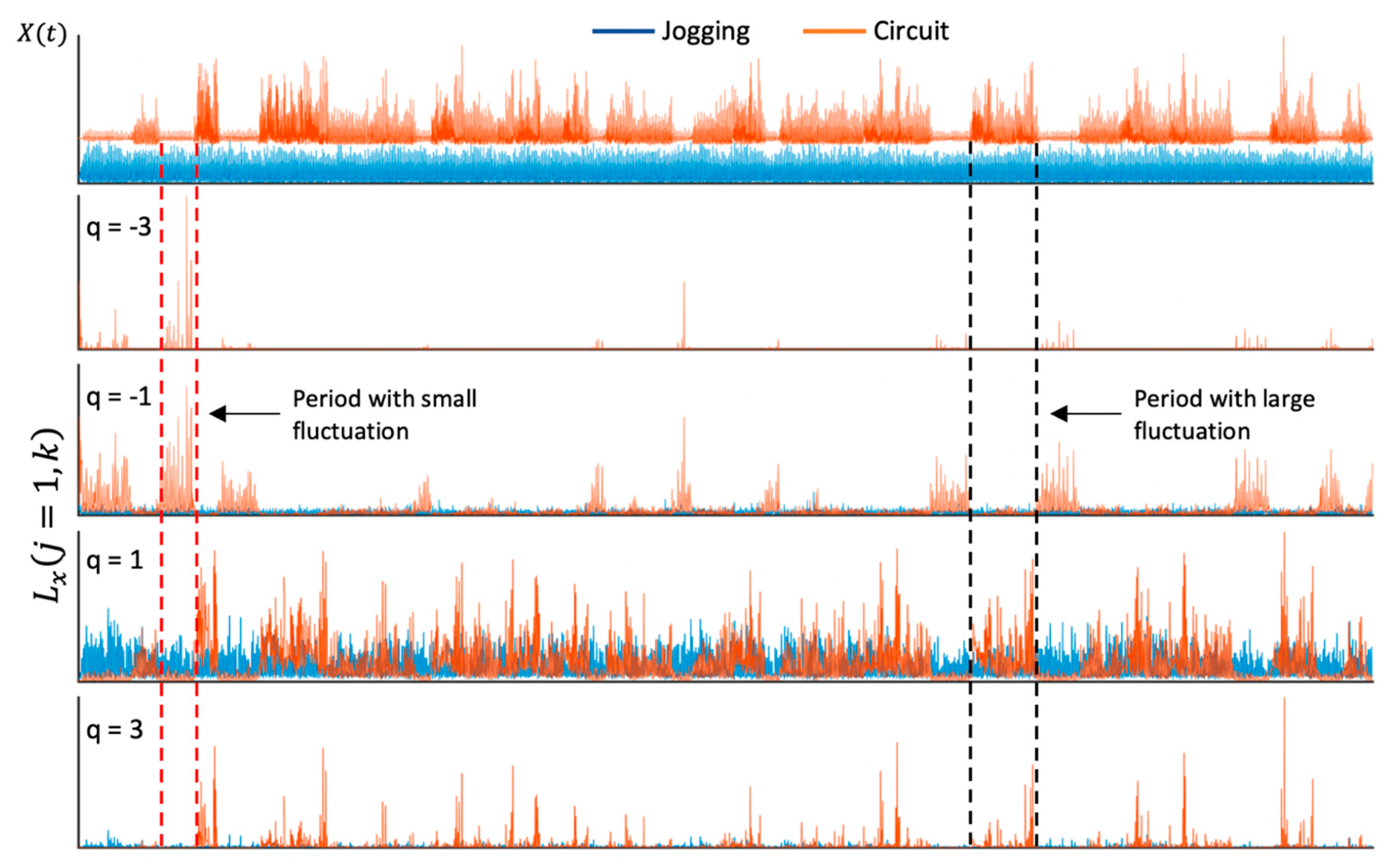
According to Ihlen and Vereijken [19], “the Legendre formalism assumes that ${\zeta }_q$ is a convex function of $q$ such that its tangent slope, the singularity exponent $h_q$, is a monotonically decreasing function of $q$. The positive $q$-orders will amplify $L_X\left(j,k\right)$ in Equation (4) for the large fluctuations in the signal whereas the negative $q$-orders will amplify $L_X\left(j,k\right)$ for the small fluctuations” (seen in the red and black intervals in Figure 2, respectively). The $q$-order’s singularity exponents $h_q$ for negative $q$ represents the right tail of the singularity spectrum whereas positive $q$ represents the left tail of the singularity spectrum. In the special case of the monofractal noise-like time series, ${\zeta }_q$ is a linear function of $q$ and, consequently, $h_q$ and $D\left(h\right)$ are $q$-independent constants collapsing the singularity spectrum $D_{h_q}$ into a very narrow support.

2.5. Interpreting the Multifractal Singularity Spectrum

This section is devoted to the explanation and interpretation of the components of the multifractal spectrum. A narrow singularity spectrum represents relative systematic fluctuations in the signal that occur over similar amplitudes over time, resembling a mono-scaling structure. A broad singularity spectrum represents more intermittent and asystematic fluctuations in the movement that occur over a greater range of amplitudes in different time lengths, a benchmark of multifractal processes. Therefore, the range of the singularity spectrum is suggested to be a measure that captures the dynamics of the system [24,25].

The singularity exponents $h$ for the large fluctuations are small and located in the left tail of the spectrum, whereas $h$ for the small fluctuations are large and located in the right tail of the spectrum. The strength of multifractality is therefore described by the large deviation of the local singularity exponent $h$ from the central tendency $h\left(0\right)$. The monofractal signal is the case when $h$ is almost constant and presents very short support, in some cases, collapsing into a single point at $h$ [19].

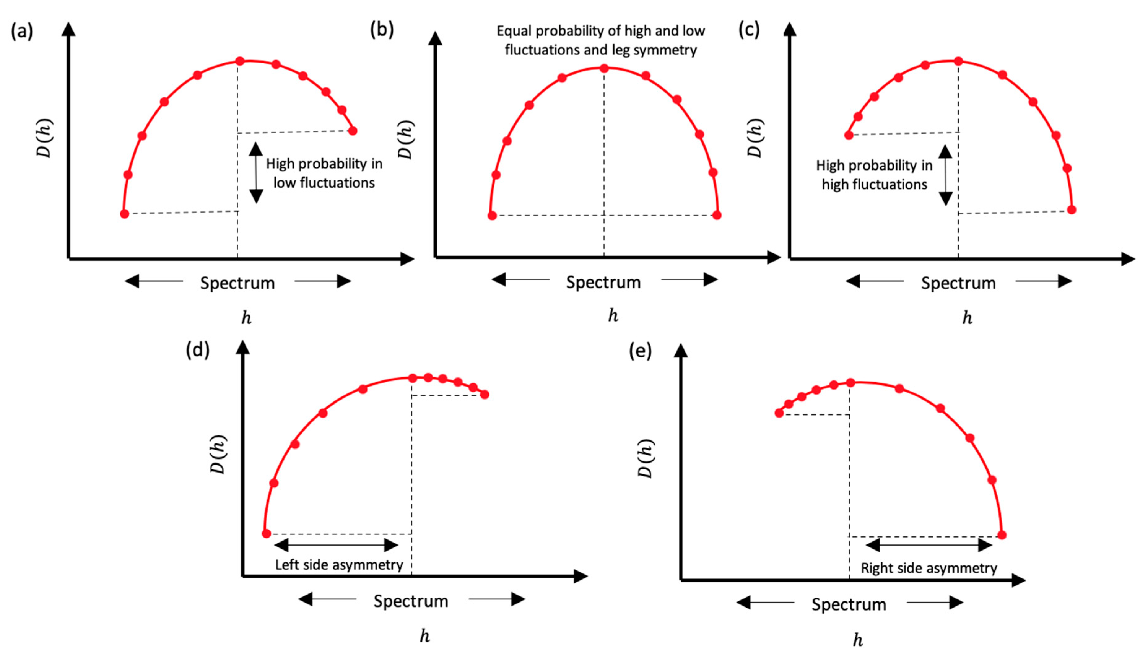
The range $h$ indicates the variety of singularity exponents that describe the dynamics of the system while the value of $D\left(h\right)$ indicates the probability of the contribution of a respective $h$.

Following this, the range of a singularity spectrum is subdivided into a left limb $\left(L\right)$ and a right limb $\left(R\right)$ (Figure 3), related to the dynamics of the highest and lowest fluctuations, respectively. The asymmetry degree of the multifractal spectrum can be identified using Δ$S$. If Δ$S<0$, the multifractal spectrum presents a long left tail, indicating that the structure in the time series is not sensitive to local fluctuations with small magnitudes. If Δ$S>0$, the multifractal spectrum presents a long right tail, indicating that the structure in the signal is not sensitive to the local fluctuations with large magnitude [24]. In cases where high and low fluctuation components of a signal present a similar scaling complexity, the singularity spectrum will result in being approximately symmetrical and $L=R$ [25]. In cases of more complexity in either of these components, the singularity spectrum becomes asymmetrical, resulting in one limb being broader than the other.

The nature of the higher fluctuation rate occurring with a higher probability can be interpreted using Δ$D_h$, calculated by the difference between the fractal dimensions of maximum and minimum probability subsets [24]. Therefore, if Δ$D_h>0$, “the maximal fluctuation rate occurs with a higher possibility than that of the minimal fluctuation rate, and vice versa” [24].

3. Results

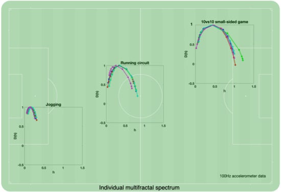
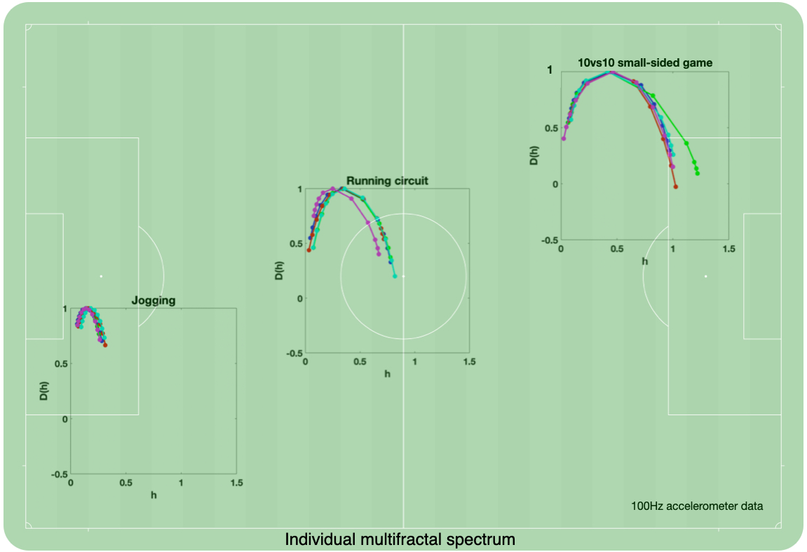
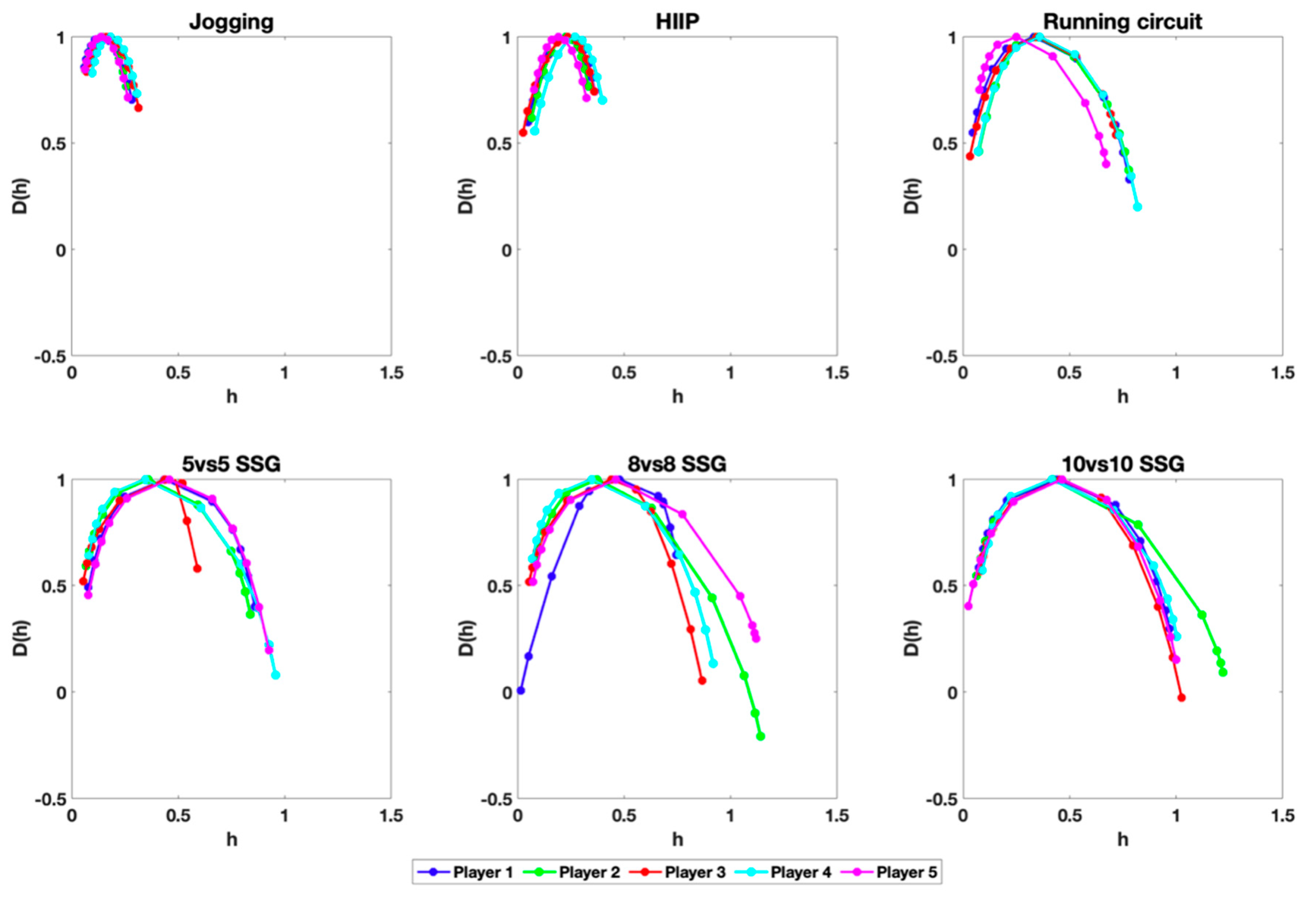
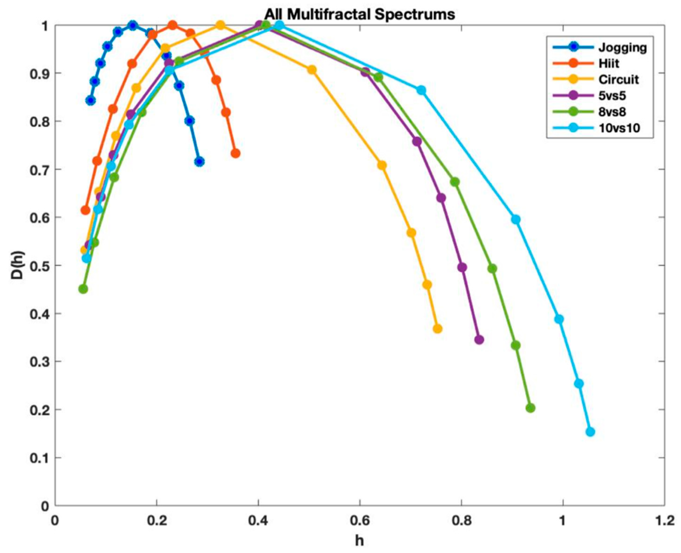
The individual multifractal spectra corresponding to all conditions are presented in Figure 4. Average values for each condition can be found in Figure 5, with additional information related to those multifractal spectra presented in

Table 1. The values of the multifractal spectrum component for each tested condition.

Components	Conditions (Mean ± SD)
	Jogging	HIIP	Circuit	5 vs. 5	8 vs. 8	10 vs. 10
$h\left(0\right)$	0.153 ± 0.018	0.231 ± 0.028	0.325 ± 0.044	0.403 ± 0.052	0.415 ± 0.055	0.441 ± 0.015
$h_{min}$	0.069 ± 0.015	0.060 ± 0.023	0.059 ± 0.020	0.068 ± 0.012	0.055 ± 0.024	0.062 ± 0.030
$h_{max}$	0.284 ± 0.025	0.355 ± 0.029	0.753 ± 0.058	0.835 ± 0.132	0.936 ± 0.161	1.054 ± 0.101
Δ$h$ $h_{max}-h_{min}$	0.215 ± 0.020	0.295 ± 0.038	0.694 ± 0.060	0.767 ± 0.121	0.881 ± 0.144	0.992 ± 0.104
$D_h\left(h_{min}\right)$	0.843 ± 0.010	0.615 ± 0.0.82	0.532 ± 0.130	0.542 ± 0.079	0.451 ± 0.254	0.515 ± 0.072
$D_h\left(h_{max}\right)$	0.717 ± 0.037	0.733 ± 0.026	0.368 ± 0.122	0.345 ± 0.185	0.203 ± 0.278	0.154 ± 0.136
Δ$D_h$ $D_h\left(h_{max}\right)-D_h\left(h_{min}\right)$	−0.126 ± 0.039	0.118 ± 0.091	−0.164 ± 0.176	−0.197 ± 0.211	−0.248 ± 0.494	−0.361 ± 0.146
$L=h\left(0\right)–h_{min}$	0.084 ± 0.005	0.171 ± 0.037	0.266 ± 0.054	0.335 ± 0.054	0.360 ± 0.072	0.380 ± 0.035
R =$h_{max}-h\left(0\right)$	0.131 ± 0.017	0.124 ± 0.011	0.428 ± 0.035	0.432 ± 0.0141	0.521 ± 0.185	0.612 ± 0.0112
Δ$S=R-L$	0.047 ± 0.016	−0.047 ± 0.041	0.162 ± 0.069	0.161 ± 0.069	0.162 ± 0.240	0.232 ± 0.129

.

The mean generalized Holder exponent $h\left(0\right)$ for each of all six conditions reveled values less than 0.5. By definition, this means that all six conditions presented long memory with anti-correlated behavior.

Analysis among the width of the multifractal spectrum Δ$h$ revealed a trend between the condition performed and the width of the multifractal spectrum. Indeed, the 10 vs. 10 SSG had the widest ($\Delta h=0.99$) and jogging (Δ$h$ = 0.21) showed the narrowest.

The mean values of Δ$D_h$ for jogging, circuit running, 5 vs. 5, 8 vs. 8 and 10 vs. 10 were all negative, meaning that the maximal fluctuation rate occurred with a higher probability than the minimal fluctuation rate, however, not for all the players. Contrarily, the mean value of Δ$D_h$ for HIIP was positive, indicating that the minimal fluctuation rate occurred with a higher probability than the maximal fluctuation rate.

The mean values of Δ$S$ for the jogging, circuit running, 5 vs. 5, 8 vs. 8 and 10 vs. 10 were all positive, indicating that multifractal spectra had long right tails, and multifractal structures were more sensitive to local fluctuations with small magnitudes, if compared to the fluctuations with large magnitudes. Conversely, the mean value of Δ$S$ for the HIIP is negative, indicating that its multifractal spectrum had a long left tail, and its multifractal structure was more sensitive to local fluctuations with large magnitudes.

4. Discussion

This study aimed to explore the multifractal features of football players’ movement behavior using accelerometry measures by means of the discrete wavelet leader method. Overall, our exploratory results revealed a strong trend between the task and the shape and size of the multifractal spectrum. Indeed, more complex tasks led to wider multifractal spectrums while less complex tasks resulted in narrower multifractal spectrums. The increment in task complexity reshaped the multifractal spectrum most often systematically by stretching its right leg to the right assuming long-range positive correlations in lower fluctuations, whereas, the left end of the spectrum remained almost unchanged. This means that the analysis was sensible in capturing small fluctuations but ineffective in capturing larger fluctuations. Since the $h_{min}$ for jogging was already very small at the beginning $h_{min}=0.069$, it became harder to detect greater fluctuations in accelerometry. In conjunction, the high-pass wavelet filter appeared to have an inferior resolution than what was required to capture the high fluctuations, however, it performed considerably well on small fluctuations.

Comparing the values of the Hausdorf dimension of pointwise singularities $D\left(h\right)$ for each condition demonstrates that the maximal fluctuations were associated with more probability in all tasks if compared to the small fluctuations, with the exception of HIIP. Indeed, the work-to-rest ratio (i.e., work 1:2 rest) used in the HIIP protocol clearly emphasized a longer duration for low fluctuations (rest) during the activity, thus, conferring more probability if compared to higher fluctuations.

Interestingly, the dynamics of SSG showed a similar pattern for the left leg of the spectrum, almost superimposing its components. This may suggest that the periods with large fluctuations behave similarly among these conditions. Contrarily, the right leg of the spectrum stretched to the right with an increase in the number of players and field dimension, which seems reasonable since players may experience more periods with lower intensity (walking or standing). The summation of this behavior turned out to make the signal uncorrelated, which corroborates with the increase of $h\left(0\right)$ values from anti-correlated to no correlation.

The multifractal spectrum (width and shape) could reflect the adaptability of movement to external variation and shown the characteristic configuration for each activity. Adopting a similar approach Fuss, Subic [23] explored the Hausdorff dimension along with the average amplitude of the acceleration signal to identify wheelchair rugby accelerations among different activities. The results showed that Hausdorff dimension values of high speed pushing and high speed coasting were similar, and also show the average amplitude values of collisions and high speed pushing. In addition to this first exploration, it seems clear that the multifractal analysis of the movement behavior of the football players introduces a complementary dimension to the research of performance and coordination of human behavior in dynamic environments. In fact, the close relation between stochastic processes and movement behavior makes multifractal analyses an innovative and promising candidate tool for investigation.

Future studies might consider different parameters for the wavelet leader analysis, such as the wavelet type and the number of decomposition levels, as well as pre-processing techniques, such as filtering. It is important to highlight that the wavelet leader multifractal analysis is very sensitive to any of the above-mentioned conditions.

The jogging activity showed the narrowest multifractal spectrum, resembling a monofractal structure, with a $h$ value centered at 0.15, which indicates an overall long memory anticorrelated behavior. Indeed, jogging is a stationary activity with regular fluctuations that might change due to inherent attributes of motor control (variability of movement) if compared to changes imposed by the task. The elevated value of $D\left(h\right)$ in the left end of the spectrum indicates that the high fluctuations present more probability throughout the signal if compared to low fluctuations.

The HIIP activity showed a multifractal spectrum with an $h$ value centered at 0.23, which indicates overall long memory anticorrelated behavior and a larger range of singularity exponents than the jogging activity. In HIIP, the players had to perform all-out accelerations causing tremendous rise in the amplitude of the accelerometry signal while maintaining jogging during resting. Consequently, the spectrum of singularities indicates higher fluctuations if compared to the jogging activity with a lower probability if compared to low fluctuations.

With the exception of player 5 who showed symmetry and almost equal probability of large and small fluctuations, all spectrums show a long left leg $\left(R<L\right)$—an aspect that can be attributed to the change in high intensity running and maintenance of small fluctuations $D_h\left(h_{max}\right)>D_h\left(h_{min}\right).$ The fact that the low fluctuations were shifted a little to the right might indicate that adaptations in the rest period, to balance the effects of fatigue, made the fluctuations while jogging less anti-correlated, or less noisy.

The circuit activity showed a larger multifractal spectrum than jogging and HIIP activities. That was the first case an activity spectrum started to show positive correlations. This might have happened due to the inclusion of walking, which created a positive correlation in the spectrum. Clearly walking introduces a new pattern of behavior with very low fluctuation in its signal dynamics. Except for player 3, all spectrums showed a long right leg $\left(R>L\right)$ and suppression of small fluctuations over large fluctuations $D_h\left(h_{max}\right)<D_h\left(h_{min}\right)$, suggesting a higher probability of jogging, running and sprinting than walking.

The 5 vs. 5 SSG showed a multifractal spectrum with an $h$ value centered at 0.40 which indicates an overall anticorrelated behavior very close to no correlation. Its range of singularity spectrums indicates richer fractality if compared to jogging, HIIP and circuit running, but it performed the poorest in the SSGs. The individual analysis demonstrates different behavior among players with some characterized by long memory with anti-correlation $h <0.5$ (i.e., players 2 and 4) and others characterized with no correlation $h=0.5$ (i.e., players 1, 3 and 4). With the exception of player 3, all spectrums show a long right leg $\left(R>L\right)$ and suppression of small fluctuations over large fluctuations $D\_h \left(h\_max \right)<D\_h \left(h\_min\right)$.

The 8 vs. 8 SSG showed a multifractal spectrum with an $h$ value centered at 0.41 which also indicates an overall anticorrelated behavior very close to no correlation. The individual analysis demonstrates different behaviors among players with some characterized by long memory with positive-correlation $h<0.5$ (i.e., player 1), anti-correlation $h<0.5$ (i.e., players 2 and 4) and no correlation $h=0.5$ (i.e., players 3 and 5). All spectrums presented wide support. Players 2, 4 and 5 demonstrated long right leg $\left(R>L\right)$ with suppression of small fluctuations over large fluctuations $D_h\left(h_{max}\right)<D_h\left(h_{min}\right).$ Players 1 and 3 showed long left leg $\left(R<L\right)$, and, while player 1 showed suppression of large fluctuations over small fluctuations $D_h\left(h_{max}\right)>D_h\left(h_{min}\right)$, player 3 showed the opposite results.

The 10 vs. 10 SSG showed a multifractal spectrum with an $h$ value centered at 0.44 which also indicates an overall anti-correlated behavior very close to no correlation. The singularity spectrums are characterized by the largest among all conditions. All spectrums show a long right leg $\left(R>L\right)$ and suppression of large fluctuations over small fluctuations $D_h\left(h_{max}\right)<D_h\left(h_{min}\right).$

5. Conclusions

The wavelet leader multifractal analysis has shown to provide different insights into the analysis of complex signals in sports performance scenarios. However, more research is needed to explore improvements in the analysis and ways of implementation of this information in the training setting. Although the systematicity presented in the current study leveraged new and fruitful information for the analysis of movement behavior in football, the transfer to training is still a shortcoming. The use of asymmetry parameters, such as Δ$D_h$, Δ$h$ and ΔS, may be a good starting point to explore the demands of training sessions, allowing comparisons among players and providing substance to support different research questions. The current results are exploratory and might be limited by the sample expertise level, however, the experiment has the potential to be used in understanding several key performance questions, namely: (i) collective synergies, (ii) talent development and (iii) pre- to post-injury changes.