Article

Multi-Classifier Approaches for Supporting Clinical Decision Making

de Health Lab-Laboratory of Decision Engineering for Healthcare Services, Department of Mechanical, Energy and Management Engineering, Ponte Pietro Bucci 41C-University of Calabria, 87036 Rende, Cosenza, Italy
*
Author to whom correspondence should be addressed.
Symmetry 2020, 12(5), 699; https://doi.org/10.3390/sym12050699
Submission received: 26 March 2020 / Revised: 18 April 2020 / Accepted: 26 April 2020 / Published: 1 May 2020
(This article belongs to the Special Issue Optimized Machine Learning Algorithms for Modeling Dynamical Systems)

Abstract

:
Diagnosis is one of the most important processes in the medical field. Since the knowledge domains of clinical specialties are expanding rapidly in terms of complexity and volume of data, clinicians have, in many cases, difficulties to make an accurate diagnosis. Therefore, intelligent and quantitative support for diagnostic tasks can be effectively exploited for improving the effectiveness of the process and reduce misdiagnosis. In this respect, Multi-Classifier Systems represent one of the most promising approaches within Machine Learning methodologies. This paper proposes a Multi-Classifier Systems framework for supporting diagnostic activities with the aim of improving diagnostic accuracy. The framework uses and combines several classification algorithms by dynamically selecting the most competent classifier according to the test sample and its location in the feature space. Here, we extend our previous research. The new experimental results, compared with several multi classifier techniques, based on dynamic classifier selection, on classification datasets, show that the performance of the proposed framework exceeds the state-of-the-art dynamic classifier selection techniques.

1. Introduction

The diagnosis process has a remarkable impact within the medical sector, due to the wide scope and complexity of clinical knowledge domains. In general, diagnosis is a dynamic process in which clinicians have to process various types of data, e.g., signs and symptoms, vital parameters that vary over time, biomedical and clinical data, results of instrumental and laboratory tests, results of imaging devices, in order to accurately detect a specific disease. Since the amount of data and information to be processed is typically rather high, computerized systems based on Machine Learning (ML) classification techniques can be effectively exploited for improving the effectiveness of diagnosis processes and reduce misdiagnosis. With ML, the diagnostic process (basically a classification task) is represented and analysed on the basis of retrospective observed data by exploiting an inductive approach.
Generally speaking, classification is the process of predicting the category of given data points. A classifier is a function that can perform classification task.
In detail, let D = x 1 , x 2 , , x n be a dataset with n instances denoted by x i , i = 1 , 2 , , n . Each instance x i = { a 1 , a 2 , , a m , y k } consists of m attributes and a class label y k from a finite set of disjoint labels y = y 1 , y 2 , , y k . Let x i * be a test instance; a classifier returns the class label predicted for x i * .
A Multi-Classifier System (MCS) is a system that uses different classifiers with the aim to obtain better results in a classification task by exploiting the single classifier competences [1,2].
The development of an MCS involves three phases: generation, selection and integration. In the generation phase, a pool of several classifiers, which are called base classifiers, is trained using a training set. The classifiers in the pool must be characterized by different performance, since it does not make sense to combine classifiers that provide the same accuracy in the prediction. Different strategies have been proposed in the literature to generate a diverse pool of classifiers: classifier of different types, different architectures, different features, different training sets, different parameters for each classifier [3]. In the selection phase one or a subset of the base classifiers is selected based on an appropriate selection criterion. Dynamic Ensemble Selection (DES) techniques select more classifiers for the classification of each test instance [4,5] whereas Dynamic Classifier Selection (DCS) techniques select a single classifier [2]. Finally, in the integration phase a decision is made based on the predictions of the selected classifiers.
Two approaches of classifier selections have been proposed in the literature: static and dynamic [6]. MCS based on a static classifiers selection exploits the same classifier to classify any test instances. MCS based on dynamic selection instead, selects a specific classifier to classify each test instance, due to the assumption that each base classifier is an expert in a different local region. The local region consists of labelled instances located near to a given test instance and the most appropriate classifier in the local region is selected according to a given competence criterion. The key issues in Dynamic Selection (DS) are (1) how to define the local region and (2) how to estimate the competence of the base classifiers.
In many DS approaches, the local region is constructed using the k-Nearest Neighbour (k-NN) algorithm where k is a static parameter [7,8,9,10] defined through computational experiments. With a static value of k the local region has the same size for each test instance. Several versions of the k-NN algorithm have been proposed to improve the construction of these regions where k is a static parameter for the algorithm as reported in the survey presented in [3]. Some works proposed the use of adaptive region that changes according to the test instance. In [11] the k parameter of the k-NN algorithm is selected according to the output of the classifier. For a given classifier C j and a given k, if there is no instance in the local region belonging to the same class assigned to the test instance, the value of k is increased.
However, these approaches does not take into account where the instances are located and therefore how far they are from the test instance.
Several criteria are used for estimating the competence level of the base classifiers mainly based on accuracy [9], ranking of classifiers [12], probabilistic information [7], classifier’s behaviour [8], oracle-based measures [13], diversity measures [14], ambiguity-based measures [15].
In this paper, we propose a general MCS framework based on DCS in order to improve the accuracy of diagnostic process. The novelty of the proposed approach is based on: (1) the local region of each test instance is defined dynamically; (2) the most competent classifier is selected by a procedure based on performance indexes evaluated on both local region and a specific set of instances. We further extend the preliminary results appeared in [16]. By computational experiments carried out on clinical datasets, we compared the proposed MCS framework with state-of-the-art DCS techniques, namely Overall Local Accuracy (OLA) and Local Class Accuracy (LCA) [3,6,9]. A statistical analysis was performed using the Wilcoxon signed rank test.
Among the DCS techniques, OLA and LCA display the best performances [3]. OLA evaluates the accuracy of each base classifier as the percentage of correct labelled instances in the local region. The classifier that gets the highest accuracy is considered the most competent. LCA evaluates the accuracy of each base classifier of a single class. In this case, the accuracy is defined as the percentage of correct labelled instances in the local region belonging to the class assigned by the classifier to a given test instance. Even in this case, the classifier that gets the highest accuracy is considered the most competent. In both cases the local region is defined during the testing phase by the static k-NN algorithm and only one classifier is selected to perform the classification task.
The paper is organized as follows. In Section 2, we describe and motivate the proposed MCS framework. Experimental results and relevant discussion are detailed in Section 3, by considering representative clinical diagnosis decision-making problems. Some conclusions are sketched in Section 4.

2. Proposed MCS Framework

The proposed MCS framework follows the general pattern of a supervised classification process (i.e., the class label of data is known).
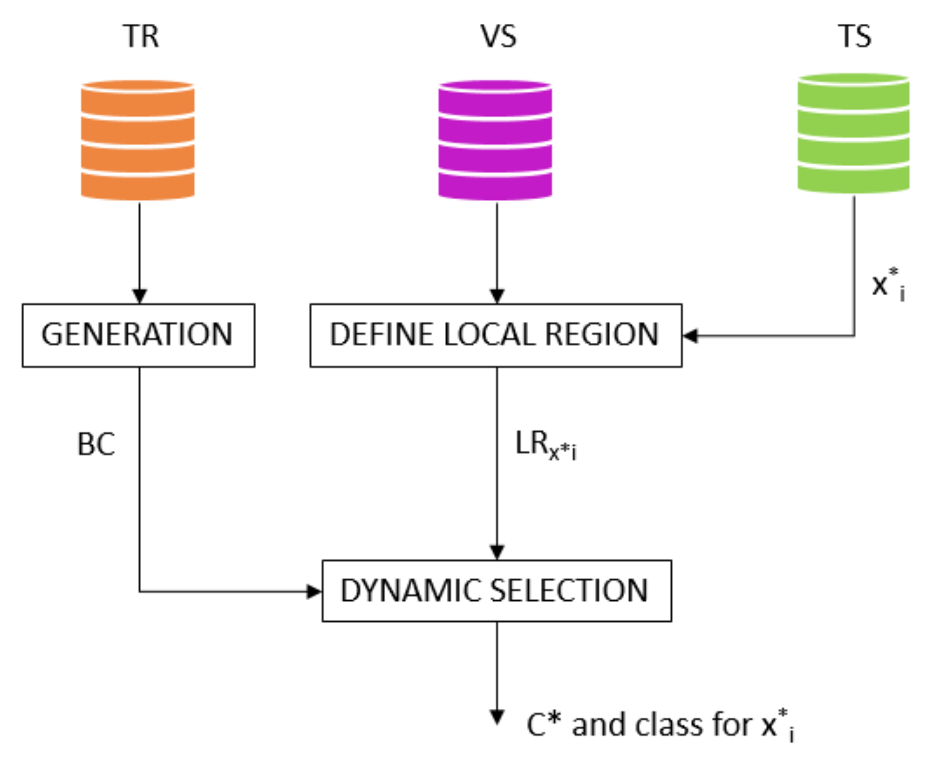
A dataset is split into three disjunctive sets, i.e., training set, validation set, and test set, which are denoted by TR, VS, and TS, respectively. The training set is used to train classifiers; the validation set is used to estimate classifiers’ ability to recognize new instances; finally, a test set contains instances that have to be labelled by the trained classifiers and it is used to estimate the classifier accuracy. Let B C = c 1 , c 2 , , c k , be a pool of k base classifiers, which are denoted by c j , j = 1 , , k . Let x i * , be a test instance. The MCS framework consists of three main phases:
  • Generation The pool of base classifiers B C is generated and they are thus trained on instances of T R . As we show in Section 3, a pool contains diverse classification ML algorithms in order to provide a broad coverage of problem space variability and improve thus performance
  • Definition of the local region The local region L R x i * of a test instance x i * T S is constructed as set of neighbours in V S of x i * . An adaptive k-NN algorithm selects a given number of neighbours in V S by considering a hypersphere centered in x i * and with radius R that is defined in Equation (1). The Euclidean norm is used for the distance between x i * and instances in V S .
    R = R m a x R m i n 2 i f R m a x > 3 R m i n R m i n o t h e r w i s e
    where R m a x and R m i n are the maximum and the minimum distance, respectively, between x i * and all other instances in the validation set.
    The radius R of the hypersphere is set to R m a x R m i n 2 if R m a x R m i n 2 > R m i n , from which R m a x > 3 R m i n .
    Therefore the radius of the hypersphere is set as R m a x R m i n 2 i f R m a x > 3 R m i n otherwise, the radius would be less than R m i n and the local region would be empty. For this reason we set R = R m i n when the condition is not verified, that is, when R m a x 3 R m i n .
    Depending on Equation (1), the radius of the smallest hypersphere is R m i n whereas that one of the biggest hypersphere is R m a x 2 , which occurs when R m i n is close to zero.
    The idea behind the adaptive k-NN algorithm is to consider only instances that are really close to x i * in the original features space. If R = R m i n , the local region could contain only one instance. When the local region is made up of only one instance, x i * can be found in a low-density region.
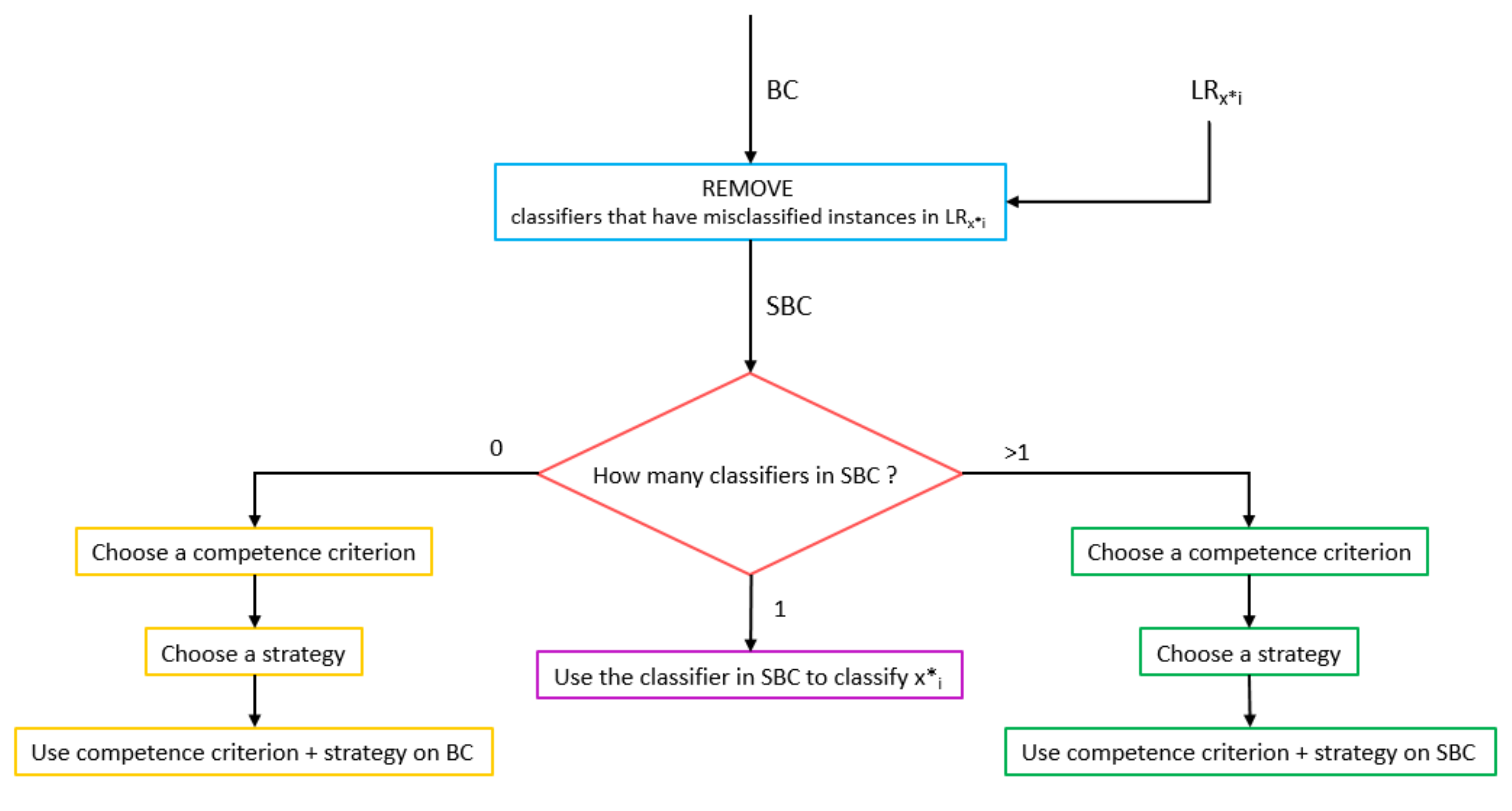
  • Dynamic Selection The most competent classifier C * for each x i * T S is selected. This phase selects locally the most competent classifier for a given test instance x i * . The overall selection process is based on performance indexes evaluated both on a local region and a specific set of instances. The selection procedure consists of two stages: Firstly, classifiers’ competence is evaluated on local region L R x i * . In order to select the most competent classifier, those ones that misclassify instances in L R x i * are removed. The subset of remaining classifiers is denoted by S B C B C . Then, the classifiers are assessed using different data sets according to the current situation.
    Figure 1 show the steps of the selection phase based on the cardinality of the set S B C . The three possible cases are detailed in the following.
    case 1 :
    S B C = , that is, all base classifiers misclassify instances in L R x i * . The most competent classifier is thus selected among the base classifiers in the original pool B C .
    case 2 :
    S B C = 1 , only one base classifier remains in S B C and it is used to classify x i * .
    case 3 :
    S B C > 1 , that is, more than one base classifier remain and the most competent classifier is selected among them.
    Case 2 is the simplest because there is only one classifier. For Case 1 and Case 3, it is necessary to choose a competence criterion and a strategy to resolve the indeterminacy, as described in the following. We design two criteria based on recall and accuracy, respectively, and two strategies based on training and validation results, and only on validation results, respectively. We remind that Recall is the percentage of instances belonging to a given class and correctly classified; Accuracy is defined as the percentage of instances correctly classified.
    • Criterion based on recall Let y k , be the class of majority instances in L R x i * . The recall of the classifiers is evaluated on instances of the class y k ; thus, classifier with the highest recall is selected
    • Criterion based on accuracy The classifier with the highest accuracy is selected. In this case, we do not consider a specific class
    • Strategy 1 (validation and training results): one of the two above defined criteria is chosen. The criterion is thus firstly applied to evaluate classifiers on the validation set. If there is indeterminacy because more classifiers have the same performance index value, the criterion is applied on the training set. More specifically, the criterion is applied on the training set only for the classifiers with the same performance. If there is indeterminacy again, the mean absolute error (MAE) on the training set is evaluated and the classifier with the minimum MAE is selected. The MAE is calculated on all training instances.
    • Strategy 2 (validation results): one of the two above defined criteria is chosen. The criterion is firstly applied to evaluate classifiers on the validation set. If there is indeterminacy, the MAE of each classifier is evaluated on the validation set and the classifier with the minimum MAE is selected. In this case, the MAE is computed on all VS instances
An overview of the MCS framework is depicted in Figure 2.

3. Computational Experiments

In order to evaluate the proposed MCS framework, we designed three algorithms. Algorithm 1 is based on Strategy 1; Algorithm 2 is based on Strategy 2, and Algorithm 3 is a hybrid version of the two previous ones. Observe that Algorithm 3 is reduced to Algorithm 1 when the removal step leads to Case 1, and to Algorithm 2 when the removal step leads to Case 3.

3.1. Datasets Description

We tested the three algorithms with both selection strategies on six datasets available at the UCI Machine Learning Repository [17]. These datasets have been widely used for academic research and are related to some important diagnostic problems.
Cleveland database is used to diagnoses the presence of heart disease. Wisconsin Diagnosis Breast Cancer (WDBC), Wisconsin Breast Cancer (WBC) and Mammographic mass datasets are used to diagnose the severity (benign or malignant) of a breast mass. Diabetic retinopathy dataset is used to predict whether a diagnostic image contains signs of diabetic retinopathy. Dermatology dataset is used for differential diagnosis of erythemato-squamous diseases: psoriasis, seboreic dermatitis, lichen planus, pityriasis rosea, cronic dermatitis, and pityriasis rubra pilaris. Table 1 summarizes the main characteristics of these datasets in terms of number of instances, number of attributes and number of classes.

3.2. Pool of Base Classifiers

Among the several machine learning algorithms, we choose Support Vector Machines (SVM) [18], Multi-Layer Perceptron (MLP) [19], Naive Bayes (NB) [20], Decision Tree (DT) [21], and k-NN [22], as they are widely used in different classification problems. For each classifier, we used the related algorithm implemented in Weka [23]. For this reason, in the next tables we refer to SVM as SMO (Sequential Minimal Optimization), and to k-NN as Ibk (Instance-based method with parameter k).
For SVM, we used polynomial kernel and Gaussian kernel. The MLP contains one input layer, one hidden layer, and one output layer; the number of neurons in each layer is specified by I, H and O, respectively. All of the nodes use a standard sigmoid activation function. The MLP was trained using error back-propagation algorithm, with a learning rate L, a momentum M, a training time (epochs) of 500, and a back size of 100. Moreover, for DT we used the J48 classifier that implements the C4.5 algorithm. The tuning of specific classifier parameters was carried out on each dataset in order to find the best parameter values. These used best values are in Table 2.
As the performance of the proposed framework depends on the base classifiers in the pool, we have combined and then tested pools with two, three and four base classifiers. The overall number of pools is 25. The proposed MCS framework was implemented in Java.

3.3. Performance Evaluation

The results that we details in the following tables were found by employing the stratified ten-fold cross validation (10-fold CV) method. A dataset is randomly partitioned into ten subsets and then one subset is selected for validation and testing and the remaining nine subsets for training. The whole process is repeated ten times to avoid the possible bias during dataset partitioning for cross-validation. The final results in terms of mean classification accuracy were computed by averaging the ten results. The classification accuracy is computed as reported in Equation (2), where N c o r r is the number of instances correctly classified by a given approach and N is the total number of instances.
A c c u r a c y = N c o r r N × 100
Each dataset was then divided by a stratified 10-fold CV (1-fold for testing and validation, 9-fold for training) followed by a stratified 2-fold CV (the test fold was divided into 1 fold for validation and 1 fold for test). All data were normalized and no attribute selection was performed.
The proposed MCS approaches are compared with OLA and LCA techniques. For a fair comparison, we used local regions as defined in Section 2 even for these two techniques.

3.4. Results and Discussion

The aim of the carried out computational experiments is to evaluate the proposed MCS framework and assess whether the proposed approaches improve the classification task compared to other techniques in the literature. To this end, we have considered the three algorithms above introduced, namely, Algorithm 1, Algorithm 2 and Algorithm 3. We discuss then the gain in terms of accuracy of these approaches.
Table A1, Table A2, Table A3, Table A4, Table A5 and Table A6 list the average accuracy evaluated by a 10-fold CV on the six datasets for every algorithm. There are thus 25 × 9 accuracy values in each table. The relevant implementation for each algorithm is even specified, that is, if the selection criterion is based on recall (CR) or accuracy (CA). The tables also show the accuracy of OLA and LCA techniques. The best results for every pool of base classifiers are in bold in each row and standard deviation is shown in parenthesis. The algorithms that exceed OLA and LCA appears with a “*” marker.
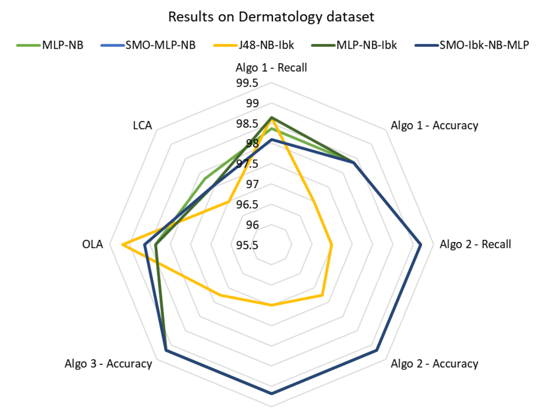
We can observe that the performance of a pool is problem dependent and that our approaches outperform OLA and LCA techniques in most cases. On Cleveland dataset, for instance, the accuracy of our approaches is better than that one found with OLA and LCA in 15 pools, and that Algorithm 1 and Algorithm 3 achieve the best performance with a mean accuracy of 85.15 %. On WDBC they exceed the OLA and LCA techniques in the majority of pools (21 pools out of 25). On the Dermatology dataset, the highest classification accuracy is 99.18 % that is achieved by several pools and the classification accuracy of both OLA and LCA techniques in 15 pools and with Algorithm 2 and Algorithm 3. These two approaches have the same performance on this dataset. We investigated this aspect and we found that the removal step produced Case 3 always (see Section 2).
Table 3 reports the best accuracy value per each dataset and specifies the corresponding pool by which this value was found.
For WDBC and Dermatology dataset there is a set of pools that found the same best value, i.e., six pools on WDBC dataset, and five pools on Dermatology dataset. The accuracy values found by the five pools on Dermatology dataset with all algorithms are compared in Figure 3.
More details can be found in Table A1, Table A2, Table A3, Table A4, Table A5 and Table A6, where the best couple pool-algorithm is in grey colour.
In order to compare the algorithm among them, we compute the average mean accuracy on the six datasets for every algorithm and evaluated on all pools, as shown in Table 4. The best results for each dataset are highlighted in bold. Based on these results, we can see that the proposed algorithms achieved the best average accuracy on all datasets.
The computational experiments show that the proposed approaches are more inclined to select the best classifier in the pool compared to OLA and LCA techniques when the same technique is used to generate the local region. Under this respect, we remark that considering the same local region, the proposed approaches outperform the OLA and LCA techniques in many cases in all datasets.

3.5. Statistical Analysis

To compare performances of the pools we perform a statistical comparison [24]. More specifically, we compare the pools accuracies using the Wilcoxon signed-ranks test [25] with α = 0.05 . We are trying to reject the null-hypothesis that both pools of base classifiers perform equally well. To simplify the interpretation of the results, we refer to a given pool by its position as they are listed in the first column of the tables of results, in the Appendix section. Moreover, we choose to analyse the performance of the pool with high accuracy and lower number of base classifiers. This statistical analysis has been carried out per each dataset and it is detailed and summarised in Table 5, where we report per each dataset the chosen pool of base classifier, the p-value range that attests a significant difference with all other pools except to those listed in the last column of the table. Analysing, for instance, the accuracy values related to the Cleveland dataset, we found that the pool IbK-SMO, which has the best accuracy value if we do not consider SMO-Ibk-NB with OLA technique (i.e., pool 11), is significantly better than all other pools of base classifiers except to the pools { 1 , 10 , 11 , 12 } because there are no significant differences. The found p-value range of the pools with significant difference is 0.007–0.042. A similar significance have the other data reported in Table 5.
For a better comparison of the proposed algorithms with OLA and LCA techniques, we conducted a pairwise test using the Wilcoxon Sign Test with a significance level of with α = 0.05 . We compare the classification accuracies of the pools for every method per each dataset. The results of the performed Wilcoxon Sign test can be summarised as follows:
  • Algorithms vs. LCA
    • All the proposed algorithms significantly exceed LCA on Dermatology, Diabetic retinopathy and WDBC datasets with a p-value between 0.0002 and 0.01935.
    • Algorithm 2 (CR and CA versions) significantly outperforms LCA on WBC dataset with a p-value of 0.01168 and 0.00196, respectively
  • Algorithms vs. OLA
    • The proposed algorithms are statistically equivalent to OLA on Cleveland, WBC and Dermatology datasets
    • Algorithm 1-CA and Algorithm 3-CA instead, significantly exceed OLA on Diabetic retinopathy dataset with a p-value of 0.04218 and 0.00120 respectively. Algorithm 2-CR instead, outperforms significantly OLA on Mammographic mass dataset with a p-value of 0.00112
    • All proposed algorithms significantly outperform OLA on WDBC dataset

4. Conclusions

In this paper, we proposed a MCS framework based on a dynamic classifier selection technique, whose novelty lies in its use on a local region dynamically computed for each test instance and a selection criterion based on both misclassified instances and information about classifier’s performance in a two-step process. In order to select the best classifier, we define three different algorithms depending on the set of instances used for compute the classifier’s performance: Algorithm 1 uses both classifier results on training and validation sets; Algorithm 2 uses only validation results; Algorithm 3 is a hybrid of the previous ones. An experimental protocol based on six datasets was performed. The computational experiments carried out with several pools of base classifiers indicate that the proposed MCS framework allows an improvement of the classification accuracy with respect to other MCS approaches.
Future works could follow two main directions. First, we could look at tuning the pools of base classifiers by evaluating different similarity metrics and different optimization parameters. Secondly, we could investigate other ML measures in order to better describe a local region.

Author Contributions

Conceptualization, M.C.G., R.G. and D.C.; Data curation, M.C.G.; Investigation, M.C.G., R.G. and D.C.; Methodology, M.C.G., R.G. and D.C.; Project administration, D.C.; Software, M.C.G.; Supervision, D.C.; Validation, M.C.G., R.G. and D.C.; Writing–original draft, M.C.G., R.G. and D.C.; Writing–review & editing, M.C.G., R.G. and D.C. All authors have read and agreed to the published version of the manuscript.

Funding

This research received no external funding

Conflicts of Interest

The authors declare no conflict of interest.

Appendix A. Tables of Results

Table A1. Classification accuracy (%) on Cleveland dataset.
Pool of Base ClassifiersAlgorithm 1Algorithm 2Algorithm 3OLALCA
CRCACRCACRCA
1NB-SMO83.17 (6.82)83.5 (6.85)83.17 (6.37)83.5 (6.85)83.17 (6.56)83.5 (6.9)84.16 (6.54)84.49 (5.82)
2MLP-SMO82.51 (6.11)83.17 (5.69) *82.51 (5.88)83.5 (5.47)*83.17 (6.11) *83.5 (5.92)*82.18 (5.68)82.84 (5.35)
3J48-SMO80.2 (6.61)81.52 (6.78) *83.17 (6.24)*82.84 (6.79)*83.83 (6.55) *82.84 (6.86)*79.87 (5.76)80.53 (5.1)
4Ibk-SMO85.15 (6.38) *84.49 (6.53) *84.82 (5.91) *84.82 (6.53) *84.49 (6.23) *85.15 (6.55) *83.17 (5.43)83.5 (4.97)
5MLP-NB81.52 (6.29)81.52 (6.86)81.52 (6.08)82.18 (6.86)82.18 (6.31)82.51 (6.89)82.18 (5.45)83.17 (5.07)
6MLP-J4881.19 (6.32) *80.53 (6.93) *81.19 (6.1) *80.53 (6.94) *80.86 (6.37) *80.53 (6.97) *78.88 (5.81)79.21 (5.43)
7MLP-Ibk83.83 (6.15) *83.5 (6.6) *83.5 (5.97) *83.83 (6.66) *83.5 (6.18) *83.83 (6.69) *81.19 (5.68)81.85 (5.43)
8J48-NB80.2 (6.21)80.86 (6.7)81.85 (6) *81.85 (6.68) *82.51 (6.19) *81.85 (6.66) *80.2 (5.85)81.52 (5.52)
9J48-Ibk82.51 (6.35) *82.18 (6.76) *82.51 (6.22) *81.85 (6.72) *82.51 (6.39) *81.85 (6.71) *79.54 (5.97)79.87 (5.65)
10NB-Ibk83.17 (6.37)83.5 (6.71)83.83 (6.26)83.5 (6.73)84.16 (6.47)84.49 (6.72)84.49 (5.9)84.16 (5.63)
11SMO-Ibk-NB83.83 (6.54)83.5 (6.25)83.17 (6.01)83.83 (6.67)82.84 (6.26)84.16 (6.83)85.48 (5.95)84.82 (5.66)
12SMO-Ibk-MLP85.15 (6.1) *84.16 (5.9) *83.83 (5.67)84.16 (6.16) *83.5 (6.22)84.16 (6.6) *83.83 (5.92)83.83 (5.69)
13SMO-Ibk-J4883.17 (6.52)83.17 (6.18)83.17 (5.99)83.5 (6.62)82.84 (6.35)83.83 (6.81) *83.5 (5.94)83.5 (5.69)
14SMO-J48-MLP81.52 (6.63)82.84 (6.49)81.52 (6.27)82.18 (6.72)81.85 (6.74)82.51 (7.15)83.17 (6.01)83.17 (5.71)
15SMO-J48-NB79.54 (6.37)80.2 (6.08)81.52 (5.79)82.51 (6.42)82.18 (6.33)82.51 (6.68)82.84 (6.03)83.5 (5.76)
16SMO-MLP-NB81.52 (5.95)82.18 (6.18)80.86 (6.01)82.51 (6.5)81.52 (6.7)82.51 (6.92)83.83 (6.01)83.83 (5.77)
17J48-MLP-NB81.52 (6.6)81.85 (6.19)83.17 (6.13)81.52 (6.62)83.17 (6.26)81.52 (6.84)83.5 (6.09)83.17 (5.82)
18J48-MLP-Ibk83.17 (6.51)82.51 (6.33)82.51 (6.08)82.51 (6.78)82.51 (6.21)82.51 (6.98)82.18 (6.09)82.51 (5.81)
19J48-NB-Ibk81.85 (6.65)82.51 (6.5)83.5 (6.12) *82.51 (6.8)83.83 (6.23) *83.5 (6.97) *83.17 (6.19)82.51 (5.94)
20MLP-NB-Ibk83.83 (6.53)82.84 (6.33)83.5 (6.03)83.17 (6.76)83.17 (6.15)83.83 (6.94)84.16 (6.15)83.17 (5.91)
21SMO-Ibk-NB-MLP84.49 (6.42)83.17 (6.14)81.52 (5.84)83.17 (6.22)80.86 (6.69)83.17 (6.81)83.83 (6.17)83.83 (5.9)
22SMO-Ibk-NB-J4881.85 (6.7)82.84 (6.05)82.18 (6.02)83.17 (6.41)82.18 (6.68)83.5 (6.84) *83.17 (6.18)82.51 (5.91)
23SMO-J48-MLP-NB80.53 (6.01)81.85 (5.71)80.86 (6.3)82.18 (5.69)81.52 (7.03)82.18 (6.6)82.51 (6.19)82.18 (5.93)
24SMO-J48-MLP-Ibk83.83 (6.56)83.17 (6.29)*83.17 (6.13) *83.17 (6.23) *82.84 (6.75) *83.17 (6.88) *82.51 (6.19)82.18 (5.95)
25J48-MLP-NB-Ibk83.17 (6.87) *82.51 (6.04) *83.17 (6.1) *82.18 (6.46) *82.84 (6.61) *82.51 (6.92) *81.85 (6.22)81.52 (5.95)
Table A2. Classification accuracy (%) WDBC Dataset.
Pool of Base ClassifiersAlgorithm 1Algorithm 2Algorithm 3OLALCA
CRCACRCACRCA
1NB-SMO98.24 (1.48) *98.24 (1.82) *98.24 (1.87) *98.24 (1.87) *98.24 (1.85) *98.24 (1.85) *96.49 (2.6)96.13 (2.46)
2MLP-SMO97.36 (1.17)97.36 (1.17)98.07 (1.46) *98.07 (1.46) *98.24 (1.36) *98.24 (1.36) *97.54 (2.18)97.36 (2.14)
3J48-SMO97.89 (1.5) *97.54 (1.96) *97.54 (2.07) *97.54 (2.07) *97.54 (2.05) *97.54 (2.05) *96.66 (2.35)96.66 (2.19)
4Ibk-SMO97.54 (1.66)97.54 (1.9)97.89 (1.84)97.72 (1.89)98.24 (1.75) *98.07 (1.81) *97.72 (2.31)97.72 (2.13)
5MLP-NB97.36 (1.73) *97.36 (1.88) *97.54 (1.88) *97.54 (1.91) *97.54 (1.84) *97.54 (1.87) *94.9 (2.58)94.9 (2.35)
6MLP-J4896.84 (1.82) *96.84 (1.99) *96.84 (1.96) *96.84 (2) *96.84 (1.91) *96.84 (1.95) *95.25 (2.55)95.08 (2.43)
7MLP-Ibk97.54 (1.79) *97.36 (1.94) *97.36 (1.82) *97.01 (1.91)97.19 (1.76)97.01 (1.85)97.19 (2.49)96.66 (2.37)
8J48-NB94.38 (2.36) *94.38 (2.43) *94.9 (2.32) *94.38 (2.47) *94.55 (2.29) *94.55 (2.43) *94.2 (2.69)94.2 (2.61)
9J48-Ibk97.19 (2.39) *97.01 (2.48) *95.96 (2.4)95.96 (2.53)95.96 (2.39)95.96 (2.5)96.13 (2.7)96.49 (2.58)
10NB-Ibk97.19 (2.43) *97.72 (2.44) *97.01 (2.44) *97.01 (2.55) *97.01 (2.46) *97.01 (2.52) *95.78 (2.74)95.61 (2.61)
11SMO-Ibk-NB97.54 (2.09)97.54 (2.21)97.54 (2.36)97.72 (2.22)97.89 (2.35) *98.07 (2.14) *97.72 (2.7)97.19 (2.59)
12SMO-Ibk-MLP97.54 (1.9)97.54 (1.9)98.07 (1.89) *97.72 (2.02)98.24 (1.87) *98.07 (1.93) *97.72 (2.7)97.72 (2.56)
13SMO-Ibk-J4897.01 (2.08)97.01 (2.22)97.36 (2.38)97.19 (2.27)97.54 (2.37)97.36 (2.22)97.54 (2.49)97.89 (2.53)
14SMO-J48-MLP96.84 (2.19)96.84 (2.19)97.54 (2.51) *97.54 (2.51) *97.54 (2.51) *97.54 (2.51) *97.19 (2.63)97.19 (2.48)
15SMO-J48-NB97.72 (1.88) *97.54 (2.07) *96.66 (2.34)97.54 (2.16) *96.66 (2.34)97.54 (2.09) *96.66 (2.63)96.13 (2.5)
16SMO-MLP-NB97.36 (1.78)97.36 (1.78)98.07 (2.07) *98.07 (2.07) *98.24 (2.07) *98.24 (2.05) *97.54 (2.58)97.36 (2.48)
17J48-MLP-NB96.84 (2.11) *96.84 (2.21) *95.61 (2.7)97.01 (2.25) *95.61 (2.79)97.01 (2.19) *95.43 (2.62)95.61 (2.48)
18J48-MLP-Ibk96.84 (2.21)96.84 (2.3)96.66 (2.65)96.49 (2.29)96.49 (2.73)96.49 (2.25)97.01 (2.59)97.36 (2.45)
19J48-NB-Ibk96.66 (2.33) *97.01 (2.35) *95.78 (2.65)95.61 (2.38)95.78 (2.71)95.61 (2.35)96.31 (2.6)96.13 (2.47)
20MLP-NB-Ibk97.54 (2.2) *97.36 (2.29)97.19 (2.6)97.19 (2.25)97.01 (2.66)97.19 (2.2)97.36 (2.57)97.01 (2.46)
21SMO-Ibk-NB-MLP97.54 (2.41) *97.54 (2.37) *98.24 (2.23) *98.07 (2.38) *98.24 (2.23) *98.07 (2.32) *97.36 (2.55)97.36 (2.45)
22SMO-Ibk-NB-J4897.01 (2.49) *97.01 (2.47) *97.01 (2.45)97.36 (2.45) *97.01 (2.44) *97.36 (2.41) *96.84 (2.57)96.84 (2.45)
23SMO-J48-MLP-NB96.84 (2.19)96.84 (2.19)97.54 (2.51) *97.54 (2.51) *97.54 (2.51) *97.54 (2.51) *96.31 (2.58)97.01 (2.45)
24SMO-J48-MLP-Ibk96.84 (2.52)97.01 (2.47)97.54 (2.51)97.36 (2.57)97.54 (2.51)97.36 (2.57)97.54 (2.56)97.72 (2.43)
25J48-MLP-NB-Ibk96.84 (2.56)96.84 (2.54)96.31 (2.56)96.66 (2.49)96.31 (2.54)96.66 (2.46)95.96 (2.57)96.84 (2.43)
Table A3. Classification accuracy (%) on Dermatology dataset.
Pool of Base ClassifiersAlgorithm 1Algorithm 2Algorithm 3OLALCA
CRCACRCACRCA
1NB-SMO98.36 (2.49) *98.09 (2.2)98.09 (2.21)97.81 (2.33)98.09 (2.21)97.81 (2.33)98.09 (2.11)97.27 (2.09)
2MLP-SMO98.36 (1.34)98.36 (1.34)98.36 (1.34)98.36 (1.34)98.36 (1.34)98.36 (1.34)98.36 (1.8)97.27 (2)
3J48-SMO96.99 (2.87)97.54 (2.24) *95.9 (2.34)95.63 (2.41)95.9 (2.34)95.63 (2.41)96.99 (2.07)96.17 (2.14)
4Ibk-SMO98.09 (2.4)98.09 (2.18)96.99 (2.14)97.27 (2.27)96.99 (2.31)97.27 (2.27)98.09 (2.08)97.27 (2.13)
5MLP-NB98.36 (2.12)98.36 (2)99.18 (2.04) *99.18 (2.19) *99.18 (2.17) *99.18 (2.19) *98.36 (1.98)97.81 (2.13)
6MLP-J4898.36 (2.24) *98.09 (2.1) *97.81 (2.05) *97.54 (2.2) *97.81 (2.2) *97.54 (2.2) *96.99 (1.95)96.99 (2.1)
7MLP-Ibk98.36 (2.02)98.36 (1.92)98.63 (1.97) *98.63 (2.12) *98.63 (2.1) *98.63 (2.12) *98.36 (1.89)98.09 (2.12)
8J48-NB98.63 (2.01) *97.54 (2.03)97.27 (2.1)97.27 (2.21)97.27 (2.2)97.27 (2.21)97.54 (1.9)97.27 (2.21)
9J48-Ibk98.09 (2.06) *96.45 (2.21)95.9 (2.27)95.9 (2.35)95.9 (2.35)95.9 (2.35)96.99 (1.97)95.63 (2.39)
10NB-Ibk96.99 (2.21)96.72 (2.35)97.54 (2.38)97.54 (2.45)97.54 (2.37)97.54 (2.38)97.27 (2.13)97.54 (2.4)
11SMO-Ibk-NB98.36 (1.9)98.09 (2.1)97.54 (2.28)97.81 (2.35)97.54 (2.4)97.81 (2.35)98.36 (2.11)97.27 (2.43)
12SMO-Ibk-MLP98.36 (1.32)98.36 (1.49)98.63 (1.53) *98.63 (1.67) *98.63 (1.53) *98.63 (1.67) *98.36 (2.1)97.54 (2.42)
13SMO-Ibk-J4897.81 (1.99)97.54 (2.1)95.9 (2.36)95.9 (2.4)95.9 (2.36)95.9 (2.4)98.36 (2.13)96.99 (2.43)
14SMO-J48-MLP98.36 (1.34) *98.09 (1.74)97.81 (1.63)97.54 (1.9)97.81 (1.63)97.54 (1.9)98.09 (2.12)97.27 (2.45)
15SMO-J48-NB98.09 (1.67)97.81 (1.86)97.27 (1.99)97.27 (2.06)97.27 (1.99)97.27 (2.06)98.63 (2.11)97.27 (2.45)
16SMO-MLP-NB98.09 (1.3)98.36 (1.56)99.18 (1.6) *99.18 (1.8) *99.18 (1.6) *99.18 (1.8) *98.63 (2.1)97.54 (2.44)
17J48-MLP-NB98.63 (1.84)98.36 (2.01)98.91 (2.2)98.63 (2.3)98.91 (2.31)98.63 (2.3)98.91 (2.08)97.27 (2.42)
18J48-MLP-Ibk98.09 (1.77)98.09 (1.98)98.09 (2.15)97.81 (2.27)98.09 (2.25)97.81 (2.27)98.36 (2.06)96.99 (2.41)
19J48-NB-Ibk98.63 (1.75)96.99 (2.03)96.99 (2.25)97.27 (2.29)96.99 (2.33)97.27 (2.29)99.18 (2.06)96.99 (2.44)
20MLP-NB-Ibk98.63 (1.74) *98.36 (1.92)99.18 (2.1) *99.18 (2.22) *99.18 (2.2) *99.18 (2.22) *98.36 (2.05)97.54 (2.45)
21SMO-Ibk-NB-MLP98.09 (1.32)98.36 (1.49)99.18 (1.53) *99.18 (1.82) *99.18 (1.53) *99.18 (1.82) *98.63 (2.04)97.54 (2.44)
22SMO-Ibk-NB-J4898.09 (1.67)97.81 (1.86)97.27 (2.01)97.27 (2.16)97.27 (2.01)97.27 (2.16)98.09 (2.06)96.45 (2.47)
23SMO-J48-MLP-NB98.36 (1.34) *98.36 (1.34) *98.91 (1.34) *98.63 (1.82)*98.91 (1.34) *98.63 (1.82) *98.09 (2.08)96.99 (2.48)
24SMO-J48-MLP-Ibk98.36 (1.34) *98.09 (1.56)98.09 (1.61)97.81 (1.97)98.09 (1.61)97.81 (1.97)98.09 (2.1)96.99 (2.49)
25J48-MLP-NB-Ibk98.63 (1.62) *98.36 (1.77)98.91 (1.91) *98.63 (2.11) *98.91 (1.91) *98.63 (2.11) *98.36 (2.12)96.72 (2.49)
Table A4. Classification accuracy (%) on Diabetic Retinopathy dataset.
Pool of Base ClassifiersAlgorithm 1Algorithm 2Algorithm 3OLALCA
CRCACRCACRCA
1NB-SMO66.38 (5.4) *67.16 (6.27) *66.38 (5.41) *67.16 (6.27) *67.16 (5.04) *67.16 (6.14) *65.07 (4.85)62.9 (4.35)
2MLP-SMO70.63 (5.54)71.07 (6.69) *70.55 (5.62)71.16 (6.69) *69.77 (6.65)70.81 (6.75) *70.72 (6.13)69.94 (5.46)
3J48-SMO66.46 (5.65) *66.9 (6.3) *66.46 (5.67) *66.99 (6.3) *66.99 (5.67) *67.59 (6.09) *66.2 (6.26)64.64 (5.57)
4iBK-SMO65.94 (5.74)66.72 (6.16)65.86 (5.72)66.72 (6.14)65.16 (5.36)67.59 (6.14) *66.9 (5.79)65.77 (5.24)
5MLP-NB68.98 (5.83)70.98 (6.74) *68.9 (5.8)70.98 (6.74) *69.5 (5.63)70.98 (6.65) *69.94 (6.08)66.9 (5.29)
6MLP-J4870.29 (5.94)70.29 (6.53)70.37 (5.92)70.2 (6.53)68.72 (5.47)71.33 (6.45)71.33 (6.32)67.94 (5.18)
7MLP-Ibk67.51 (6)72.11 (6.71) *67.51 (5.97)72.11 (6.71) *68.2 (5.85)72.11 (6.61) *71.16 (6.35)69.07 (5.49)
8J48-NB63.51 (5.92) *64.99 (6.58) *63.6 (5.89) *64.99 (6.57) *64.03 (5.92) *65.33 (6.49) *63.16 (6.37)61.95 (5.56)
9J48-Ibk63.34 (5.9)63.08 (6.57)63.34 (5.87)63.08 (6.57)64.21 (5.84)63.08 (6.53)64.64 (6.31)63.25 (5.48)
10NB-Ibk63.94 (5.91) *62.73 (6.66)63.94 (5.89) *62.73 (6.66)63.94 (5.72) *62.47 (6.66)62.64 (6.32)62.81 (5.41)
11SMO-IbK-NB64.55 (5.42)67.77 (6.49) *64.55 (5.41)68.38 (6.21) *65.07 (5.88)67.68 (6.37) *65.86 (6.14)63.16 (5.33)
12SMO-IbK-mlp68.55 (5.49)70.81 (6.9) *68.55 (5.47)70.89 (6.88) *68.38 (6.5)70.55 (6.86)70.55 (6.23)68.38 (5.36)
13SMO-Ibk-J4865.94 (5.2)66.81 (6.52) *65.86 (5.2)66.55 (6.44) *64.99 (6)67.42 (6.39) *66.29 (6.2)64.47 (5.33)
14SMO-J48-MLP69.68 (4.95)70.63 (6.75)69.68 (4.95)70.72 (6.69)69.07 (6.14)70.98 (6.57)71.33 (6.29)66.9 (5.32)
15SMO-J48-NB65.51 (5.29)67.33 (6.64) *65.51 (5.27)67.42 (6.64) *67.07 (5.94) *67.42 (6.61) *65.68 (6.25)62.55 (5.29)
16SMO-MLP-NB68.9 (5.2)70.81 (6.93) *68.72 (5.18)70.81 (6.9) *68.81 (6.05)70.81 (6.84) *70.63 (6.29)67.07 (5.23)
17J48-MLP-NB68.29 (5.41)70.11 (6.75)68.2 (5.38)69.59 (6.49)68.46 (5.8)70.63 (6.61) *70.55 (6.34)65.16 (5.17)
18J48-MLP-Ibk68.03 (5.56)70.2 (6.86)68.03 (5.54)69.94 (6.65)67.77 (5.9)71.24 (6.69) *70.98 (6.39)66.2 (5.16)
19J48-NB-Ibk63.34 (5.54)63.86 (6.87)63.34 (5.52)63.86 (6.71)64.64 (5.9) *64.21 (6.74) *63.94 (6.35)61.86 (5.17)
20MLP-NB-Ibk67.16 (5.56)70.72 (6.93) *67.16 (5.54)70.72 (6.74) *67.77 (5.95)70.72 (6.78) *70.63 (6.36)66.46 (5.17)
21SMO-Ibk-NB-MLP66.99 (4.96)70.46 (7.01) *66.99 (4.92)70.46 (6.95) *68.03 (6.11)70.46 (6.95) *70.03 (6.38)65.94 (5.14)
22SMO-Ibk-NB-J4864.47 (4.88)67.42 (6.73) *64.38 (4.88)67.16 (6.59) *64.9 (6.07)67.42 (6.67) *65.42 (6.36)61.86 (5.12)
23SMO-J48-MLP-NB68.9 (4.4)70.89 (6.96) *68.81 (4.31)70.46 (6.84) *68.55 (5.22)70.89 (6.96) *70.03 (6.37)64.99 (5.07)
24SMO-J48-MLP-Ibk68.98 (4.57)70.37 (6.92)68.98 (4.52)70.29 (6.83)68.29 (5.98)70.72 (6.84) *70.46 (6.38)65.77 (5.05)
25J48-MLP-NB-Ibk67.25 (4.9)69.94 (7) *67.25 (4.89)69.24 (6.86)67.51 (6.03)70.46 (6.9) *69.5 (6.4)64.21 (5.01)
Table A5. Classification accuracy (%) on WBC Dataset.
Pool of Base ClassifiersAlgorithm 1Algorithm 2Algorithm 3OLALCA
CRCACRCACRCA
1NB-SMO97.28 (1.91)97.57 (2.16) *97.42 (2.04)97.57 (2.11) *97.28 (1.9)97.42 (1.88)97.28 (1.75)97.42 (1.67)
2MLP-SMO96.85 (1.9)96.85 (1.9)97.28 (1.75) *97.28 (1.75) *97.28 (1.75) *97.28 (1.75) *96.85 (1.84)96.85 (1.81)
3J48-SMO96.71 (1.97) *96.28 (2.28)96.57 (2.14) *96.42 (2.25)97 (1.97) *97 (1.97) *96.42 (2.26)96.28 (2.29)
4iBK-SMO96.71 (1.92)96.71 (2.18)96.57 (2.13)96.71 (2.14)97.14 (1.88) *96.71 (1.99)96.57 (2.24)96.71 (2.25)
5MLP-NB97 (1.92)97.28 (2.19) *97.42 (2.14) *97.28 (2.17) *97.28 (1.94) *97.42 (2) *97 (2.15)97.14 (2.16)
6MLP-J4896.42 (1.96) *96.14 (2.24)96.14 (2.19)96.14 (2.22)96.57 (1.95) *96.57 (2.03) *96.28 (2.28)96.14 (2.31)
7MLP-Ibk96.42 (1.95)96.14 (2.21)96.28 (2.17)96.42 (2.18)96.71 (1.94) *96.42 (2.06)96.42 (2.26)96.57 (2.28)
8J48-NB96.85 (1.96) *97.28 (2.16) *97.14 (2.14) *97.57 (2.14) *97.14 (1.94) *97.57 (2.03) *96.57 (2.36)96.28 (2.36)
9J48-Ibk96.42 (1.98)96.42 (2.18)96.57 (2.15) *96.57 (2.15) *96.42 (2.02)96.57 (2.06) *95.85 (2.42)96.42 (2.39)
10NB-Ibk97.14 (1.98)97.57 (2.15) *97.14 (2.12) *97.57 (2.12) *97.57 (2) *97.42 (2.04) *97.14 (2.37)97 (2.35)
11SMO-IbK-NB97.14 (2.05)97.57 (2.1)97.14 (2.24)97.57 (2.17)97.28 (1.93)97.28 (2.06)97.71 (2.34)96.85 (2.34)
12SMO-IbK-mlp96.42 (2.05)96.42 (2.14)96.57 (2.19)96.71 (2.23)97 (1.93)96.71 (2.06)97.28 (2.32)96.28 (2.35)
13SMO-Ibk-J4896.57 (2.06)96.42 (2.15)96.57 (2.27)96.57 (2.24)96.85 (1.96)96.42 (2.11)97.14 (2.28)96.71 (2.36)
14SMO-J48-MLP96.28 (2.24)96.14 (2.31)96.42 (2.33)96.42 (2.58)96.85 (2.1)97 (2.17)97 (2.28)96.57 (2.36)
15SMO-J48-NB96.85 (2.07)97.28 (2.07)97 (2.18)97.57 (2.13) *97.28 (1.89)97.42 (1.97)97.42 (2.25)96.71 (2.34)
16SMO-MLP-NB97 (2.04)97.28 (2.18)97.28 (2.11)97.42 (2.23) *97.14 (1.92)97.42 (1.95) *97.14 (2.22)97.28 (2.31)
17J48-MLP-NB96.71 (2.03)96.71 (2.09)97 (2.2)97.28 (2.13) *97.28 (1.92) *97.42 (2.02) *97.14 (2.2)96.71 (2.3)
18J48-MLP-Ibk96.28 (2.04)95.71 (2.19)96.14 (2.24)96.14 (2.19)96.57 (1.96)96.28 (2.11)97 (2.18)96.57 (2.31)
19J48-NB-Ibk96.85 (2.01)97.28 (2.13) *97.14 (2.17) *97.57 (2.12) *97 (1.95) *97.42 (2.06) *96.85 (2.18)96.71 (2.31)
20MLP-NB-Ibk96.85 (2.01)97.42 (2.16)97.14 (2.2)97.28 (2.16)97.28 (1.94)97.28 (2.08)97.42 (2.16)96.85 (2.3)
21SMO-Ibk-NB-MLP97 (2.01)97.28 (2.16)97 (2.22)97.42 (2.04)97.14 (1.88)97.28 (2.06)97.57 (2.14)96.71 (2.3)
22SMO-Ibk-NB-J4897 (1.98)97.28 (2.08)97.14 (2.18)97.57 (1.97) *97.28 (1.85)97.28 (1.99)97.42 (2.14)96.71 (2.3)
23SMO-J48-MLP-NB96.57 (2.05)96.71 (2.22)96.85 (2.11)97.42 (1.67) *97.14 (1.7)97.42 (1.67) *97.14 (2.13)96.71 (2.3)
24SMO-J48-MLP-Ibk96.28 (2.05)96.14 (2.24)96.42 (2.32)96.42 (2.18)96.85 (1.97)96.42 (2.18)97.42 (2.12)96.57 (2.3)
25J48-MLP-NB-Ibk96.71 (1.95)97 (2.04)97 (2.12)97.28 (1.95)97.14 (1.85)97.28 (1.96)97.42 (2.11)96.85 (2.29)
Table A6. Classification accuracy (%) on Mammographic mass dataset.
Pool of Base ClassifiersAlgorithm 1Algorithm 2Algorithm 3OLALCA
CRCACRCACRCA
1NB-SMO82.1 (2.68) *81.58 (2.37)82 (2.65) *81.37 (2.39)81.69 (2.63)81.89 (2.49)81.89 (1.56)81.69 (2.88)
2MLP-SMO81.37 (2.58)80.85 (2.43)81.37 (2.58)80.85 (2.43)81.27 (2.24)80.96 (2.67)81.89 (1.8)82.21 (2.86)
3J48-SMO82.31 (2.73) *81.27 (2.66)82.1 (2.75) *81.17 (2.64)81.79 (2.8)81.17 (2.77)81.58 (2.44)81.89 (2.72)
4iBK-SMO81.48 (2.65)81.37 (2.6)81.48 (2.63)81.37 (2.61)81.58 (2.63)81.48 (2.61)81.27 (2.44)82.1 (2.78)
5MLP-NB81.79 (2.64)81.69 (2.54)82 (2.61)81.69 (2.55)81.89 (2.66)81.69 (2.54)82.21 (2.45)81.79 (2.71)
6MLP-J4882.52 (2.65) *81.58 (2.62)82.52 (2.63) *81.58 (2.63)82.41 (2.67) *81.58 (2.63)81.79 (2.42)82.1 (2.73)
7MLP-Ibk81.27 (2.63)80.85 (2.5)81.27 (2.6)80.85 (2.51)81.48 (2.64)81.17 (2.53)81.79 (2.35)81.69 (2.68)
8J48-NB82.52 (2.64) *81.27 (2.4)82.52 (2.63) *81.27 (2.41)82.1 (2.62)80.96 (2.41)81.58 (2.27)82.21 (2.64)
9J48-Ibk81.58 (2.64)80.85 (2.48)81.58 (2.62)80.85 (2.48)81.58 (2.62)80.54 (2.49)80.85 (2.33)82.41 (2.62)
10NB-Ibk82.41 (2.6) *81.58 (2.42)82.73 (2.59) *81.58 (2.43)82.62 (2.58) *81.58 (2.44)82 (2.33)82.1 (2.67)
11SMO-IbK-NB81.79 (2.52) *82.21 (2.58) *81.89 (2.45) *81.89 (2.55) *81.58 (2.48)81.89 (2.46) *81.37 (2.34)81.69 (2.73)
12SMO-IbK-mlp81.27 (2.5)80.65 (2.54)81.17 (2.41)80.75 (2.55)80.85 (2.34)80.75 (2.47)81.06 (2.32)81.79 (2.73)
13SMO-Ibk-J4881.89 (2.57)81.17 (2.66)81.89 (2.51)81.27 (2.67)81.27 (2.55)80.75 (2.55)81.58 (2.4)81.89 (2.73)
14SMO-J48-MLP82.52 (2.46) *80.85 (3)82.52 (2.46) *80.85 (3.04)81.89 (2.73)80.65 (2.85)81.89 (2.45)82.1 (2.75)
15SMO-J48-NB82.21 (2.56) *80.85 (2.48)82.1 (2.48) *80.96 (2.51)82 (2.45) *80.75 (2.42)81.17 (2.43)81.69 (2.78)
16SMO-MLP-NB81.79 (2.48)81.48 (2.53)81.79 (2.39)81.58 (2.53)81.06 (2.46)81.48 (2.42)82.1 (2.4)81.69 (2.78)
17J48-MLP-NB82.31 (2.58)81.06 (2.46)82.31 (2.53) *81.27 (2.45)82.41 (2.51) *80.85 (2.34)81.48 (2.38)81.69 (2.78)
18J48-MLP-Ibk82.41 (2.6) *80.96 (2.58)82.41 (2.55) *81.37 (2.5)80.96 (2.53)81.27 (2.42)81.48 (2.38)82.31 (2.78)
19J48-NB-Ibk82.1 (2.56)80.33 (2.48)82.1 (2.5)80.54 (2.42)81.48 (2.48)80.33 (2.36)81.06 (2.36)82.1 (2.79)
20MLP-NB-Ibk81.89 (2.57)81.06 (2.51)82.1 (2.52) *81.37 (2.44)81.69 (2.5)81.37 (2.37)81.89 (2.39)81.48 (2.8)
21SMO-Ibk-NB-MLP82 (2.56) *81.69 (2.46)81.89 (2.42) *81.79 (2.5) *81.27 (2.43)81.48 (2.36)81.69 (2.38)81.48 (2.82)
22SMO-Ibk-NB-J4882.1 (2.54) *80.85 (2.44)82.21 (2.44) *81.27 (2.48)82 (2.49) *80.75 (2.36)81.79 (2.38)81.69 (2.83)
23SMO-J48-MLP-NB82 (2.64) *80.65 (2.2)82 (2.64) *80.85 (2.26)81.37 (2.54)80.54 (2.14)81.69 (2.38)81.58 (2.83)
24SMO-J48-MLP-Ibk82.31 (2.66) *80.54 (2.57)82.21 (2.61) *80.85 (2.68)81.37 (2.64)80.44 (2.52)81.89 (2.38)81.89 (2.83)
25J48-MLP-NB-Ibk82.31 (2.55) *80.33 (2.41)82.31 (2.47) *81.06 (2.38)81.58 (2.48)80.65 (2.26)81.58 (2.38)81.69 (2.83)

References

  1. Ranawana, R.; Palade, V. Multi-Classifier Systems: Review and a Roadmap for Developers. Int. J. Hybrid Intell. Syst. 2006, 3, 35–61. [Google Scholar] [CrossRef] [Green Version]
  2. Wozniak, M.; Grana, M.; Corchado, E. A survey of multiple classifier systems as hybrid systems. Inf. Fusion 2014, 16, 3–17. [Google Scholar] [CrossRef]
  3. Cruz, R.M.; Sabourin, R.; Cavalcanti, G.D. Dynamic classifier selection: Recent advances and perspectives. Inf. Fusion 2018, 41, 195–216. [Google Scholar] [CrossRef]
  4. Elmi, J.; Eftekhari, M. Dynamic ensemble selection based on hesitant fuzzy multiple criteria decision making. Soft Comput. 2020, 1–13. [Google Scholar] [CrossRef]
  5. Nguyen, T.T.; Luong, A.V.; Dang, M.T.; Liew, A.W.C.; McCall, J. Ensemble Selection based on Classifier Prediction Confidence. Pattern Recognit. 2020, 100, 107104. [Google Scholar] [CrossRef]
  6. Britto, A.S.B., Jr.; Sabourin, R.; Oliveira, L.E. Dynamic selection of classifiers—A comprehensive review. Pattern Recognit. 2014, 47, 3665–3680. [Google Scholar] [CrossRef]
  7. Giacinto, G.; Roli, F. Methods for dynamic classifier selection. In Proceedings of the 10th International Conference on Image Analysis and Processing, Venice, Italy, 27–29 September 1999; pp. 659–664. [Google Scholar]
  8. Giacinto, G.; Roli, F.; Fumera, G. Selection of classifiers based on multiple classifier behaviour. In Proceedings of the Joint IAPR International Workshops on Statistical Techniques in Pattern Recognition (SPR) and Structural and Syntactic Pattern Recognition (SSPR), Alicante, Spain, 30 August 2000; pp. 87–93. [Google Scholar]
  9. Woods, K.; Kegelmeyer, W.P.; Bowyer, K. Combination of multiple classifiers using local accuracy estimates. IEEE Trans. Pattern Anal. Mach. Intell. 1997, 19, 405–410. [Google Scholar] [CrossRef]
  10. Oliveira, D.V.; Cavalcanti, G.D.; Sabourin, R. Online pruning of base classifiers for dynamic ensemble selection. Pattern Recognit. 2017, 72, 44–58. [Google Scholar] [CrossRef]
  11. Didaci, L.; Giacinto, G. Dynamic classifier selection by adaptive k-nearest-neighbourhood rule. In Proceedings of the International Workshop on Multiple Classifier Systems, Cagliari, Italy, 9–11 June 2004; pp. 174–183. [Google Scholar]
  12. Sabourin, M.; Mitiche, A.; Thomas, D.; Nagy, G. Classifier combination for hand-printed digit recognition. In Proceedings of the 2nd International Conference on Document Analysis and Recognition (ICDAR’93), Tsukuba City, Japan, 20–22 October 1993; pp. 163–166. [Google Scholar]
  13. Kuncheva, L.I.; Rodriguez, J.J. Classifier ensembles with a random linear oracle. IEEE Trans. Knowl. Data Eng. 2007, 19, 500–508. [Google Scholar] [CrossRef]
  14. Santana, A.; Soares, R.G.; Canuto, A.M.; de Souto, M.C. A dynamic classifier selection method to build ensembles using accuracy and diversity. In Proceedings of the 2006 Ninth Brazilian Symposium on Neural Networks (SBRN’06), Ribeirão Preto, Brazil, 23–27 October 2006; pp. 36–41. [Google Scholar]
  15. Dos Santos, E.M.; Sabourin, R.; Maupin, P. A dynamic overproduce-and-choose strategy for the selection of classifier ensembles. Pattern Recognit. 2008, 41, 2993–3009. [Google Scholar] [CrossRef]
  16. Groccia, M.C.; Guido, R.; Conforti, D. Multi-Classifier Approaches for Supporting Clinical Diagnosis. In Optimization and Decision Science: Methodologies and Applications; Springer: Berlin/Heidelberg, Germany, 2017; Volume 217, pp. 121–128. [Google Scholar]
  17. UC I Learning Repository. Available online: https://archive.ics.uci.edu/ml/ (accessed on 26 April 2020).
  18. Vapnik, V. The Nature of Statistical Learning Theory; Springer Science & Business Media: Berlin/Heidelberg, Germany, 2013. [Google Scholar]
  19. Rumelhart, D.E.; McClelland, J.L.; PDP Research Group (Eds.) Parallel Distributed Processing: Explorations in the Microstructure of Cognition; MIT Press: Cambridge, MA, USA, 1986; Volume 1: Foundations. [Google Scholar]
  20. Han, J.; Pei, J.; Kamber, M. Data Mining: Concepts and Techniques; Elsevier: Amsterdam, The Netherlands, 2011. [Google Scholar]
  21. Klösgen, W.; Zytkow, J.M. Handbook of Data Mining and Knowledge Discovery; Oxford University Press, Inc.: Oxford, UK, 2002. [Google Scholar]
  22. Aha, D.W.; Kibler, D.; Albert, M.K. Instance-based learning algorithms. Mach. Learn. 1991, 6, 37–66. [Google Scholar] [CrossRef] [Green Version]
  23. Weka. Available online: http://www.cs.waikato.ac.nz/ml/weka/ (accessed on 26 April 2020).
  24. Demsar, J. Statistical Comparisons of Classifiers over Multiple Data Sets. J. Mach. Learn. Res. 2006, 7, 1–30. [Google Scholar]
  25. Wilcoxon, F. Individual comparisons by ranking methods. Biometrics 1945, 1, 80–83. [Google Scholar] [CrossRef]
Figure 1. Main steps of the selection phase.
Symmetry 12 00699 g001
Figure 2. Overview of the proposed Multi-Classifier System (MCS) framework.
Symmetry 12 00699 g002
Figure 3. Comparison of the best pools on Dermatology dataset.
Symmetry 12 00699 g003
Table 1. Description of the used datasets.
DatasetNum. InstancesNum. AttributesNum. Classes
Cleveland303142
WDBC569312
Dermatology366356
Diabetic retinopathy1151202
WBC699102
Mammographic mass96162
Table 2. Parameter tuning.
DatasetSMOMLPNaive BayesJ48IBk
CEGLMIHOKDCNKADist
Cleveland1-0.081.00.61372-set0.1-6LinEuc
WDBC5-0.080.80.830172---48LinEuc
Dermatology3.51-0.20.134202---33LinEuc
Diabetic retinopathy11-0.30.219102-set0.15-7LinMan
WBC1-0.50.10.1952set-0.1-5LinMan
Mammographic mass102-0.50.4532-set-39LinMan
Legend: SMO. C: regularization parameter, E: parameter for polynomial kernel, G: gamma parameter for Gaussian kernel. MLP. L: learning rate, M: momentum rate, I: Number of neurons in Input Layers, H: Number of neurons in Hidden Layer, O: Number of neurons in Output Layer. Naive Bayes. K: kernel density estimator, D: supervised discretization to process numeric attributes. “set” marker specifies if the parameter is used or not. J48. C: pruning confidence, N: number of folds for reduced error pruning. Ibk. K: number of nearest neighbours, A: nearest neighbour search algorithm, Dist: distance measure (Euc = Euclidean; Man = Manhattan).
Table 3. Best accuracy values.
DatasetBest AccuracyPools
Cleveland85.48SMO-IbK-NB
WDBC98.24NB-SMO (MLP-SMO    IbK-SMO    SMO-IbK-MLP
       SMO-MLP-NB    SMO-Ibk-NB-MLP)
Dermatology99.18MLP-NB (SMO-MLP-NB    J48-NB-IbK
        MLP-NB-IbK    SMO-Ibk-NB-MLP )
Diabetic72.11MLP-IbK
WBC97.71SMO-IbK-NB
Mammographic mass82.73NB-Ibk
Table 4. Mean classification accuracy and standard deviation for the all DCS techniques on the used datasets.
DatasetAlgorithm 1Algorithm 2Algorithm 3OLALCA
CRCACRCACRCA
Cleveland82.5 (1.54)82.56 (1.07)82.63 (1.04)82.83 (0.94)82.72 (0.94)83.02 (1.04)82.62 (1.63)82.69 (1.38)
WDBC97.14 (0.70)97.14 (0.68)97.14 (0.88)97.18 (0.86)97.16 (0.97)97.24 (0.89)96.65 (0.97)96.65 (0.97)
Dermatology98.21 (0.43)97.95 (0.54)97.9 (1.04)97.83 (1.02)97.9 (1.04)97.83 (1.02)98.14 (0.57)97.15 (0.51)
Diabetic retinopathy66.94 (2.21)68.57 (2.74)66.92 (2.20)68.5 (2.70)67.08 (1.86)68.8 (2.76)68.15 (2.94)65.21 (2.32)
WBC96.73 (0.29)96.84 (0.56)96.85 (0.39)97.05 (0.52)97.06 (0.28)97.07 (0.42)97.02 (0.45)96.7 (0.30)
Mammographic mass82.01 (0.39)81.1 (0.47)82.02 (0.41)81.21 (0.36)81.65 (0.45)81.08 (0.47)81.62 (0.34)81.88 (0.26)
Table 5. Wilcoxon test on pools.
DatasetPoolp-ValuePools with no Significant Difference
Cleveland4 (IbK-SMO)0.007–0.0421, 10, 11, 12
WDBC1 (NB-SMO)0.010–0.0412,3,4,7,11,12,13,14,16,20,21,23,24
Dermatology5 (MLP-NB)0.012–0.0497,16,17,20,21,25
Diabetic7 (MLP-Ibk)0.007–0.0142,5,6,12,14,16,17,18,23,24
WBC10 (NB-Ibk)0.014–0.0351,5,8,15,16,19,20,21,22,25
Mammographic mass10 (NB-Ibk)0.007-0.0461,5,6,11,16,21

