Article

Balance Adjustment of Power-Line Inspection Robot Using General Type-2 Fractional Order Fuzzy PID Controller

1
College of Electrical Engineering, Sichuan University, Chengdu 610065, China
2
Shandong Luneng Intelligence Technology Co., Ltd., Jinan 250002, China
*
Author to whom correspondence should be addressed.
These authors contributed equally to this work.
Symmetry 2020, 12(3), 479; https://doi.org/10.3390/sym12030479
Submission received: 13 February 2020 / Revised: 5 March 2020 / Accepted: 6 March 2020 / Published: 19 March 2020

Abstract

:
In this study, a general type-2 fractional order fuzzy PID (GT2FO-FPID) controller is proposed to fulfil the balance adjustment of the Power-line Inspection (PLI) robot system. It is a combination of Mamdani general type-2 fuzzy logic controller (GT2-FLC) and fractional PID controller. Since the PLI robot system is an under-actuated system, it’s necessary to get complete information of the system. However, when all state variables are treated as input to the controller, there is a problem with the rule explosion. Because of this, the information fusion method is adopt to solve the problem and simplify the controller design. At the same time, fractional-order integral-differential operators and input-output scaling factors, which are taken as design variables and optimized by genetic algorithm (GA). To assess the performance of proposed controller based on symmetry criterion, we compared it against existing controllers, i.e., interval type-2 fractional order fuzzy PID (IT2FO-FPID), type-1 fractional order fuzzy PID (T1FO-FPID), and conventional fractional order (FOPID) controllers. Furthermore, to show the anti-inference ability of the proposed controller, three common perturbed process are tested. Finally, simulation results show that the GT2FO-FPID controller outperforms other controllers in the presence of external perturbations on the PLI robot system.

1. Introduction

Fractional calculus has been around for over 300 years. It is a generalization of the integrals of ordinary differentials and non-integer (arbitrary) orders [1]. This theory is constantly being improved by various scholars, and now many studies on fractional modeling and fractional controllers have been published. Thanks to the extra degrees of freedom offered by fractional calculus, objects can be better defined, described and modeled [2]. Moreover, the fractional controller contain extra flexibility, which makes the control performance better. Therefore, it has extraordinary significance to study fractional order control theory.
Nowadays, there is a growing body of research on fractional-order controllers because they provide the controller an extra degree of freedom to improve system’s performance. The first research on fractional order PI λ D μ controllers was proposed by Podlubny in 1999. He proved that applying a fractional PI λ D μ controller can make the system achieve better performance [3]. However, the increase in parameters has made controller design and parameter tuning more complicated. [4] proposed a method to adjust the parameters of PI λ D μ controller and the effectiveness of the method was proven by experiments. The literature [5] analyzed the fractional order PI λ D μ controller optimization process based on GA and showed the effectiveness of the proposed method by simulation. In [6], a a set of tuning rules for fractional order PID controllers are presented. With respect to applications of fractional order controllers, there are multiple researches, for example, [7] demonstrated the analog fractional order PI λ controllers are stable and more accurate in simple temperature control applications and more complex motor control. [8] introduced and studied the application of fractional order controller in automatic voltage regulator (AVR) system, and optimized by particle swarm optimization (PSO) algorithm. Finally, the experimental results show the effectiveness of the controller under external disturbance. From the related literature mentioned above, it can be observed that the fractional order PID controller is outperforms the conventional PID controller in most of the cases.
With the advancement of fractional order PID controllers, many researchers have attempted to combine the fuzzy logic controller (FLC) with the fractional order PID controller to meet higher control requirements. Literature [9] proposed a hybrid fuzzy fractional sliding mode controller (FFOSMC). The controller using the PD λ sliding surface is compared with a controller using a conventional PID sliding surface, and the superiority of the proposed controller is demonstrated by the coupled double pendulum system. In [10], the fractional order fuzzy PID (FOFPID) controller is investigated and apply it to a two-link planar rigid robotic manipulator to implement track tracking. Through a series of numerical simulations, this paper concludes that the proposed controller is superior to other controllers in trajectory tracking, interference suppression and noise suppression. [11] proposed FOFPID for a rotary servo system. The performance of the proposed controller for is compared with typical PID and PI λ D μ controller. The system response diagram shows that the proposed controller has been improved in various performance aspects. In [12], a design of the FOFPID is considered, the fuzzy logic control acts as the tuner for the parameters of the PI λ D μ controller, thus the parameters of the whole controller can be changed according to the system changes and better convergence. Although the combination of fuzzy logic controller (FLC) and PI λ D μ controller has a great improvement in system performance, it is uncertain whether the effectiveness of the controller can be maintained when faced with more uncertainty.
There is no doubt that the Power-line Inspection (PLI) robot will encounter a lot of uncertainty when working on high voltage lines, including wire vibration cased by external disturbance, machine wear caused by long hours of work, structural uncertainty caused by inaccurate modeling, etc. Therefore, it’s very significant to improve the controller’s anti-interference ability. However, the type-1 fuzzy logic controller (T1-FLC) is usually not effective when the controlled object is full of uncertainty, because it has limited capability to handle uncertainties [2]. In [13,14], five sources of uncertainties in type-1 fuzzy logic system (T1-FLS) are listed as: (1) Since the sensor measurements are affected by high noise levels from different sources, the uncertainty of FLC input is translated into the uncertainty of the antecedents’ membership function (MF). (2) The uncertainty of the control output is translated into uncertainties in the consequents’ MFs of the FLC. (3) The language labels of the antecedents and the antecedents of FLC can also be uncertain, as different people have different understandings of the language. (4) Uncertainties related to changes in the operating conditions of the controller can also translate into uncertainties in the antecedents’ and/or consequents’ MFs. However, the T1-FLS cannot handle the five kinds of uncertainties directly because of its crisp MF.
Furthermore, the type-2 fuzzy logic system (T2-FLS), proposed by Zadeh in 1975 [15], can handle kinds of uncertainties directly because its MF is itself fuzzy. The interval type-2 fuzzy logic system (IT2-FLS), as the special case of the T2-FLS, is widely used in a variety of control applications because of its effectiveness in anti-interference and simpler calculations [16,17,18,19,20,21,22,23]. More recently the general type-2 fuzzy logic system (GT2-FLS) has been proposed, and entering higher order or type of fuzzy logic is to build better uncertainty models [24]. In theory, it is expected that GT2-FLS will allow better management of uncertainty [25,26]. However, the GT2-FLS require higher computation cost and several efforts have been made to reduce the complexity of GT2-FLS [24]. For example, [27] proposed the a complete representation framework, which is referred to as zSlices-based GT2-FLSs. [28] have put forward a representation based on α -planes, which significantly reduces the complexity and computation of GT2-FLS. Of course, there are also a good volume of research work is available on application of GT2-FLC. Paper [29] present a zSlices-based general type-2 fuzzy PI controller (zT2-FPI). Numerical simulation indicates that the control performance of the proposed control method improves both the transient state and disturbance rejection performances compared to the type-1 and interval type-2 fuzzy PI controller counterparts. In [30], a self-adaptive autonomous online learning based on GT2-FLS is proposed for decoding and navigation of brain-computer interface motion images of biped humanoid robots, the effectiveness of the proposed method is demonstrated in a detailed brain-machine interface experiment. [31] combines the with the improved backtracking search algorithm (MBSA) technology to control traffic signal scheduling and phase sequence to ensure the smooth flow of traffic flow with minimum waiting time and average queue length. From the application mentioned above, we can see the superiority of the general type-2 fuzzy logic controller (GT2-FLC) in the presence of uncertainties compared with the traditional counterparts. Paper [32] proposes a general type-2 fuzzy PID controller, which is proven to be effective by acting on a nonlinear system. However, the proposed controller is a combination of fuzzy controller and classical PID controller, and the fuzzy controller is only used to set PID parameters, so the control potential of the controller is limited.
Therefore, the GT2FO-FPID controller are proposed to adjust the balance of the PLI robot in this study. Whether it is an extension from interval to general or an extension of integer order PID to fractional order PID, it means that the degree of freedom of the controller is increased and the control performance is improved. However, the increase in controller parameters also increases the difficulty of controller design, so the GA algorithm is used to select parameters to achieve an effective control strategy.
The paper is organized as follows. Section 1 and Section 2 introduce the basic concepts of GT2-FLS and the PLI robot system. Section 3 shows the design of the GT2FO-FPID controller. In Section 4, the simulation results and discussion are presented. The conclusion and future work are proposed in Section 5.

2. General Type-2 Fuzzy Logic System

The commonly used fuzzy logic system can be divided into T-S fuzzy system [33,34,35] and Mamdani system. The Mamdani system is adopted and introduced in this paper. This section focuses on the basic mathematical concepts of GT2-FLS. As illustrated in Figure 1, the GT2-FLS can be divided into these parts:
Next, we will divide it into several subsections to discuss the GT2-FLS in detail.

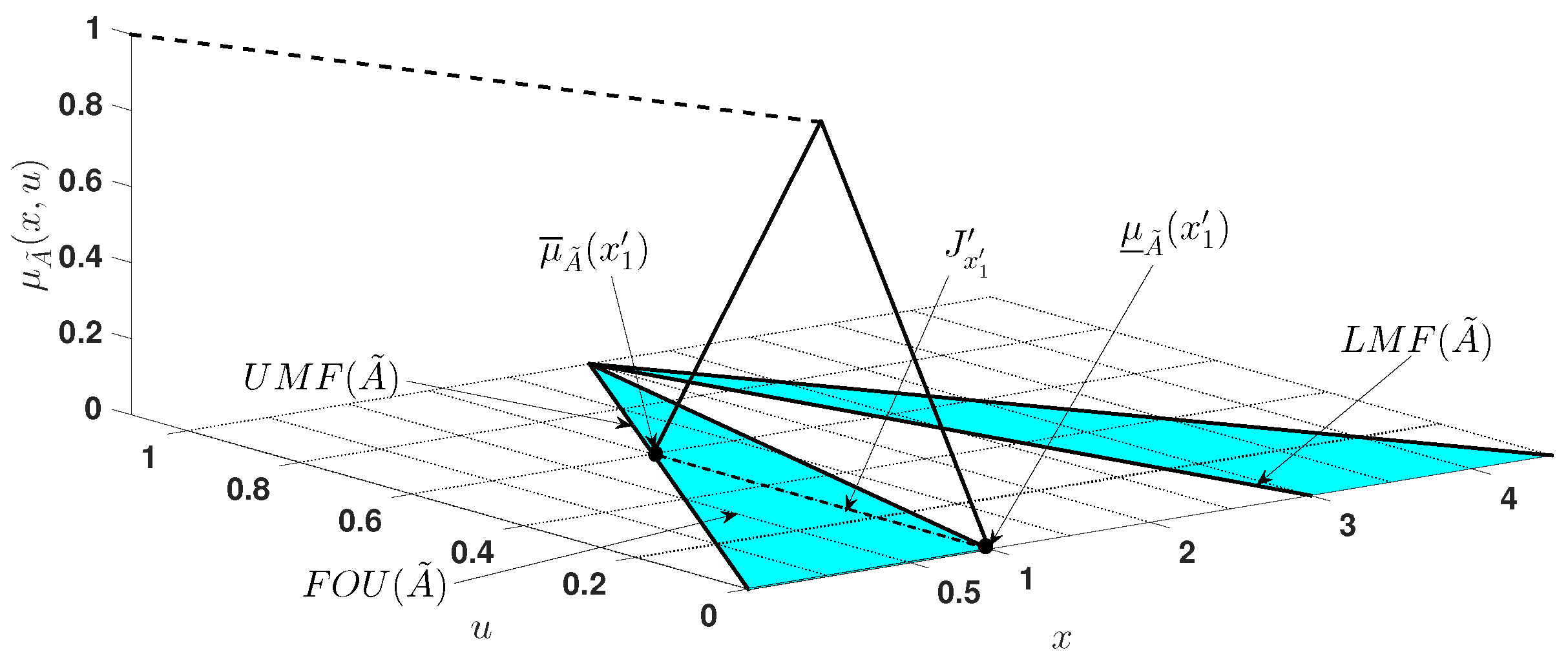
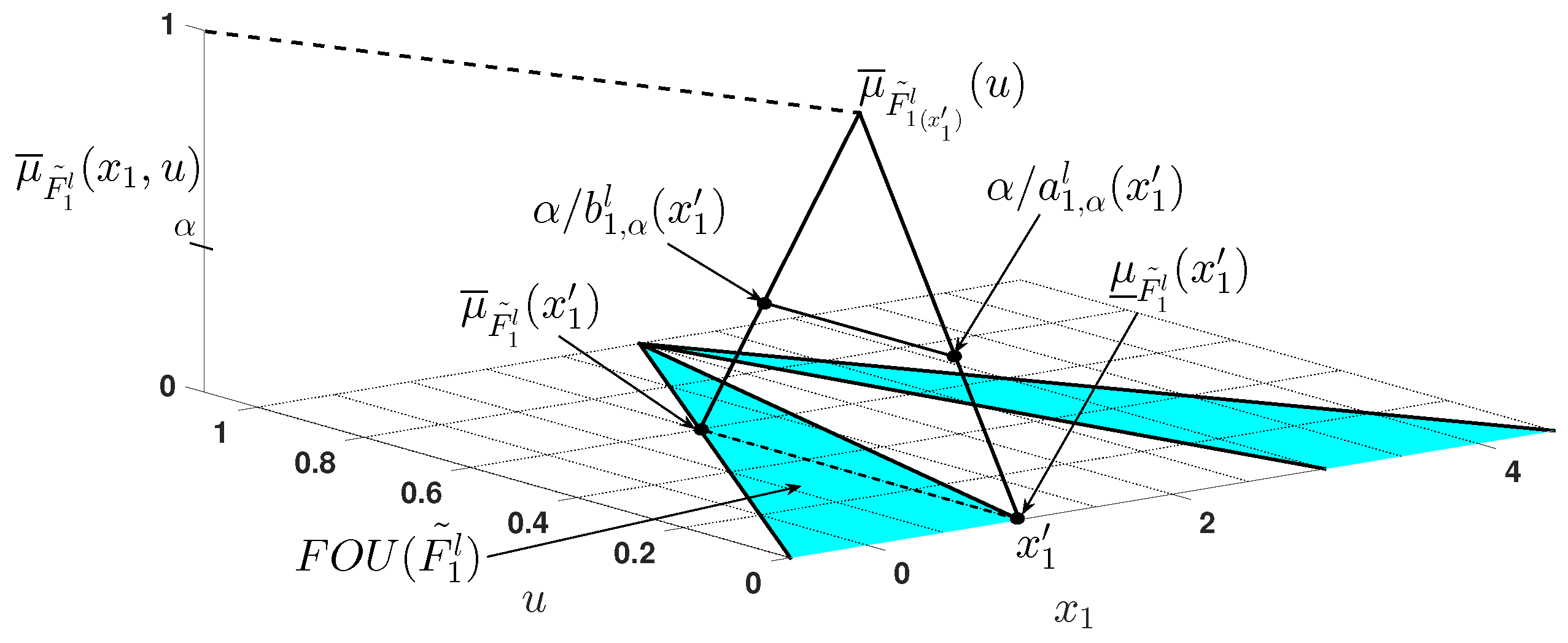
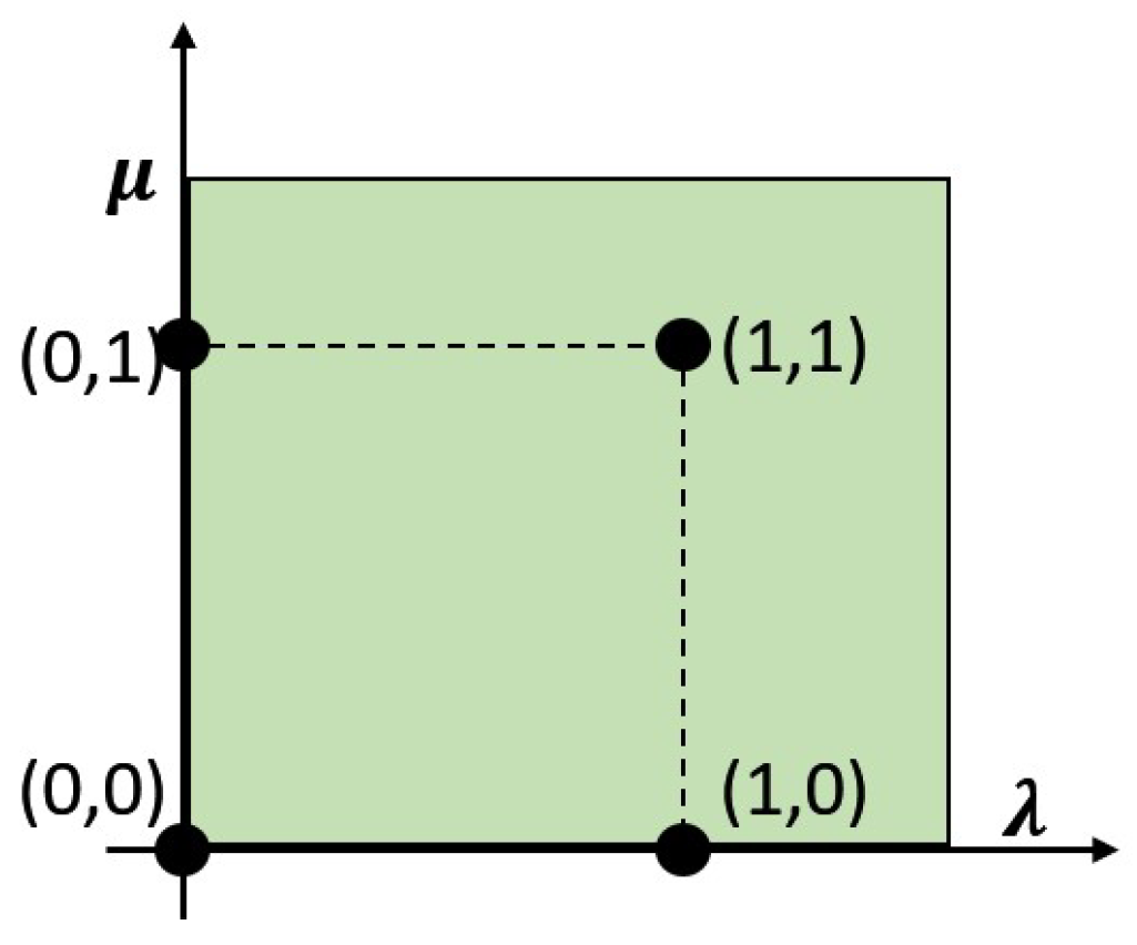
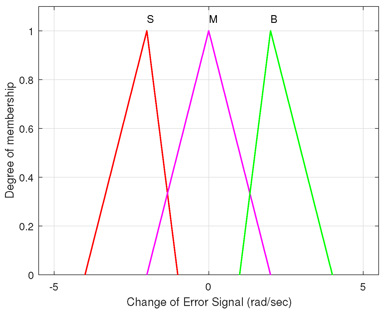
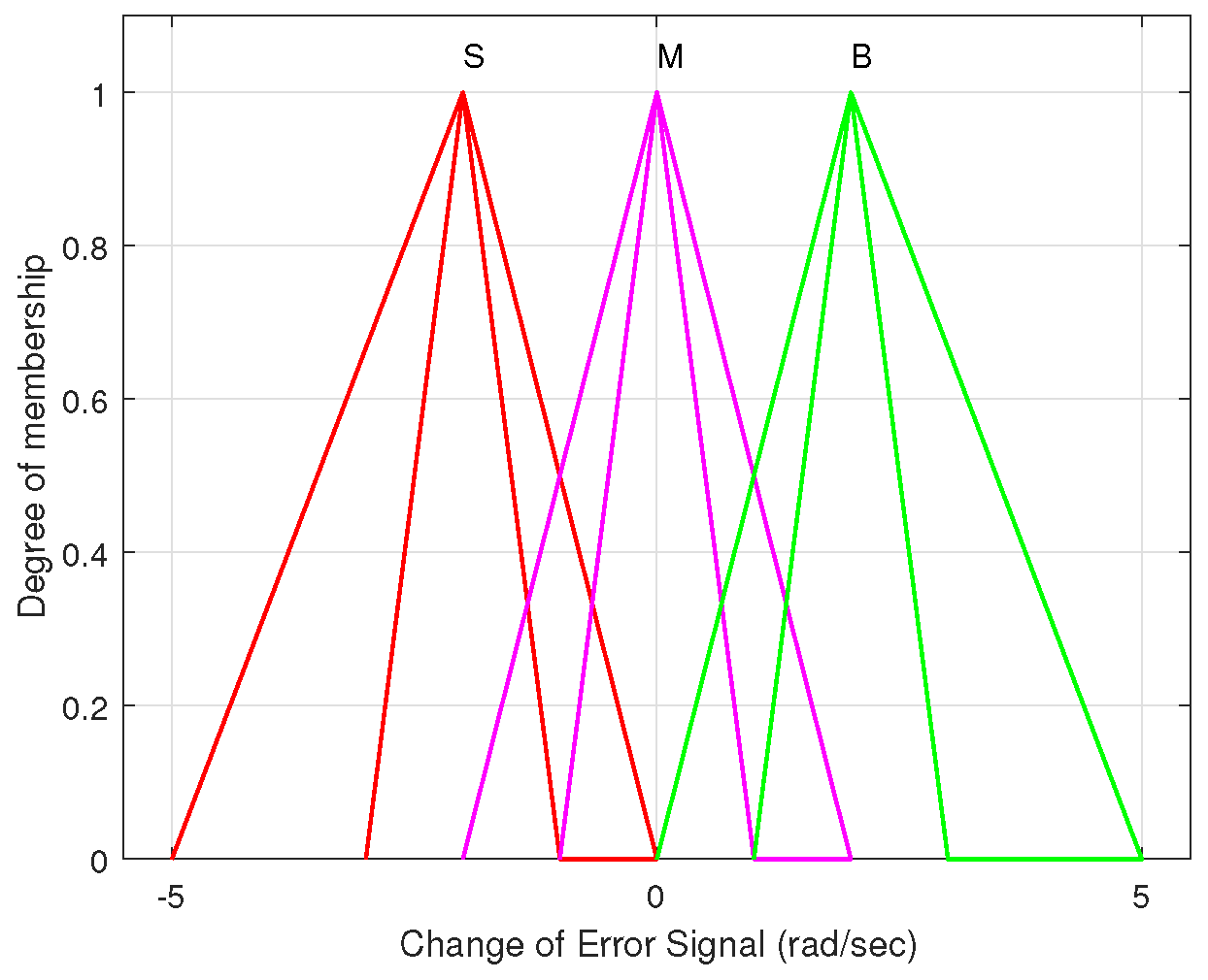
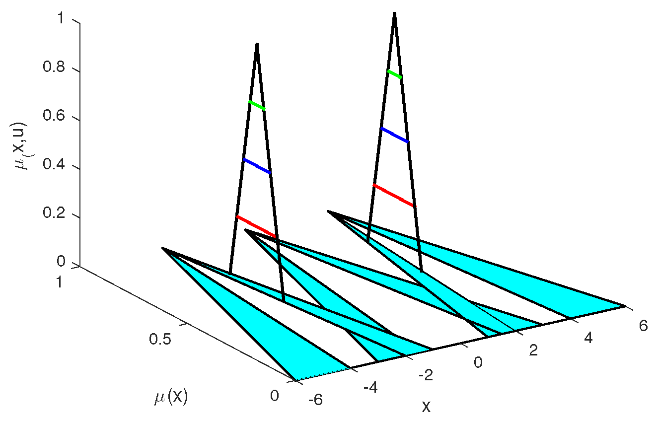
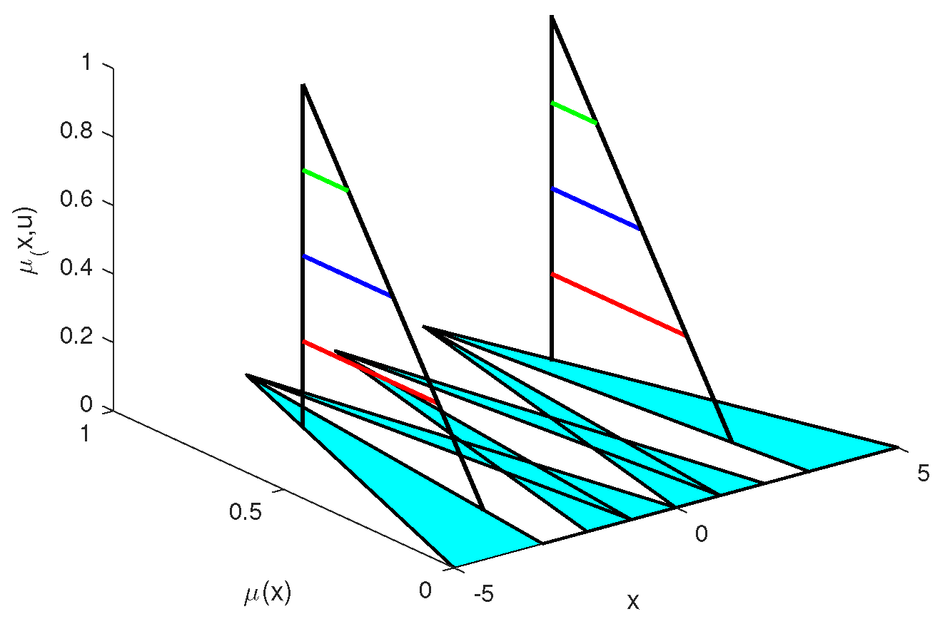
2.1. General Type-2 Fuzzy Sets
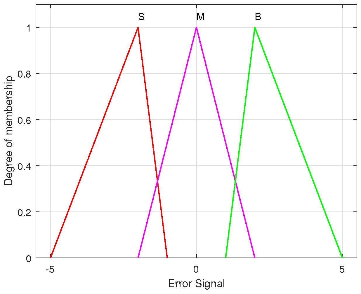
There are several mathematical definitions of a GT2-FLS, and the GT2-FS can be defined as Equation (1) based on [30].
A ˜ ˜ = { ( ( x , u ) , μ A ˜ ( x , u ) ) | x X , u J x [ 0 , 1 ] } ,
where J x is an interval set and as described as Equation (5), x is the partition of the primary MF, and u is the partition of the secondary MF. In this case, Figure 2 shows the various elements of a GT2-FS, whose secondary MF is a triangle function.
As the Figure 2 shows, the footprint of uncertainty ( F O U ) is represented by the blue area and defined as Equation (2). Moreover, the upper membership function (UMF) and the lower membership function (LMF) are associated with the upper and lower boundaries of F O U ( A ˜ ) , and they are denoted as μ ¯ A ˜ ( x ) and μ ̲ A ˜ ( x ) , which are defined as Equations (3) and (4), respectively. Note that in GT2-FS the uncertainty is depicted by a volume, which demonstrates that the GT2-FS is more capable of handling uncertainty.
F O U ( A ˜ ) = x X J x = { ( x , u ) : u J x [ 0 , 1 ] }
μ ¯ A ˜ ( x ) = F O U ( A ˜ ) ¯ x X
μ ̲ A ˜ ( x ) = F O U ( A ˜ ) ̲ x X
Note that J x is an interval set, as follows:
J x = { ( x , u ) : u [ μ ̲ A ˜ , μ ¯ A ˜ ] }

2.2. Rule Base

The rules of a GT2-FLS have two different canonical structures, Zadeh and TSK. The structure of the Zadeh rule are used and introduced in this paper. In the proposed method, the error and the change in error are antecedents, so the specific general type-2 (GT2) Zadeh rule is written as
R l : I F e i s F 1 l ˜ ˜ a n d Δ e i s F 2 l ˜ ˜ , T H E N y i s G l ˜ ˜ , w h e r e l = 1 , M ,
where R l is a specific rule, the F 1 l ˜ ˜ and F 2 l ˜ ˜ are inputs’ MF on rule l, G l ˜ ˜ is outputs’ MF on rule l. Both F ˜ ˜ and G ˜ ˜ are GT2-FS and described as Figure 2.

2.3. Fuzzy Inference Engine

The focus of this subsection is on results just for singleton fuzzification and convex MFs. As illustrated in Figure 3, for each rule, when x 1 = x 1 , only the vertical slice of the rule-antecedent GT2 FS F i l ˜ , F i l ˜ ( x i ) , is activated. It can be denoted by α -cut as Equation (7) [36].
F i l ˜ ( x i ) = μ F i l ˜ ( x i ) ( u ) = sup α [ 0 , 1 ] [ α / [ a α ( x ) , b α ( x ) ] ]
Moreover, for a GT2 Mamdani fuzzy system, the level α firing set, F α l ( x ) , is
F α l ( x ) α / [ f ̲ α l ( x ) , f ¯ α l ( x ) ]
and
f ̲ α l ( x ) T i = 1 p a i , α l ( x i ) f ¯ α l ( x ) T i = 1 p b i , α l ( x i )
Because the GT2-FS’s secondary MF is a triangle function as in Figure 2, we use the vertical-slice representation of its GT2-FSs to reduce computation complexity. So, the formula for the α -cuts of triangle secondary MFs [36]:
a i , α l ( x i ) = μ ̲ F i l ˜ ( x i ) + w [ μ ¯ F i l ˜ ( x i ) μ ̲ F i l ˜ ( x i ) ] α b i , α l ( x i ) = μ ¯ F i l ˜ ( x i ) ( 1 w ) [ μ ¯ F i l ˜ ( x i ) μ ̲ F i l ˜ ( x i ) ] α ,
where w is the position weight and determines the shape of the triangle secondary MFs.

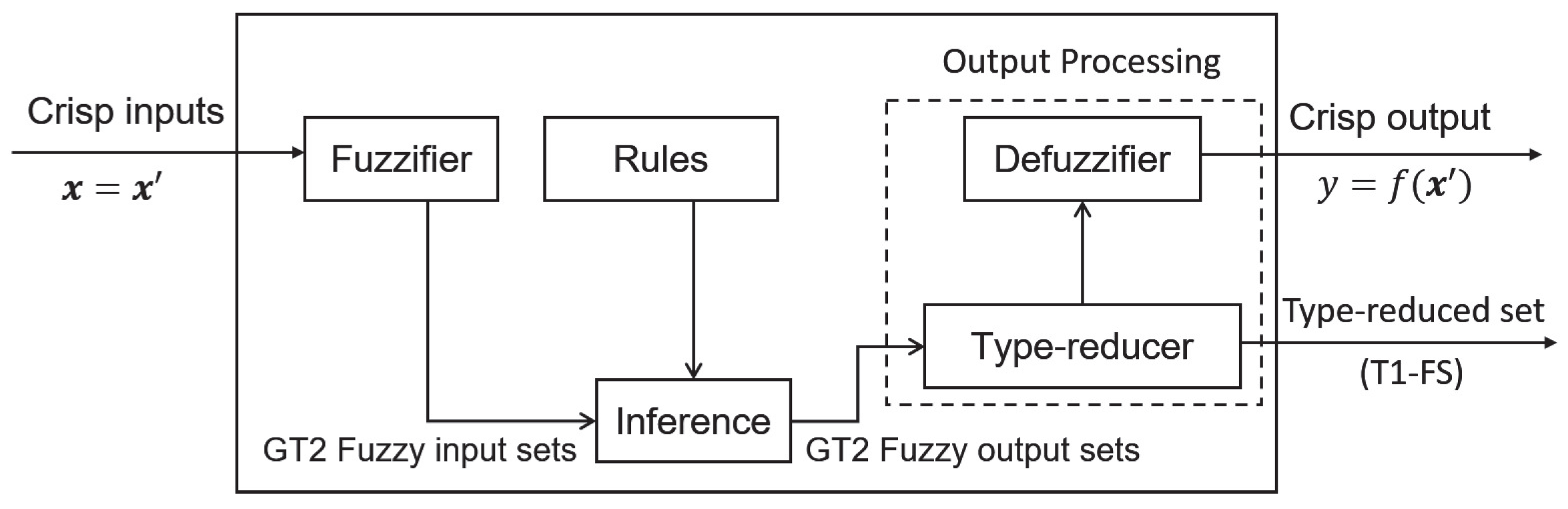
2.4. Type-Reduction and Defuzzification
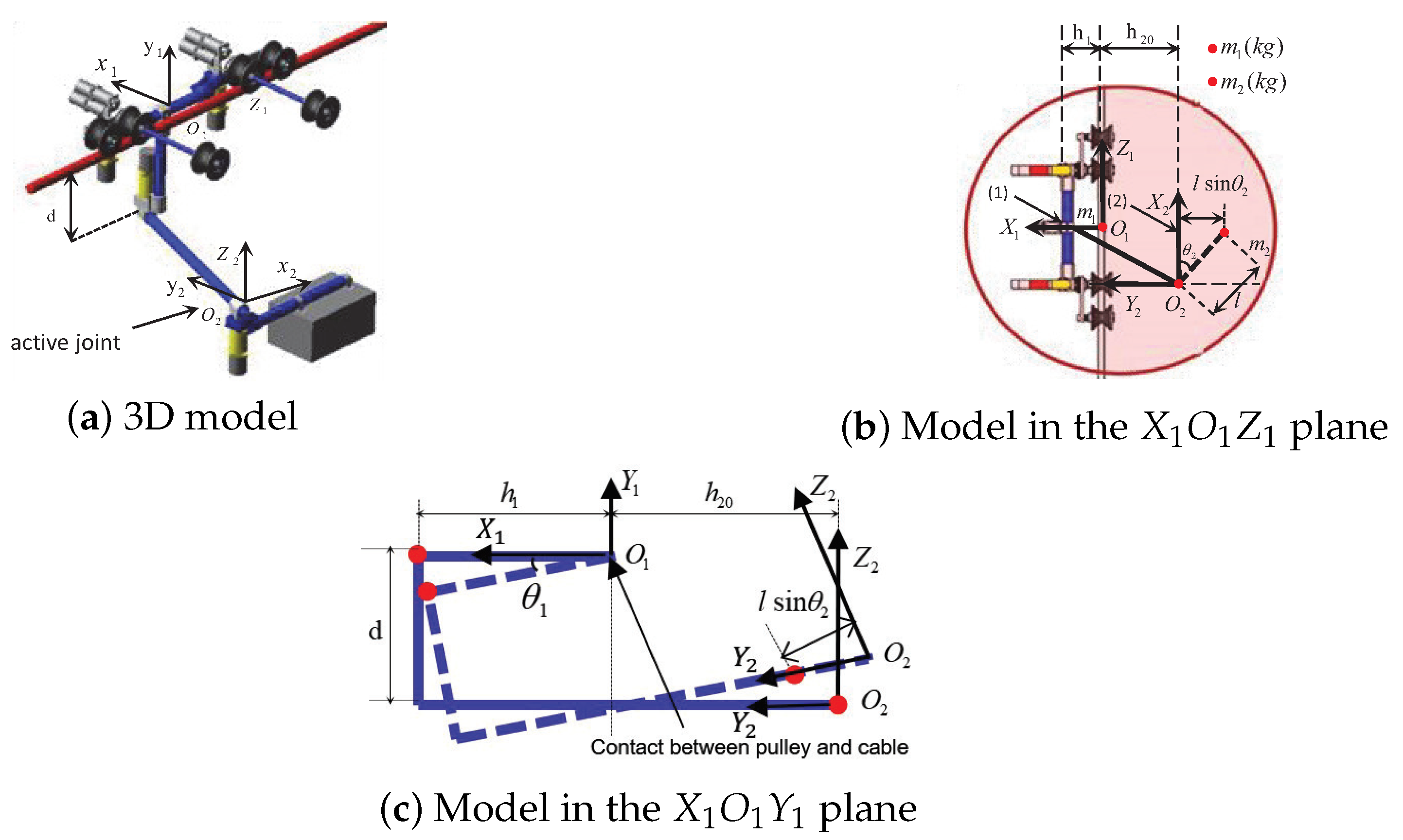
The center-of sets (COS) type-reduction as well as average of end-points defuzzification are performed in this study. To begin, the centroids of the M GT2 Zadeh rule consequent GT2 FSs are computed by Equation (11),
C G ˜ l = sup α [ 0 , 1 ] C G ˜ α l C G ˜ α l = α / [ c l ( G ˜ α l ) , c r ( G ˜ α l ) ] ,
where C G ˜ α l is the centroid of α -plane G ˜ α l a raised to level- α . It should be noted that these centroids do not depend upon x , so these centroids can be computed and stored after the design of the GT2-FLS has been completed [37].
Next, the M C G ˜ α l and the level α firing set F α l ( x ) are used to compute
Y C O S , α ( x ) = α / [ y l , α C O S ( x ) , y r , α C O S ( x ) ] ,
and y l , α C O S ( x ) , y r , α C O S ( x ) can be computed by Equation (13).
y l , α C O S ( x ) = i = 1 L c l ( G ˜ α l ) f ¯ α i ( x ) + i = L + 1 M c l ( G ˜ α l ) f ̲ α i ( x ) i = 1 L f ¯ α i ( x ) + i = L + 1 M f ̲ α i ( x ) y r , α C O S ( x ) = i = 1 R c r ( G ˜ α l ) f ̲ α i ( x ) + i = R + 1 M c r ( G ˜ α l ) f ¯ α i ( x ) i = 1 R f ̲ α i ( x ) + i = R + 1 M f ¯ α i ( x ) ,
where f ̲ α i ( x ) and f ¯ α i ( x ) are end-points of the level α firing interval for the ith rule and computed by Equation (9).
At last, we can conclude that the defuzzified output of the GT2-FLC can be denoted as Equation (14).
Y C O S ( x ) = α [ 0 , 1 ] Y C O S , α ( x ) = α [ 0 , 1 ] α / [ y l , α C O S ( x ) , y r , α C O S ( x ) ]

3. PLI Robot System

The PLI robot system covered in this section is cited from [38]. Figure 4 and Figure 5 show the overall structure and modeling framework of the PLI robot, respectively. It should note that there is a counter-weight to balance the PLI robot system. This self-balancing mechanism balances the robot by adjusting the center of gravity of the counter-weight.

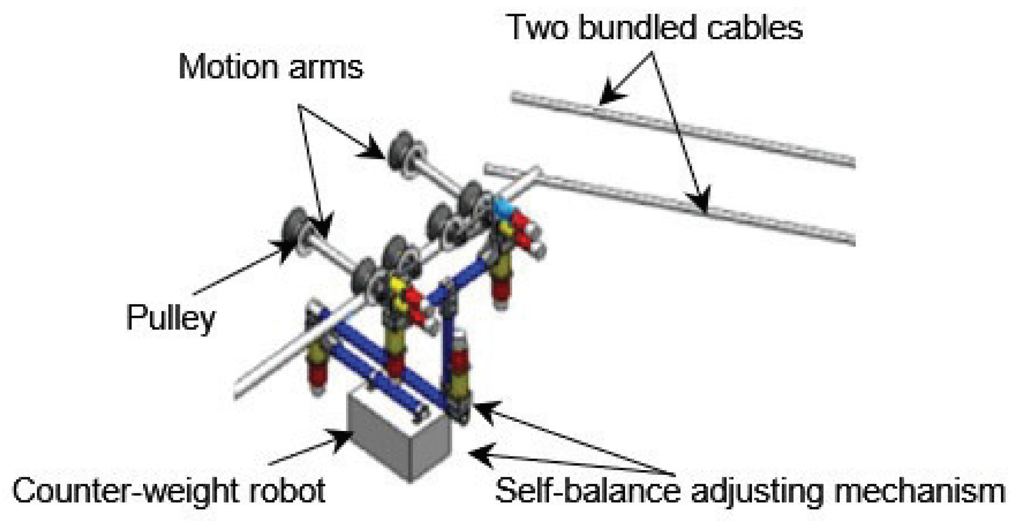
Mathematical Model of PLI Robot System

Firstly, as shown in Figure 4 and Figure 5, θ 1 ( t ) is the tilt angle between the robot body and the X 1 axis, and θ 2 ( t ) is the angle at which the weight adjusts the center of mass (COM) of the robot to achieve equilibrium rotation. h 1 is the vertical distance between the COM of the PLI robot and the cable, and h 20 is the distance from the COM of the counter-weight box to the Y 1 O 1 Z 1 plane at θ 1 = 0 . u 2 ( t ) is the torque produced by the active joint attached to the weight block. τ 1 ( t ) is the external disturbance.
Secondly, the dynamic model of PLI robot system is established by the Euler-Lagrange equation, and the Lagrangian is given as Equation (15).
L = K P ,
u i = d d t L θ i ˙ L θ i i = 1 , , m
where u i is the torque acting on the ith generalized coordinate, K is the kinetic energy of the PLI robot, P is the potential energy of the PLI robot. The K and P can be denoted as Equations (17) and (18).
K = m 1 h 1 2 θ 1 2 ˙ 2 + m 2 l 2 θ 2 2 ˙ 2 + m 2 [ d 2 + ( h 20 + l s i n θ 2 ) ] θ 1 2 ˙ 2
P = m 1 g h 1 s i n θ 1 + m 2 g [ h c o s θ 1 ( h 20 + l s i n θ 2 ) s i n θ 1 ] ,
where g is the acceleration of gravity. From Table 1, we can get
m 1 h 1 = m 2 h 20 ,
from Equations (18) and (19), P can be rewritten as Equation (20).
P = m 2 g ( d cos θ 1 + l sin θ 2 sin θ 1 ) .
Substituting Equations (17) and (20) into Equation (16), and then substituting Equation (16) into Equation (15) to derive the dynamic equations of the PLI robot system. Therefore, the dynamic equations are as follows:
τ 1 = [ m 1 h 1 2 + m 2 ( d 2 + ( h 20 + l sin θ 2 ) 2 ) θ 1 ¨ ] + 2 m 2 l ( h 20 + l sin θ 2 ) ( cos θ 2 ) θ 1 ˙ ϑ 2 ˙ + m 2 g d sin θ 1 + m 2 g l sin θ 2 cos θ 1 u 2 = m 2 l 2 θ 2 ¨ m 2 l ( h 20 + l s i n θ 2 ) ( c o s θ 2 ) θ 1 2 ˙ + m 2 g l c o s θ 2 s i n θ 1
To better describe the dynamic process, the state variable vector is defined as follows:
x = [ x 1 x 2 x 3 x 4 ] T = [ θ 1 θ 1 ˙ θ 2 θ 2 ˙ ] T .
The parameters of the PLI robot are shown in Table 1. Therefore, the state space model of the PLI robot are as follows:
x 1 ˙ = x 2 x 2 ˙ = τ 1 2 m 2 l ( h 20 + l sin x 3 ) ( cos x 3 ) x 2 x 4 [ m 1 h 1 2 + m 2 ( d 2 + ( h 20 + l sin x 3 ) 2 ) ] m 2 g d sin x 1 + m 2 g l sin x 3 cos x 1 [ m 1 h 1 2 + m 2 ( d 2 + ( h 20 + l sin x 3 ) 2 ) ] x 3 ˙ = x 4 x 4 ˙ = u 2 + m 2 l ( h 20 + l sin x 3 ) ( cos x 3 x 2 2 ) m 2 l 2 m 2 g l cos x 3 sin x 1 m 2 l 2

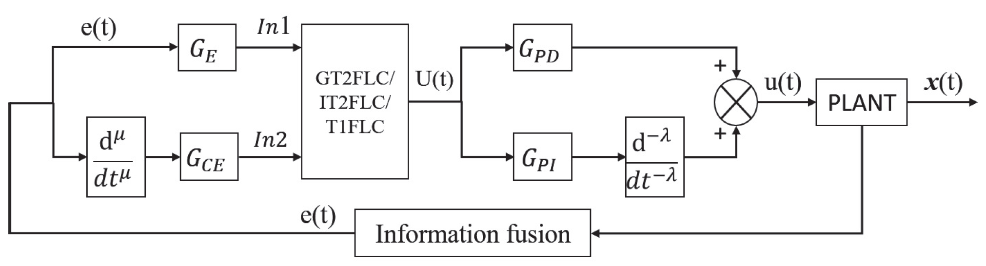
4. Design of GT2FO-FPID Controller

The description of design and implementation of the GT2FO-FPID controller is presented in this section. The GT2-FLS is used to design the GT2FO-FPID controller in the MATLAB environment.

4.1. Approximations of Fractional Order Operation

In the development of fractional calculus theory, the definition of fractional calculus of many functions appears, such as the Cauchy integral formula directly extended by integer calculus, Grünwald-Letnikov (GL), Riemann-Liouville (RL) and Capotu definitions etc. Cauchy, GL and RL integral formulas are directly extended from integral of integer order. Among them, GL is the most direct numerical method to solve fractional calculus, because its coefficients w j ( α ) in Equation (26) can be calculated by simple recursive formulas (Equation (27)). Cauchy and RL formulas are more complicated, which will increase the computational complexity of the controller. Therefore, in this study, the GL definition is used to define and calculate fractional calculus, as shown in Equation (24).
a D t α f ( t ) = lim h 0 1 h α j = 0 [ ( t a ) / h ] ( 1 ) j α j f ( t j h ) ,
where α j is the binomial coefficient. It should note that the a D t α has three circumstance as described as Equation (25).
a D t α = d α d t α R ( α ) > 0 1 a t ( d τ ) α R ( α ) < 0 ,
where a is initial conditions and α is fractional order operator, α R . R stands for Real.
In this study, the GL definition is used to approximate the fractional calculus, and given by Equations (26) and (27).
a D t α f ( t ) = lim h 0 1 h α j = 0 [ ( t a ) / h ] ( 1 ) j α j f ( t j h ) 1 h α j = 0 [ ( t a ) / h ] w j ( α ) f ( t j h ) ,
w 0 ( α ) = 1 , w j ( α ) = ( 1 α + 1 j ) w j 1 ( α ) , j = 1 , 2 ,
where w j ( α ) = ( 1 ) j α j is the polynomial coefficient of the function ( 1 z ) α , the coefficient can be directly obtained by the following recursive formula. Assuming that the step size h is small enough, the approximation of the numerical differential of the function can be directly obtained by the formula Equation (27), and it can be proved that the precision of the formula is o ( h ) [39].

4.2. Structure of PI λ D μ Controller

The PI λ D μ controller output u ( t ) can be depicted by Equation (28).
u ( t ) = K p e ( t ) + K d d μ d t μ ( e ( t ) ) + K i d λ d t λ ( e ( t ) ) , μ , λ > 0 ,
where K p , K d , K i are proportional gain, derivative gain, integral gain, respectively. μ and λ are fractional order derivative value and fractional order integral value, respectively.
As illustrated in Figure 6, there are four cases for the common PID controllers: (1) The conventional PD controller when ( μ , λ ) = ( 0 , 1 ) ; (2) The conventional PI controller when ( μ , λ ) = ( 1 , 0 ) ; (3) The conventional PID controller when ( μ , λ ) = ( 1 , 1 ) ; (4) A proportional gain can be realized when ( μ , λ ) = ( 0 , 0 ) . It should note that all these common types of PID controllers are the special cases of the PI λ D μ controller. Moreover, it can be intuitively seen that the PI λ D μ controller is a generalization of the integer order PID controller, and the PI λ D μ controller has two degrees of freedom more than the integer order PID controller, so its flexibility is better.

4.3. Structure of GT2FO-FPID Controller

In this section, the structure and design strategy of the proposed controller are introduced. The overall frame of the GT2FO-FPID controller is shown in the Figure 7. As illustrated in Figure 7, there are six structural parameters, and we optimize the parameters by the GA algorithm.
Firstly, it can be observed that there is a module for information fusion from the Figure 7. Since the controlled object is an under-actuated system, it is necessary to obtain all the information of the system to achieve better control. However, when all four state information is input as the system, it is inevitable to encounter a rule explosion problem. Therefore, the information fusion involved in [40] is used to solve the problem.
Secondly, the specific process of information fusion is as follows [40]:
(a) Construct the state feedback gain matrix. Using the quadratic optimal control theory, the state feedback matrix K is calculated by selecting the appropriate weighting matrix Q, R to satisfy the condition that the quadratic performance index J of the system model is minimized.
J = 0 [ x T ( t ) Q x ( t ) + u 2 T ( t ) R u 2 ( t ) ] d t
K = [ K x 1 K x 3 K x 2 K x 4 ] ,
where T represents the transposition of the matrix, K x 1 , K x 2 , K x 3 , K x 3 are the feedback coefficients of x 1 , x 2 , x 3 , x 4 , respectively. The controller can be adjusted to obtain the desired response by changing the non-zero elements in the Q matrix, the greater the value of the non-zero elements indicating the more significant the effect of the corresponding state variable on the system.
(b) Construct the fusion function F x using the state feedback gain matrix. In view of the fact that the four state information is directly used as the input of the controller, the problem of rule explosion occurs, so the information state fusion is first reduced by information fusion. Considering that the main control variable is x 1 , x 1 and x 2 are selected as the control principals of the system, x 3 and x 4 are used as control sub-elements of the system, and according to the correlation and the fusion with the principal elements, they are merged into the two control principals.
Therefore, the process of the fusion function and the input-output equation are as follows:
u 2 = K · x = K x 1 · x 1 + K x 2 · x 2 + K x 3 · x 3 + K x 4 · x 4 = K x 1 [ x 1 + K x 3 K x 1 · x 3 ] + K x 2 [ x 2 + K x 4 K x 2 · x 4 ] = K x 1 · x ˜ 1 + K x 2 · x ˜ 2 ,
and then the fusion function F x is as follows:
F x = 1 0 K x 3 K x 1 0 0 1 0 K x 4 K x 2 .
(c) The four state variables fusion into two variables:
e e c = F x × x T ,
It can be observed from the above equation that information fusion not only achieves system dimensionality reduction but also contains all state information of the system. It also should note that only the e is used when controlling the PLI robot system.
Thirdly, as Figure 7 shows, e ( t ) and e c ( t ) are the inputs of the controllers. Each input is divided into three groups of linguistic variables, i.e., small (S), middle (M), big (B) as Figure 8, Figure 9, Figure 10, Figure 11, Figure 12 and Figure 13. The input membership functions of type-1, interval type-2, and general type-2 are illustrated by Figure 8, Figure 9, Figure 10, Figure 11, Figure 12 and Figure 13, respectively. It should note that the GT2-FSs’ secondary MFs are triangle functions. Furthermore, there are five α -planes ( α = 0, 0.25, 0.5, 0.75, 1) used to reduce the computational complexity of GT2-FSs. The rule base is based on the expert’s knowledge and experience. We mainly design fuzzy rules based on years of PID control experience. For example, at the beginning of control, the controller needs to generate a large control signal to quickly start the control process. In order to generate a large control signal, a large proportional gain k p , a large integral gain k i and a small differential gain k d are required. When approaching the equilibrium point, a smaller proportional gain k p , a smaller integral gain k i and a larger differential gain k d are needed to avoid deviation from the equilibrium state to construct a smaller control signal. Therefore, the fuzzy rules are generated as shown in Table 2.
Remark 1.
Both the fractional order PID and the GT2-FLC are controllers with more degrees of freedom, which means that selecting the appropriate parameters enables the controller to achieve better control performance. Therefore, we combine these two controllers in anticipation of an improvement in control results.
Finally, the GT2FO-FPID controller is applied to the PLI robot system to achieve the balance. The corresponding numerical simulation will be given in next section.

5. Simulation

In this section, the proposed controller’s performance and robustness are compared to other controllers; IT2FO-FPID, T1FO-PID, and FOPID on the PLI robot system. Furthermore, the three kinds of evaluation functions (ISE, IAE and ITAE) are used to assess the control performance of controllers and are defined as:
I S E = 0 e ( t ) 2 d t
I A E = 0 | e ( t ) | d t
I T A E = 0 | e ( t ) | t d t
The matrix Q, R and K 1 are as follows:
Q = d i a g [ 250 , 150 , 150 , 50 ] , R = 10 ,
K = [ 9.4663 6.773928 28.2025 7.8361 ] ,
according to available state feedback matrix K 1 , F x is
F x = 1 0 18.7362 0 0 1 0 1.0622 .
Therefore, the four state variables fusion into a e and e c :
e e c = F x × x 1 x 2 x 3 x 4 .
Moreover, the selection of the objective functions of the GA is as follows:
O b j _ f 1 = 0 | e 1 ( t ) | t d t O b j _ f 2 = 0 | e 2 ( t ) | t d t O b j _ f = ω 1 O b j _ f 1 + ω 2 O b j _ f 2 ,
where e 1 ( t ) is the difference between state variable x 1 and its expected value, e 2 ( t ) is the difference between state variable x 3 and its expected value. The ω 1 and ω 2 are the weights of the corresponding functions, respectively. In this study, both ω 1 and ω 2 are equal to 0.5. In order to obtain the optimal parameters within the range, we took the objective function (Equation (41)) as the evaluation function and iterated through GA algorithm for several times until the value of the evaluation function converges. The main optimization parameters include: G E , G C E , G P D , G P I , λ and μ . The optimal parameters for GT2FO-FPID, IT2FO-FPID, T1FO-FPID, FOPID controllers are shown in Table 3.
The original position is x = [ 0.3 0 0.3145 0 ] T and the task of control is to return the PIL robot to its balance position x = [ 0 0 0 0 ] T through the self-balancing mechanism. To comprehensively compare the performance of several controllers, there are four simulation tasks performed the PLI robot system.

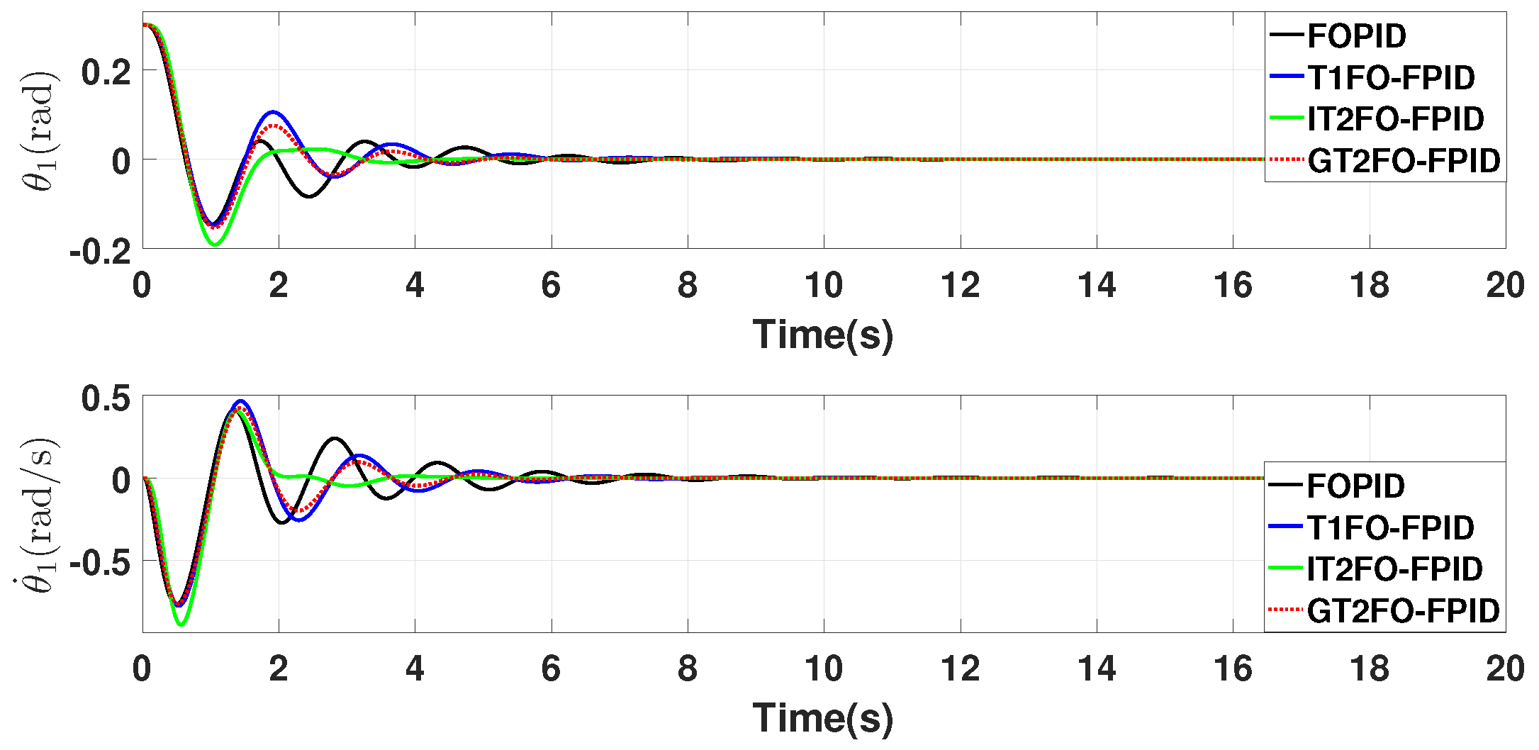
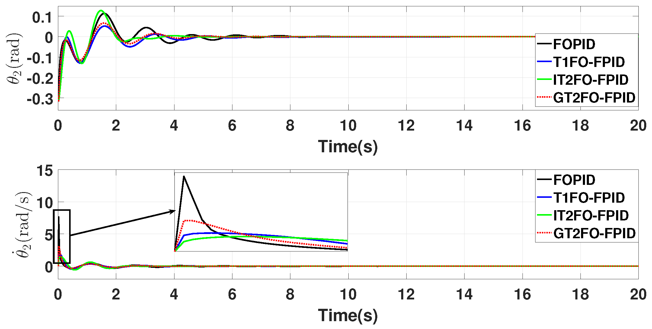
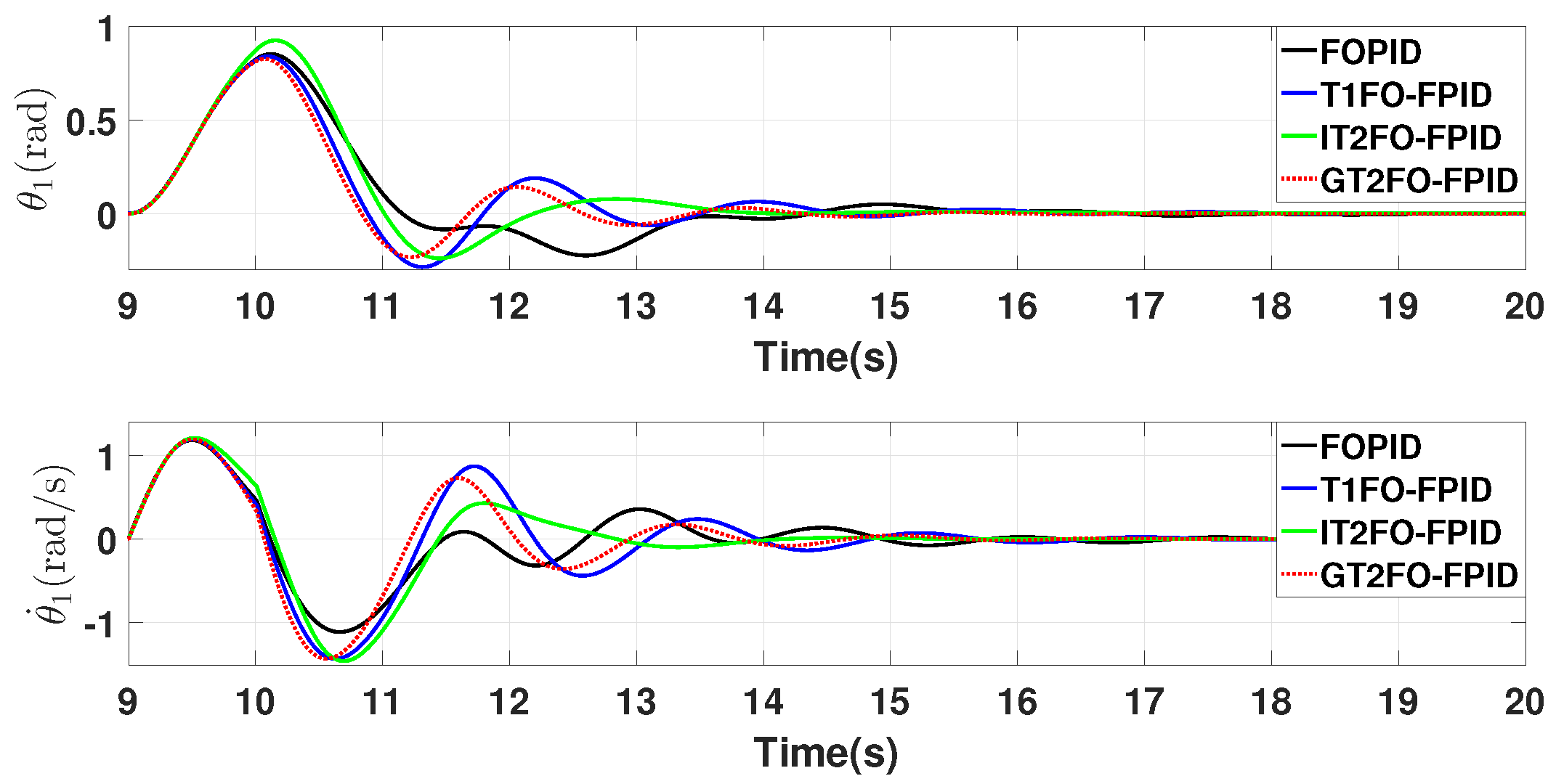
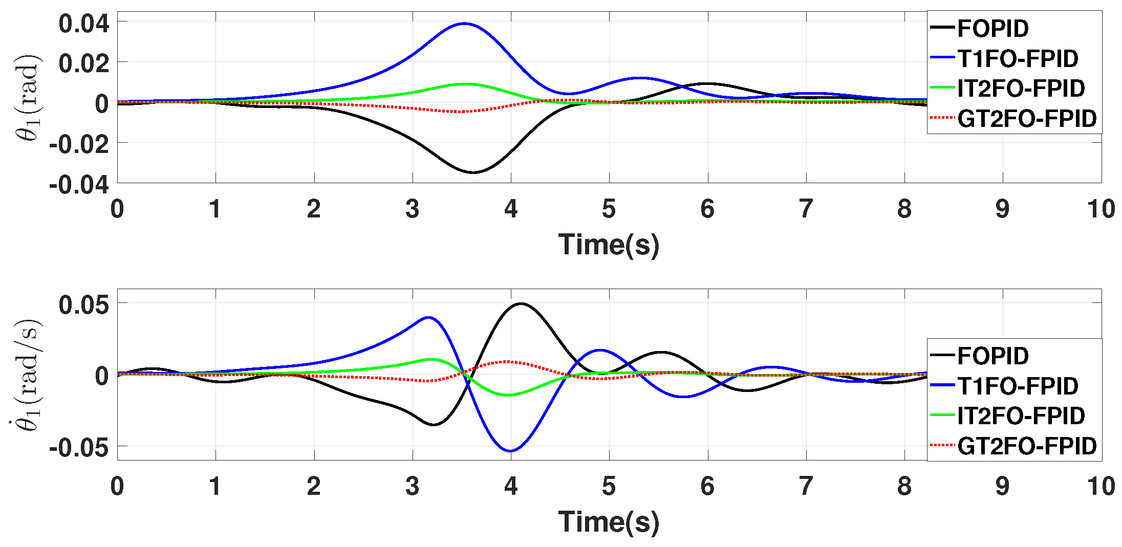
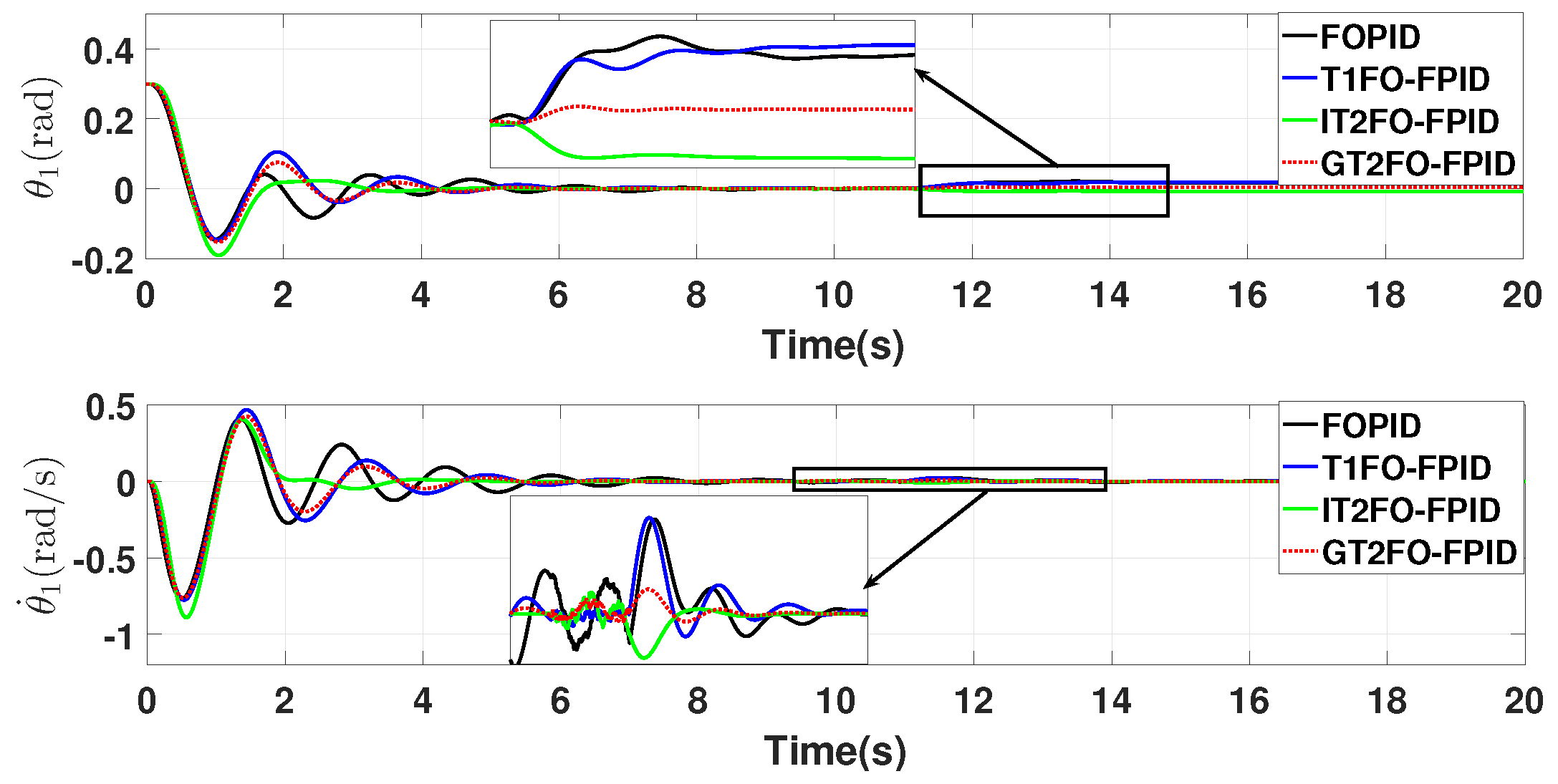
5.1. Case 1: Normal Case

In this case, we assumed that the external interference τ 1 = 0 N · m, and compared the performance of these several controllers. It can be observed from Figure 14 and Figure 15 and Table 4 that the overshoots of GT2FO-FPID and IT2FO-FPID controllers were smaller and the settle times were shorter than other controllers.

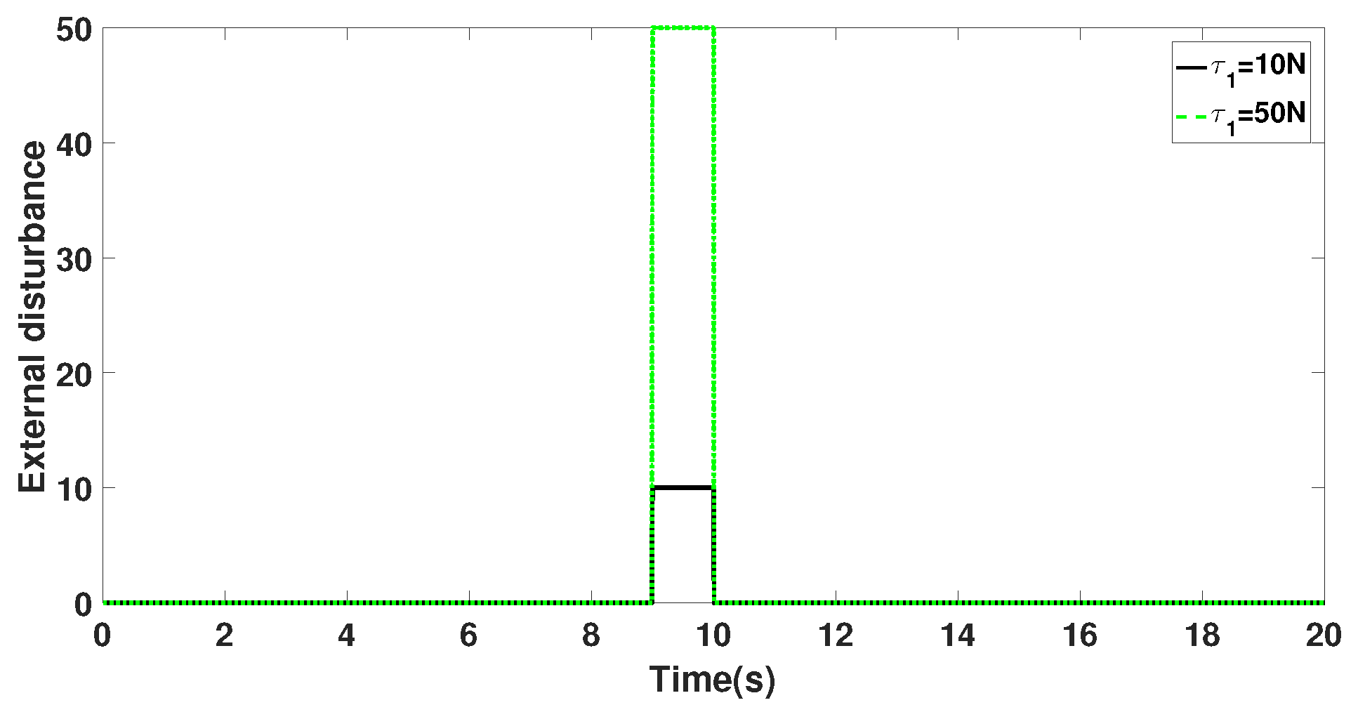
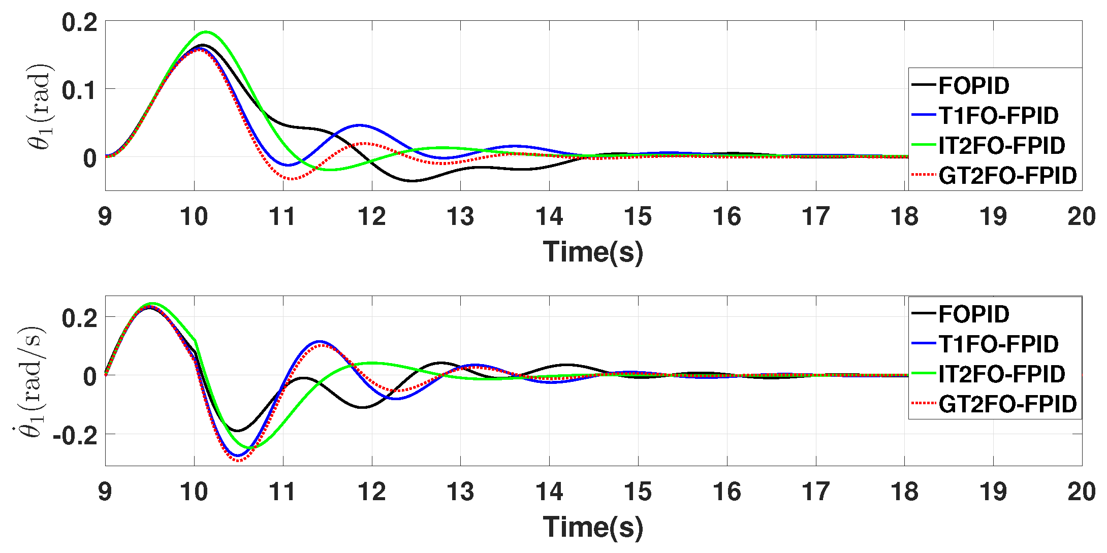
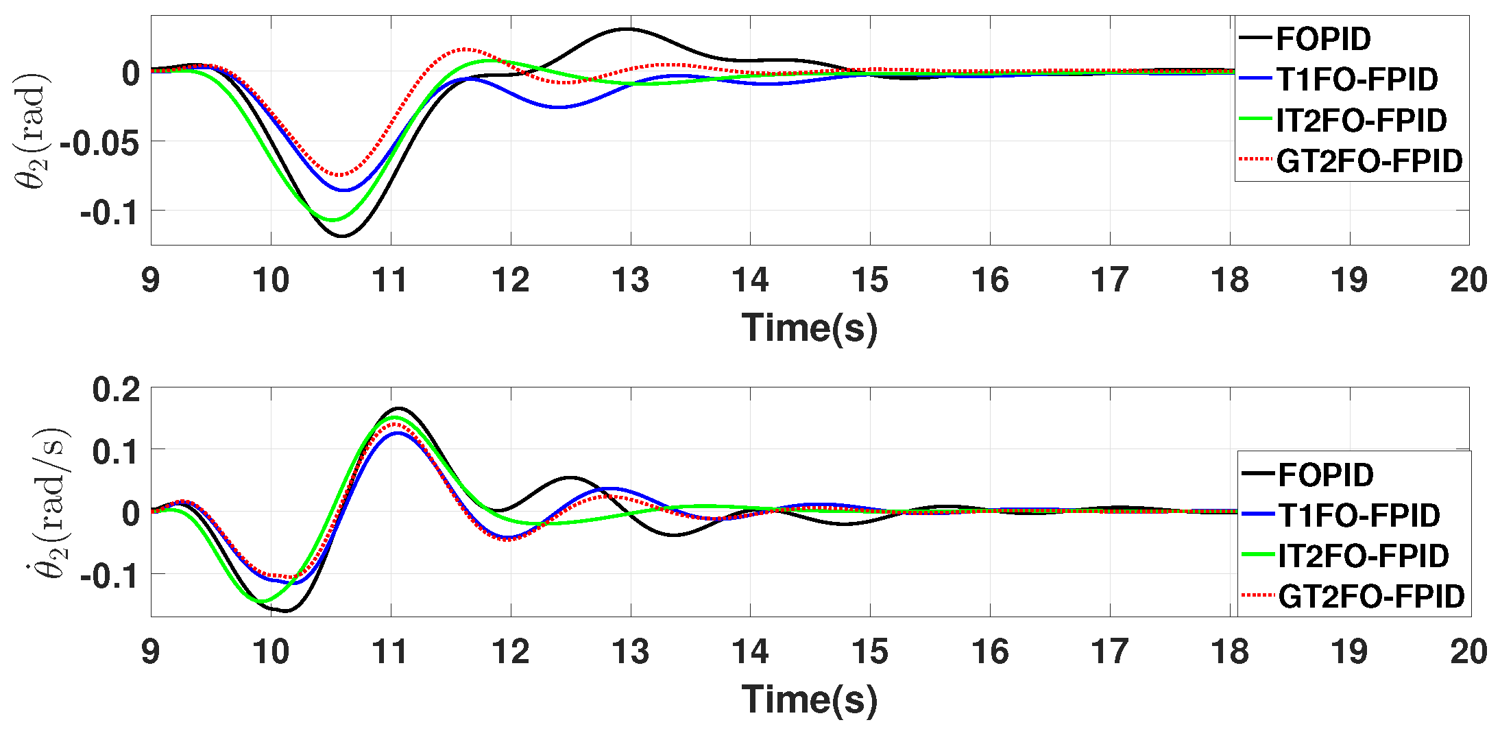
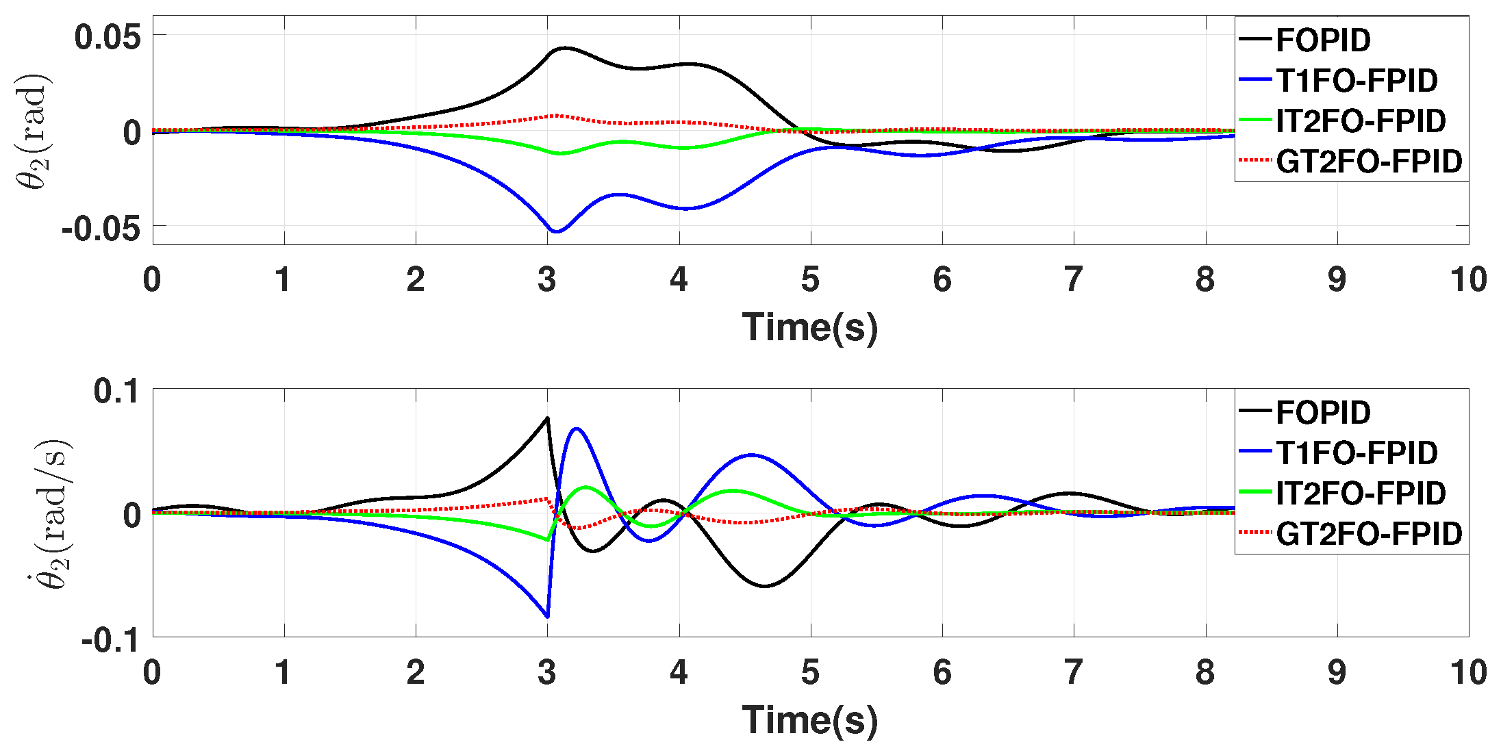
5.2. Case 2: External Disturbance

In this case, we added two external disturbances as Figure 16 ( τ 1 = 10 N/50 N). As shown in Figure 17, Figure 18, Figure 19 and Figure 20, with the increase of external interference, the GT2FO-FPID always maintained the best performance, including smaller amplitude swing after interference and faster return to the balance position after interference disappeared. It can be observed from Table 5 and Table 6 that the parameters of the GT2FO-FPID controller were the best.

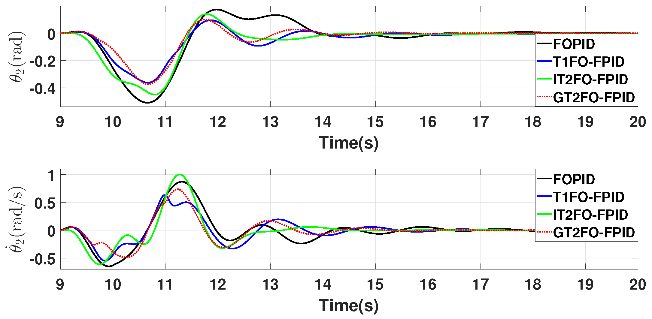
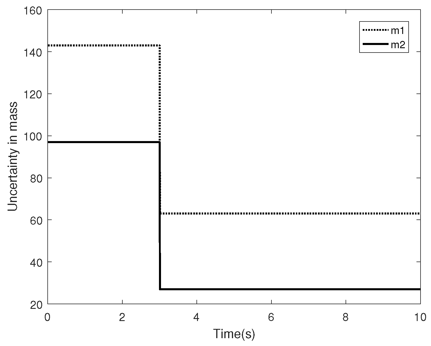
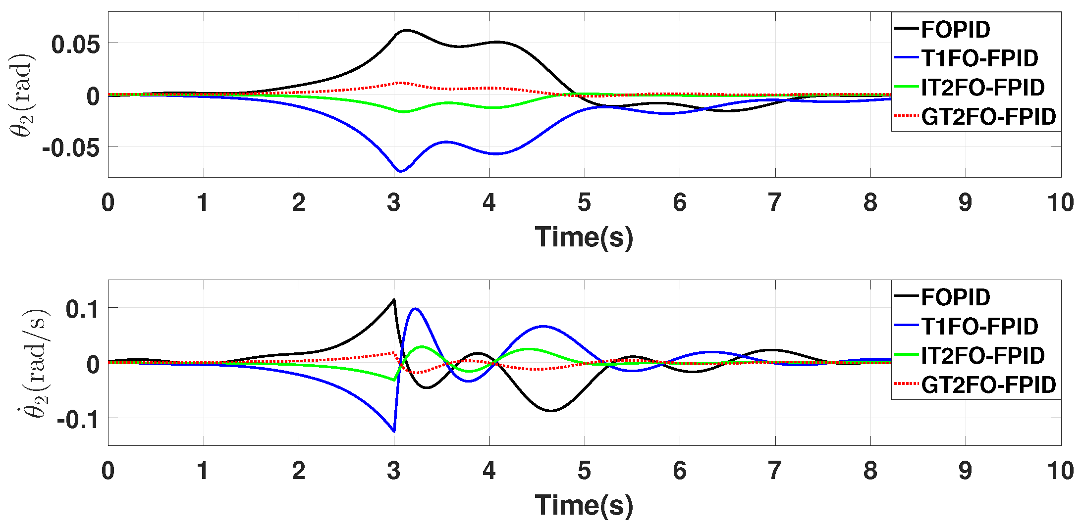
5.3. Case 3: Uncertainty in Mass

To more fully verify the robustness of the proposed controller, a simulation of parameter perturbation was performed. In this case, we put all the controllers in equilibrium and continued for one second before performing the simulation of mass parameter perturbation. Figure 21 illustrates the step change in mass ( Δ m 1 = 80 kg, Δ m 2 = 70 kg). As shown in the Figure 22 and Figure 23 and Table 7, FOPID and T1FO-FPID controllers had large fluctuations after adding square wave interference, and the IT2FO-FPID controller fluctuation was small, while the GT2FO-FPID controller showed the strongest robustness. Furthermore, we increased the variation of mass ( Δ m 1 = 90 kg, Δ m 2 = 80 kg). It can be observed from Figure 24 and Figure 25 and Table 8 that the GT2FO-FPID controller still maintained its control superiority. In a word, the GT2FO-FPID controller exhibited excellent robustness and showed superiority in real applications.

5.4. Case 4: Random Disturbance

Figure 26 and Figure 27 are the outputs of the PLI robot system in the face of random signal interference ( τ 1 = r a n d s ( 1 ) ). According to the system response diagram and Table 9, we can draw the conclusion that the controller proposed in this paper could still maintain the best control performance in the face of random interference.

6. Conclusion and Future Work

6.1. Conclusions

This paper presents a controller combining GT2-FLC with FOPID controller. We are committed to using the advantages of GT2-FLC controller to overcome various uncertainties and the multi-degree of freedom of FOPID controller to improve the performance of the controller. In order to fully verify the proposed controller, we carried out simulation under various interference conditions. In the face of external square wave interference, it can be observed that the GT2FO-FPID controller can still maintain its superiority when the interference signal increases from 10 N to 50 N. In the case of internal parameter perturbation, the GT2FO-FPID controller has almost no fluctuation. In the face of random interference, the performance of the IT2FO-FPID controller and T1FO-FPID controller is not ideal, only the GT2FO-FPID controller can still return to the equilibrium position quickly and accurately. Through this series of numerical simulation, we can conclude that the proposed controller has the best anti-interference ability, especially in the case of internal parameter perturbation. Therefore, we can believe that in real life, the controller proposed in this paper can better achieve the balance control of PLI robot, even if there are a variety of uncertainties.

6.2. Future Work

In future work, we hope to implement the proposed method in real world, verify its effectiveness, and adjust it according to the actual situation. Moreover, when designing input membership functions and rules, we first design through experience, and then slowly adjust, lacking wide applicability. Therefore, in future work, we hope that the system can learn input membership functions and rules and optimize it to improve the adaptability and intelligence of the system in the real world.

Author Contributions

T.Z. proposed the conceptualization and conducted supervision and data management; Y.C. mainly carried out the following work: investigation, methodology, software and writing—review and editing; S.D. did project administration and supervision; validation and writing—original draft were completed by H.W.; X.Z. acquired the funding. All authors have read and agreed to the published version of the manuscript.

Funding

This work is supported by the State gird headquarters Science and Technology Projects of China (Grant No. 5500-201916260A-0-0-00).

Conflicts of Interest

The authors declare no conflicts of interest. The sponsor does not play any role in the work.

References

  1. Caponetto, R. Fractional Order Systems: Modeling and Control Applications; World Scientific: Singapore, 2010; Volume 72. [Google Scholar]
  2. Kumar, A.; Kumar, V. A novel interval type-2 fractional order fuzzy PID controller: Design, performance evaluation, and its optimal time domain tuning. ISA Trans. 2017, 68, 251–275. [Google Scholar] [CrossRef] [PubMed]
  3. Podlubny, I. Fractional-order systems and PλDμ controllers. IEEE Trans. Autom. Control 1999, 44, 208–214. [Google Scholar] [CrossRef]
  4. Monje, C.A.; Vinagre, B.M.; Feliu, V.; Chen, Y. Tuning and auto-tuning of fractional order controllers for industry applications. Control Eng. Pract. 2008, 16, 798–812. [Google Scholar] [CrossRef] [Green Version]
  5. Cao, J.Y.; Liang, J.; Cao, B.G. Optimization of fractional order PID controllers based on genetic algorithms. In Proceedings of the IEEE International Conference on Machine Learning and Cybernetics, Guangzhou, China, 18–21 August 2005; Volume 9, pp. 5686–5689. [Google Scholar]
  6. Padula, F.; Visioli, A. Tuning rules for optimal PID and fractional-order PID controllers. J. Process Control 2011, 21, 69–81. [Google Scholar] [CrossRef]
  7. Bohannan, G.W. Analog fractional order controller in temperature and motor control applications. J. Vib. Control 2008, 14, 1487–1498. [Google Scholar] [CrossRef]
  8. Zamani, M.; Karimi-Ghartemani, M.; Sadati, N.; Parniani, M. Design of a fractional order PID controller for an AVR using particle swarm optimization. Control Eng. Pract. 2009, 17, 1380–1387. [Google Scholar] [CrossRef]
  9. Bouarroudj, N. A hybrid fuzzy fractional order PID sliding-mode controller design using PSO algorithm for interconnected nonlinear systems. J. Control Eng. Appl. Inform. 2015, 17, 41–51. [Google Scholar]
  10. Sharma, R.; Rana, K.P.S.; Kumar, V. Performance analysis of fractional order fuzzy PID controllers applied to a robotic manipulator. Expert Syst. Appl. 2014, 41, 4274–4289. [Google Scholar] [CrossRef]
  11. Bhimte, R.; Bhole, K.; Shah, P. Fractional Order Fuzzy PID Controller for a Rotary Servo System. In Proceedings of the 2nd IEEE International Conference on Trends in Electronics and Informatics (ICOEI 2018), Tirunelveli, India, 11–12 May 2018; pp. 538–542. [Google Scholar]
  12. Ahmad, F.; Mazlan, S.A.; Hudha, K.; Jamaluddin, H.; Zamzuri, H. Fuzzy fractional PID gain controller for antilock braking system using an electronic wedge brake mechanism. Int. J. Veh. Saf. 2018, 10, 97–121. [Google Scholar] [CrossRef]
  13. Hagras, H. Type-2 FLCs: A new generation of fuzzy controllers. IEEE Comput. Intell. Mag. 2007, 2, 30–43. [Google Scholar] [CrossRef]
  14. Mendel, J.M.; John, R.I.B. Type-2 fuzzy sets made simple. IEEE Trans. Fuzzy Syst. 2002, 10, 117–127. [Google Scholar] [CrossRef]
  15. Zadeh, L.A. The concept of a linguistic variable and its application to approximate reasoning-I. Inf. Sci. 1975, 8, 199–249. [Google Scholar] [CrossRef]
  16. Li, H.; Wang, J.; Lam, H.K.; Zhou, Q.; Du, H. Adaptive sliding mode control for interval type-2 fuzzy systems. IEEE Trans. Syst. Man Cybern. Syst. 2016, 46, 1654–1663. [Google Scholar] [CrossRef]
  17. Li, C.; Gao, J.; Yi, J.; Zhang, G. Analysis and design of functionally weighted single-input-rule-modules connected fuzzy inference systems. IEEE Trans. Fuzzy Syst. 2016, 26, 56–71. [Google Scholar] [CrossRef]
  18. Li, H.; Wu, C.; Shi, P.; Gao, Y. Control of nonlinear networked systems with packet dropouts: Interval type-2 fuzzy model-based approach. IEEE Trans. Cybern. 2015, 45, 2378–2389. [Google Scholar] [CrossRef] [PubMed]
  19. Jhang, J.Y.; Lin, C.J.; Lin, C.T.; Young, K.Y. Navigation Control of Mobile Robots Using an Interval Type-2 Fuzzy Controller Based on Dynamic-group Particle Swarm Optimization. Int. J. Control Autom. Syst. 2018, 16, 2446–2457. [Google Scholar] [CrossRef]
  20. Li, H.; Wang, J.; Wu, L.; Lam, H.K.; Gao, Y. Optimal guaranteed cost sliding-mode control of interval type-2 fuzzy time-delay systems. IEEE Trans. Fuzzy Syst. 2018, 26, 246–257. [Google Scholar] [CrossRef] [Green Version]
  21. Zhao, T.; Liu, J.H.; Dian, S.Y. Finite-time control for interval type-2 fuzzy time-delay systems with normbounded uncertainties and limited communication capacity. Inf. Sci. 2019, 483, 153–173. [Google Scholar] [CrossRef]
  22. Zhao, T.; Dian, S.Y. State feedback control for interval type-2 fuzzy systems with time-varying delay and unreliable communication links. IEEE Trans. Fuzzy Syst. 2018, 26, 951–966. [Google Scholar] [CrossRef]
  23. Zhao, T.; Dian, S.Y. Delay-dependent stabilization of discrete-time interval type-2 t-s fuzzy systems with time-varying delay. J. Frankl. Inst. 2017, 354, 1542–1567. [Google Scholar] [CrossRef]
  24. Castillo, O.; Amador-Angulo, L.; Castro, J.R.; Garcia-Valdez, M. A comparative study of type-1 fuzzy logic systems, interval type-2 fuzzy logic systems and generalized type-2 fuzzy logic systems in control problems. Inf. Sci. 2016, 354, 257–274. [Google Scholar] [CrossRef]
  25. Zhai, D.; Mendel, J.M. Centroid of a general type-2 fuzzy set computed by means of the centroid-flow algorithm. In Proceedings of the IEEE International Conference on Fuzzy Systems 2010, Barcelona, Spain, 18–23 July 2010; pp. 1–8. [Google Scholar]
  26. Zhai, D.; Mendel, J.M. Computing the centroid of a general type-2 fuzzy set by means of the centroid-flow algorithm. IEEE Trans. Fuzzy Syst. 2011, 19, 401–422. [Google Scholar] [CrossRef]
  27. Wagner, C.; Hagras, H. Toward general type-2 fuzzy logic systems based on zSlices. IEEE Trans. Fuzzy Syst. 2010, 18, 637–660. [Google Scholar] [CrossRef]
  28. Mendel, J.M.; Liu, F.; Zhai, D. α-Plane Representation for Type-2 Fuzzy Sets: Theory and Applications. IEEE Trans. Fuzzy Syst. 2009, 17, 1189–1207. [Google Scholar] [CrossRef]
  29. Kumbasar, T.; Hagras, H. A self-tuning zSlices-based general type-2 fuzzy PI controller. IEEE Trans. Fuzzy Syst. 2015, 23, 991–1013. [Google Scholar] [CrossRef] [Green Version]
  30. Sanchez, M.A.; Castro, J.R.; Castillo, O. Formation of general type-2 Gaussian membership functions based on the information granule numerical evidence. In Proceedings of the IEEE Workshop on Hybrid Intelligent Models and Applications (HIMA 2013), Singapore, 16–19 April 2013; pp. 1–6. [Google Scholar]
  31. Khooban, M.H.; Vafamand, N.; Liaghat, A.; Dragicevic, T. An optimal general type-2 fuzzy controller for Urban Traffic Network. ISA Trans. 2017, 66, 335–343. [Google Scholar] [CrossRef]
  32. Zhao, T.; Chen, Y.; Dian, S.Y.; Guo, R.; Li, S. General Type-2 Fuzzy Gain Scheduling PID Controller with Application to Power-Line Inspection Robots. Int. J. Fuzzy Syst. 2020, 22, 181–200. [Google Scholar] [CrossRef]
  33. Zhao, T.; Chen, C.S.; Dian, S.Y. Local stability and stabilization of uncertain nonlinear systems with two additive time-varying delays. Commun. Nonlinear Sci. Numer. Simul. 2020, 83, 105097. [Google Scholar] [CrossRef]
  34. Zhao, T.; Huang, M.B.; Dian, S.Y. Robust stability and stabilization conditions for nonlinear networked control systems with network-induced delay via TS fuzzy model. IEEE Trans. Fuzzy Syst. 2019, 1. [Google Scholar] [CrossRef]
  35. Zhao, T.; Huang, M.B.; Dian, S.Y. Stability and stabilization of TS fuzzy systems with two additive time-varying delays. Inf. Sci. 2019, 494, 174–192. [Google Scholar] [CrossRef]
  36. Mendel, J.M. Uncertain rule-based fuzzy systems. In Introduction and New Directions; Springer International Publishing: Cham, Switzerland, 2017; p. 684. [Google Scholar]
  37. Mendel, J.M. General type-2 fuzzy logic systems made simple: A tutorial. IEEE Trans. Fuzzy Syst. 2014, 22, 1162–1182. [Google Scholar] [CrossRef]
  38. Dian, S.; Chen, L.; Hoang, S.; Pu, M.; Liu, J. Dynamic balance control based on an adaptive gain-scheduled backstepping scheme for power-line inspection robots. IEEE/CAA J. Autom. Sin. 2017, 6, 198–208. [Google Scholar] [CrossRef]
  39. Oustaloup, A.; Levron, F.; Mathieu, B.; Nanot, F.M. Frequency-band complex noninteger differentiator: Characterization and synthesis. IEEE Trans. Circuits Syst. I Fundam. Theory Appl. 2000, 47, 25–39. [Google Scholar] [CrossRef]
  40. Wang, L.; Zheng, S.; Wang, X.; Fan, L. Fuzzy control of a double inverted pendulum based on information fusion. In Proceedings of the IEEE International Conference on Intelligent Control and Information Processing 2010, Dalian, China, 13–15 August 2010; pp. 327–331. [Google Scholar]
Figure 1. Structure of the GT2-FLS.
Symmetry 12 00479 g001
Figure 2. Various elements of a GT2-FS.
Symmetry 12 00479 g002
Figure 3. When x 1 = x 1 , the triangle secondary MF is activated.
Symmetry 12 00479 g003
Figure 4. The overall structure and Line-loading mode of the Power-line Inspection (PLI) robot.
Symmetry 12 00479 g004
Figure 5. The overall framework and corresponding modeling parameters of the PLI robot.
Symmetry 12 00479 g005
Figure 6. PID controller with fractional orders.
Symmetry 12 00479 g006
Figure 7. The close loop diagram of a general type-2 fractional order fuzzy PID (GT2FO-FPID)/interval type-2 fractional order fuzzy PID (IT2FO-FPID)/type-1 fractional order fuzzy PID (T1FO-FPID) controllers.
Symmetry 12 00479 g007
Figure 8. Membership functions for the input e ( t ) with T1-FS.
Symmetry 12 00479 g008
Figure 9. Membership functions for the input e c ( t ) with T1-FS.
Symmetry 12 00479 g009
Figure 10. Membership functions for the input e c ( t ) with IT2-FS.
Symmetry 12 00479 g010
Figure 11. Membership functions for the input e c ( t ) with IT2-FS.
Symmetry 12 00479 g011
Figure 12. Membership functions for the input e ( t ) with GT2-FS.
Symmetry 12 00479 g012
Figure 13. Membership functions for the input e c ( t ) with GT2-FS.
Symmetry 12 00479 g013
Figure 14. System output response of the PLI robot for normal case.
Symmetry 12 00479 g014
Figure 15. System output response of the PLI robot for normal case.
Symmetry 12 00479 g015
Figure 16. The external disturbance.
Symmetry 12 00479 g016
Figure 17. System output response of the PLI robot for external disturbance τ 1 = 10 N.
Symmetry 12 00479 g017
Figure 18. System output response of the PLI robot for external disturbance τ 1 = 10 N.
Symmetry 12 00479 g018
Figure 19. System output response of the PLI robot for external disturbance τ 1 = 50 N.
Symmetry 12 00479 g019
Figure 20. System output response of the PLI robot for external disturbance τ 1 = 50 N.
Symmetry 12 00479 g020
Figure 21. Uncertainty in mass ( Δ m 1 = 80 kg, Δ m 2 = 70 kg).
Symmetry 12 00479 g021
Figure 22. System output response of the PLI robot with uncertainty in mass ( Δ m 1 = 80 kg, Δ m 2 = 70 kg).
Symmetry 12 00479 g022
Figure 23. System output response of the PLI robot with uncertainty in mass ( Δ m 1 = 80 kg, Δ m 2 = 70 kg).
Symmetry 12 00479 g023
Figure 24. System output response of the PLI robot with uncertainty in mass ( Δ m 1 = 90 kg, Δ m 2 = 80 kg).
Symmetry 12 00479 g024
Figure 25. System output response of the PLI robot with uncertainty in mass ( Δ m 1 = 90 kg, Δ m 2 = 80 kg).
Symmetry 12 00479 g025
Figure 26. System output response of the PLI robot with random disturbance.
Symmetry 12 00479 g026
Figure 27. System output response of the PLI robot with random disturbance.
Symmetry 12 00479 g027
Table 1. Parameters of the PLI robot system.
Symbol m 1 (kg) m 2 (kg) h 1 (m) h 20 (m)d (m)l (m)
value63270.180.420.50.5
Table 2. Rule base.
Table 2. Rule base.
x ˜ 1
x ˜ 2 k p k i k d
SMBSMBSMB
SMSMBSBMBM
MBMBBMBSBS
BMSMMSMMBM
Table 3. Optimal parameters for GT2FO-FPID, IT2FO-FPID, T1FO-FPID, and fractional order fuzzy PID (FOPID) controllers in all cases.
Controllers TypeParameters
G E G CE G PD G PI λ μ
GT2FO-FPID1.881.760.660.011.011.15
IT2FO-FPID0.010.010.500.010.801.25
T1FO-FPID2.640.680.530.450.920.01
FOPID50.0110.001.000.801.301.30
Table 4. Performance index results for normal case.
Performance
Index
x 1 x 3
FOPIDT1FO-FPIDIT2FO-FPIDGT2FO-FPIDFOPIDT1FO-FPIDIT2FO-FPIDGT2FO-FPID
ISE0.04250.04790.05160.04430.01730.01610.2030.013
IAE0.31850.3320.28370.29160.23020.18770.18170.164
ITAE0.53870.49730.2550.34530.47260.3260.2130.2323
Table 5. Performance index results for external disturbance τ 1 = 10 N.
Performance
Index
x 1 x 3
FOPIDT1FO-FPIDIT2FO-FPIDGT2FO-FPIDFOPIDT1FO-FPIDIT2FO-FPIDGT2FO-FPID
ISE0.06740.06770.07910.06240.02930.02230.03010.0170
IAE0.58840.54790.51880.47590.40340.32110.32400.2506
ITAE3.48892.84002.73432.25922.44621.87431.77911.1752
Table 6. Performance index results for external disturbance τ 1 = 50 N.
Performance
Index
x 1 x 3
FOPIDT1FO-FPIDIT2FO-FPIDGT2FO-FPIDFOPIDT1FO-FPIDIT2FO-FPIDGT2FO-FPID
ISE0.69620.64830.78000.57910.28770.13600.23230.1218
IAE1.62551.56991.55181.37001.14420.75700.92250.6576
ITAE14.787313.845813.687411.706410.91726.77558.41165.7021
Table 7. Performance index results for uncertainty in mass ( Δ m 1 = 80 kg, Δ m 2 = 70 kg).
Performance
Index
x 1 x 3
FOPIDT1FO-FPIDIT2FO-FPIDGT2FO-FPIDFOPIDT1FO-FPIDIT2FO-FPIDGT2FO-FPID
ISE0.04580.05240.05180.04440.01980.01960.02050.0130
IAE0.41740.45590.30450.30510.32650.31130.20160.1758
ITAE1.93572.24530.53910.52721.82532.07140.48390.3895
Table 8. Performance index results for uncertainty in mass ( Δ m 1 = 90 kg, Δ m 2 = 80 kg).
Performance
Index
x 1 x 3
FOPIDT1FO-FPIDIT2FO-FPIDGT2FO-FPIDFOPIDT1FO-FPIDIT2FO-FPIDGT2FO-FPID
ISE0.04940.05660.05200.04450.02240.02280.02060.0131
IAE0.45990.50210.31200.31140.36780.35750.20880.1812
ITAE2.54082.90330.64380.61312.40922.72890.58310.4624
Table 9. Performance index results for random disturbance.
Performance
Index
x 1 x 3
FOPIDT1FO-FPIDIT2FO-FPIDGT2FO-FPIDFOPIDT1FO-FPIDIT2FO-FPIDGT2FO-FPID
ISE0.04500.05060.05210.04450.01810.01700.02050.0130
IAE0.46480.48190.34880.32570.30960.27110.22000.1768
ITAE2.82772.88821.27840.87321.72591.68700.82350.4333

