1. Introduction
Energy consumption [
1], energy saving [
2,
3], fault diagnosis [
4], and their problem-solving method is getting more and more attention for rotating machinery [
5,
6,
7]. As a key transmission component for adjusting speed and transmitting power, gearbox is an important component of rotating machinery [
8], which is widely used in industrial, civil and military fields, such as lathe, wind turbine, automobile, construction machinery, helicopter, etc. [
9,
10,
11,
12,
13,
14]. However, the gearbox is one of the mechanical devices with a high failure rate because of its complex structure and long-term operation in the complex and harsh environment such as high speed and heavy load [
15]. Once a fault occurs, it will lead to unplanned downtime, huge economic losses, and even serious disaster consequences [
16,
17,
18,
19]. Therefore, it is very important to monitor the health of the gearbox and find out the faults as early as possible so as to plan the shutdown and maintenance properly, so as to ensure the safe operation of the mechanical equipment, improve the production efficiency, and increase the economic benefits [
20,
21].
At present, many scholars have been devoted to the research of gearbox fault diagnosis methods, and have achieved certain results [
22,
23,
24,
25]. These fault diagnosis methods can be divided into two types: model-based and data-driven [
26,
27]. The model-based fault diagnosis method needs to use the relevant professional knowledge of a mechanical failure mechanism to build a physical model. Although the diagnosis accuracy is relatively high, the modeling is difficult and the model does not have universality [
28]. However, the data-driven fault diagnosis method does not depend on the knowledge of the professional field, the algorithm is relatively simple and has good universality, and has been widely used in gearbox fault diagnosis [
29,
30]. Among them, because the vibration sensor is cheap and easy to install and use, the vibration signal acquisition process is simple and the signal contains rich state information, so the data-driven fault diagnosis method based on the vibration signal has attracted more researchers’ attention [
31,
32].
With the rapid development of artificial intelligence, the emergence of artificial neural network provides a new idea for fault diagnosis. It is a new trend for the development of fault diagnosis technology of rotating machinery to use an artificial neural network method, machine learning algorithm, and other intelligent methods for fault pattern recognition [
33]. Zhang et al. [
34] proposed a transfer learning method for fault diagnosis using artificial neural network, which can realize fault diagnosis under different working conditions. He et al. [
35] presented an approach that preprocesses sensor signals using short-time Fourier transform (STFT). Based on a simple spectrum matrix obtained by STFT, an optimized deep learning structure, and a large memory storage retrieval (LAMSTAR) neural network is built to diagnose the bearing faults. Baraldi et al. [
36] developed a diagnosis system based on K-nearest neighbours classifiers, which is used to detect the degradation and fault classification of bearings. Wu et al. [
37] realized the diagnosis of bearing faults in rotating machinery by selecting some features as the inputs of a support vector machine (SVM) classifier. In addition, a convolutional neural network is widely used in fault diagnosis [
38,
39].
Gearboxes usually include gears, shafts, bearings, and other components with symmetry. Due to the influence of manufacturing processes, lubrication conditions and long-term direct impact of variable loads, the failure proportion of gear in various parts of a gearbox is the largest [
40,
41]. Single gear may suffer from pitting, wear, and tooth breakage [
42,
43]. However, there may be multiple gears that fail at the same time in the gearbox under actual circumstances, which is the compound fault of gearbox mentioned in this paper. Although the above data-driven fault diagnosis method has made some progress and effect, the diagnosis accuracy of the gearbox compound fault is not very high, and there is still some room for improvement in the following aspects:
The vibration signal of the gearbox is a non-stationary, nonlinear signal and contains a certain amount of noise [
44]. In the process of signal processing, the traditional signal processing methods such as Fourier transform and its improved algorithms, short-time Fourier transform, and wavelet transform have some limitations in processing the vibration signals of the gearbox.
Traditional fault diagnosis methods rely on expert knowledge and experience to select feature parameters, and mostly extract feature parameters from a single time domain, frequency-domain, or time-frequency-domain analysis. Although some research reveals some fault features, there is still not enough to distinguish different fault modes accurately.
At present, there is little research on the compound fault diagnosis of gearbox, but, in actual situations, there may be different faults of multiple gears. Although some researchers have made some progress in the diagnosis method of compound faults of gearboxes, the diagnosis accuracy is not high enough, and the algorithm is relatively complex.
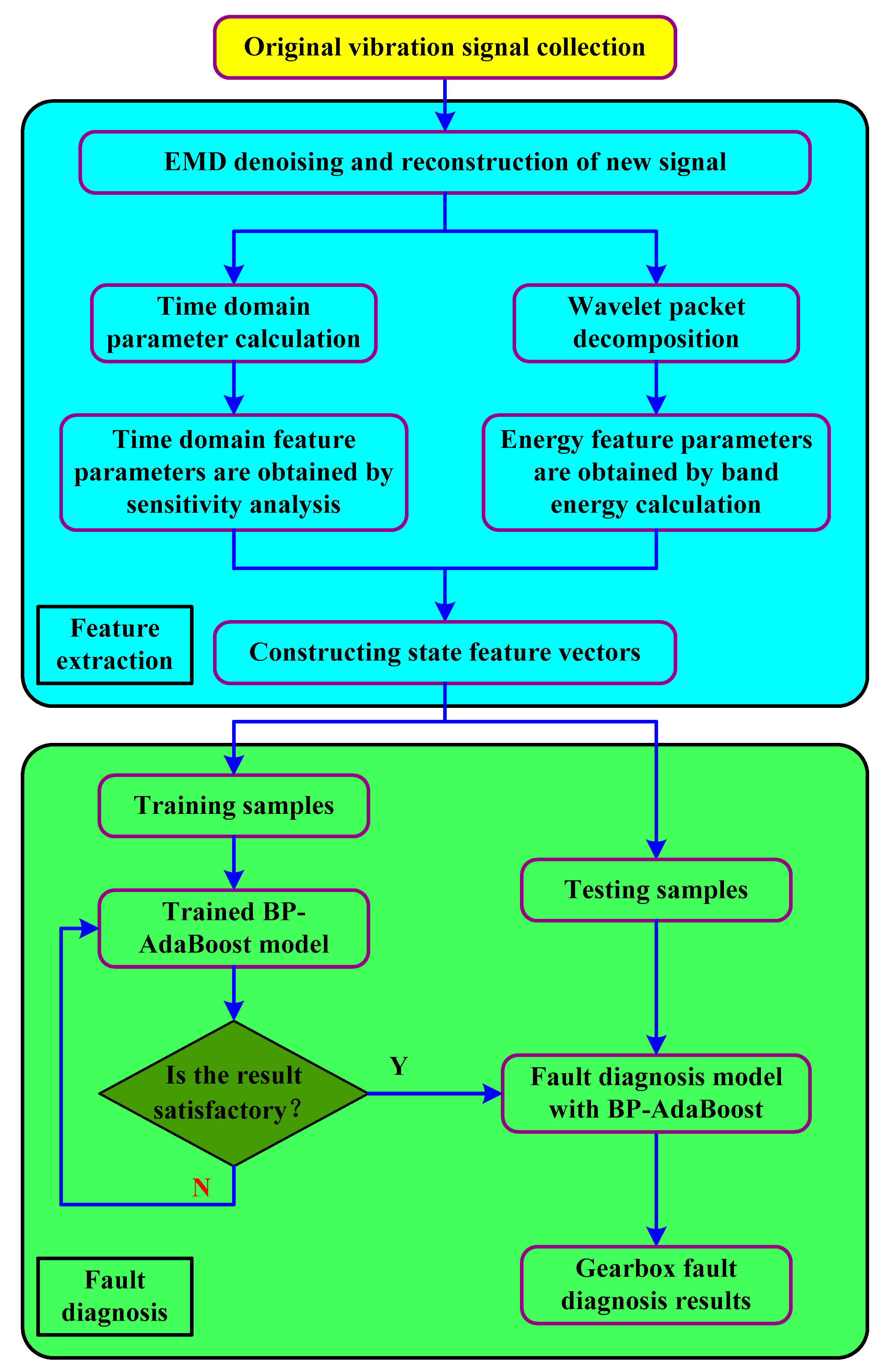
In the context of the above problems and research, in order to use the vibration signal of gearboxes to diagnose the compound fault of gearboxes more effectively, this paper proposes a precise diagnosis method of the compound fault of gearboxes based on multi-feature and BP-AdaBoost. Firstly, empirical mode decomposition (EMD) is introduced to deal with the non-stationary and nonlinear signals in gearbox faults, so as to achieve the purpose of noise reduction; then, time domain analysis and wavelet packet analysis are carried out for the new fault signals after noise reduction processing. In time domain analysis, the sensitivity analysis method can be used to screen out the time domain feature parameters with high sensitivity, and the band energy feature vectors can be obtained through wavelet packet analysis. The two together constitute the state feature vectors that can effectively reflect the running state of the gearbox; finally, AdaBoost algorithm is introduced into the BP neural network model, and the state feature vectors are input into the constructed BP-AdaBoost fault diagnosis model, and finally the precise diagnosis of compound fault of gearbox is realized.
The flow of the proposed method is shown in
Figure 1, which includes the following steps:
Collect vibration signals of the gearbox under different operating conditions, decompose the original vibration signal of gearbox by EMD, and select the appropriate intrinsic mode functions (IMFs) to reconstruct the new signal;
First perform time domain analysis on the reconstructed signal, calculate time domain statistical parameters, and select sensitive time domain feature parameters through sensitivity analysis;
Then, perform wavelet packet analysis on the reconstructed signal, calculate the waveband energy of each frequency band by wavelet packet decomposition, construct band energy feature vectors, and finally form gearbox state feature vectors with the selected time domain feature parameters;
Establish the BP-AdaBoost model, select training samples and test samples, and use the training samples to train the model;
Input the test samples into the trained BP-AdaBoost model to obtain the fault diagnosis results.
The main contributions of the work are summarized as follows:
By combining BP-AdaBoost with sensitivity analysis and wavelet packet analysis, a novel intelligent fault diagnosis method for the compound fault of gearboxes is proposed, which can effectively diagnose the compound fault of gearboxes.
In order to improve the accuracy of fault diagnosis, we improve the traditional fault diagnosis method in three aspects. Firstly, EMD decomposition and reconstruction are used to denoise the signal, then sensitivity analysis is used to select the time domain feature parameters with high sensitivity and combine them with wavelet packet energy feature parameters to form the state feature vector. Finally, BP-AdaBoost is used to build the fault diagnosis model.
The proposed method has certain reference significance and engineering application value for the compound fault of gearboxes as well as other types of faults and machinery.
The rest of this paper is organized as follows.
Section 2 briefly introduces the basic theory of proposed method including EMD, time domain analysis, wavelet packet analysis, and BP-AdaBoost algorithm. In
Section 3, the effectiveness of the proposed method is verified by experiments. Comparative experiments to verify the advantages of the proposed method are presented in
Section 4. Finally, conclusions are drawn in
Section 5.
2. Basic Principle of the Proposed Method
2.1. EMD
The signal of gearbox fault is generally a non-stationary signal, so it is helpful to improve the accuracy of fault diagnosis to adopt the appropriate method to deal with a non-stationary signal. In the process of traditional wavelet analysis, once the wavelet function is selected, it can not be changed according to the actual situation. From this point of view, wavelet transform is not adaptive. Empirical mode decomposition (EMD) is completely adaptive, which does not need to determine the decomposition basis in advance, and is suitable for processing non-stationary and nonlinear signals [
45]. Therefore, the EMD method is used to decompose and reconstruct the original signal to achieve the purpose of denoising.
The EMD method was proposed by Norden E. Huang in 1998. Now, it has been widely used in mechanical fault diagnosis, earthquake research, and medical analysis [
46]. The basic idea of EMD is to decompose the complex signals into many simple ones for the convenience of analysis and research. Its essence is to obtain the intrinsic mode function through the characteristic time scale of data, and then decompose the data. The specific steps of EMD are as follows.
Step 1: determine all local extremum points of the original signal , connect all maximum points and all minimum points with cubic spline curves respectively, and get the upper and lower envelope lines of , so that all data points of the signal are between the two envelope lines.
Step 2: calculate the mean value
of the upper and lower envelope, and subtract
from the original signal
to get
Check whether satisfies the conditions of intrinsic mode function. If not, repeat the above steps with replacement until it is an intrinsic mode function, and record it as the first IMF of the original signal.
Step 3: after decomposing the first intrinsic mode function
from the original signal
, subtract
from
to get the residual value sequence
Step 4: take as the new signal to be processed, repeat the above steps, get IMFs of the original signal in turn, record it as , and then leave the remainder of the original signal.
In this way, the original signal
is decomposed into the sum of several intrinsic mode functions and a remainder:
In order to make the final signal contain the most useful information and the least noise,
IMFs need to be selectively utilized. Add the useful IMFs to get the final reconstruction signal
as the signal to be used, which can be expressed as
2.2. Time Domain Analysis
The time domain diagram of vibration signal records the trend of signal size changing with time in the operation of mechanical system. The time domain signal contains a large amount of information, which is intuitive and easy to understand. It is the original basis of mechanical fault diagnosis. However, the vibration signals collected by the gearbox test-bed are usually non-stationary and non-periodic signals. It is difficult to see the difference between them and normal signals directly from the time domain waveform. Therefore, it is necessary to carry out time domain statistical analysis on the signals, calculate or estimate various time domain parameters and indexes of dynamic signals. By studying and selecting the appropriate time domain feature parameters, we can make accurate judgment for different types of faults.
The feature parameter extraction based on a time domain index refers to the use of the statistical parameters of vibration signals in time domain to characterize the gearbox state information. The advantage of time domain parameters in the field of fault identification is that they can directly describe the gearbox state. Common time domain statistical parameters include: mean (P1), root mean square (P2), square root amplitude (P3), absolute mean amplitude (P4), mean square (P5), maximum (P6), minimum (P7), peak-to-peak (P8), waveform index (P9), peak index (P10), pulse index (P11), margin index (P12), skewness index (P13), and kurtosis index (P14).
In practical application, all kinds of feature indexes have different emphasis on the expression of a fault. Therefore, the above indexes can be used to describe the healthy state of gearbox, which can complement each other and take sensitivity and stability into account.
In the process of time domain analysis, multiple time domain feature parameters will be extracted. The sensitivity of the selected feature parameters to the fault determines the difficulty and accuracy of fault diagnosis. Therefore, it is very important to select the appropriate feature parameters to form the fault feature vector [
47]. Therefore, it is necessary to analyze the sensitivity of these parameters after extracting the time domain feature parameters, and screen out the feature parameters which can effectively represent the state of gearbox. The calculation formula of sensitivity analysis is
where
is the sensitivity,
is the parameter to be analyzed, and
is the reference parameter. Usually, the time domain feature parameters of normal state are taken as reference parameters, and the time domain feature parameters of fault state are taken as parameters to be analyzed. Note that sensitivity analysis is a normalization process although it is used as a means for parameter selection.
2.3. Wavelet Packet Analysis
Wavelet transform is one of the most popular time-frequency transform methods that has the ability to characterize signal characteristics in both time and frequency domain. At present, wavelet transform is widely used in the field of rotating machinery fault diagnosis [
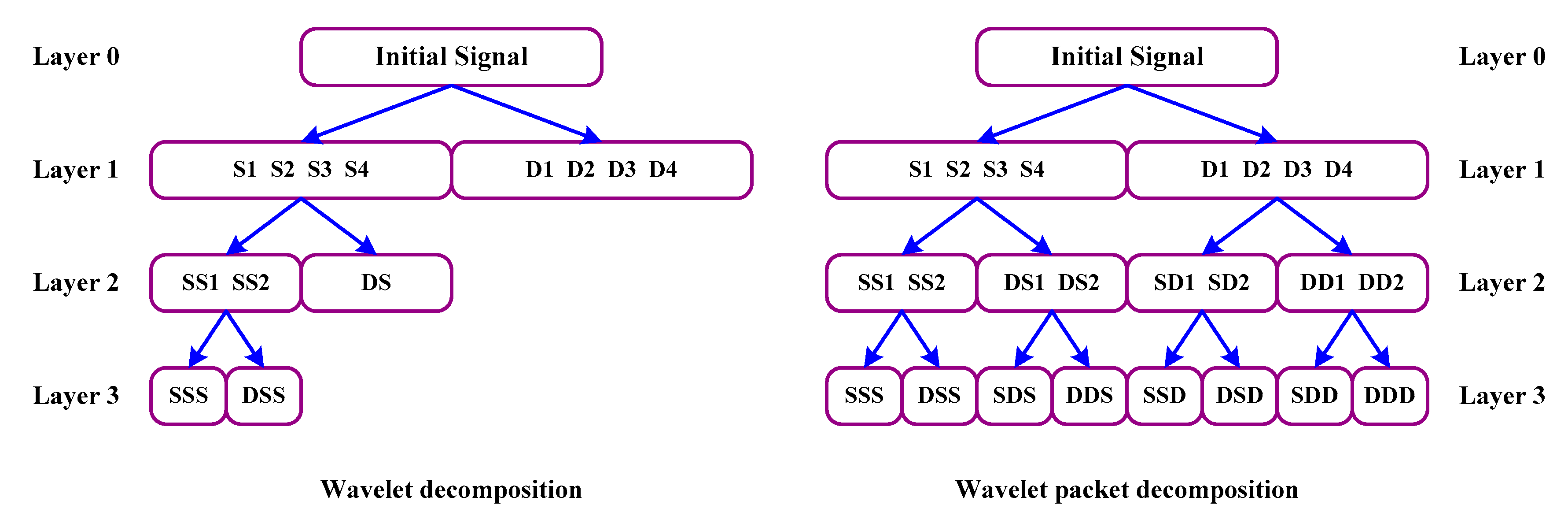
48]. However, the decomposition method adopted by wavelet decomposition has poor time resolution in the low frequency band and poor frequency resolution in the high frequency band. In order to solve this problem, wavelet packet analysis provides the way to solve the problem; it is the extension of wavelet analysis and is a more precise method of signal analysis. It not only inherits the advantages of time-frequency localization of wavelet transform, but also further decomposes the high frequency band that are not re-decomposed by the wavelet transform, so as to improve the frequency resolution. The comparison figure of frequency band division between wavelet decomposition and wavelet packet decomposition is shown in
Figure 2. Obviously, wavelet packet decomposition has symmetrical characteristics. S represents the low frequency part of a vibration signal and D represents the high frequency part of a signal.
For the key components such as gearbox, wavelet packet analysis can fully capture the useful information in the vibration signal, which is conducive to accurate diagnosis, so wavelet packet decomposition is more reliable and feasible. The principle of wavelet packet decomposition is as follows.
If the original signal collected is
(subspace formed by orthogonal sum of wavelet subspace and scale subspace), then
can be represented by wavelet packet decomposition:
where
is scale,
is translation factor,
is basis function in subspace
,
is coefficient of wavelet packet decomposition, and
can be decomposed into
and
by a formula, that is,
where
is the scale in the decomposition process and
is the wavelet coefficient.
After the vibration signal of gearbox is decomposed by a frequency band in the above way, each node will arrange the final result according to the frequency band, but it is difficult to judge the operation state of gearbox intuitively through the sub-band information of wavelet packet decomposition, and the energy value of the vibration signal in different frequency bands is different, which can effectively extract the information contained in each frequency band of the signal. Therefore, the failure mode of the gearbox can be identified by calculating the energy of each frequency band of the signal.
Suppose that the highest frequency of the vibration signal is . By performing wavelet packet decomposition of -layer on , we can get groups of wavelet packet coefficients, which are , respectively. The corresponding frequency band of groups of coefficients is .
According to Parseval’s theorem, the energy calculated in a time domain is consistent with that calculated in a frequency domain, so the energy calculation formula of each frequency band is
Taking
as the element can form an energy feature vector such as
. In practical applications, the energy of each node is usually normalized, that is, the proportion of the energy of each node to the total energy is taken. Let
, and the energy feature vector can be normalized as:
2.4. BP-AdaBoost Algorithm
A back propagation neural network (BP neural network, BPNN) has excellent nonlinear approximation characteristics, and has been widely used in many fields, but there are also some defects, such as being easy to fall into local minima and not being able to get the global optimal solution, resulting in a low recognition rate of mechanical equipment failure mode. The AdaBoost algorithm is introduced into a BP neural network model to build a BP-AdaBoost fault diagnosis model, which can effectively improve the diagnosis accuracy of the original single BP neural network.
The AdaBoost (Adaptive Boosting) lifting method is one of the most classical methods in the boosting algorithm family. It reduces the error rate through the adaptive learning method [
49]. The main idea of the algorithm is: first, each sample is initialized to equal weight, and then iterates
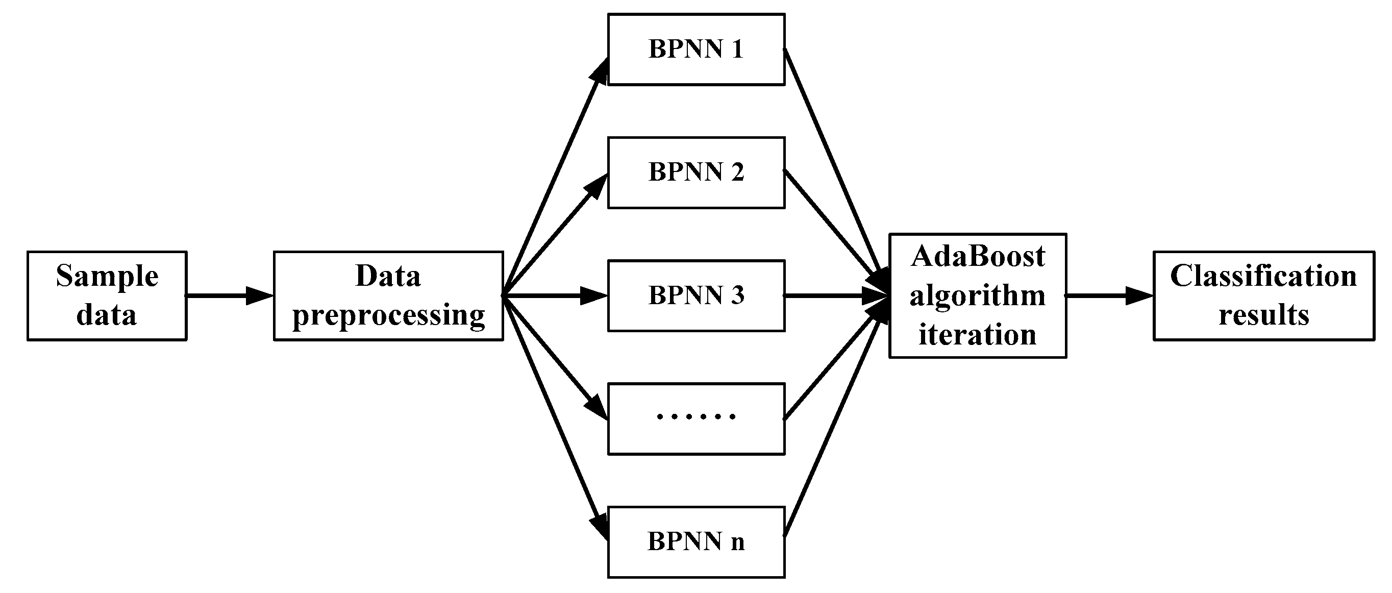
n times with a weak classifier. After each iteration, the weight is updated according to the classification results. For the failed samples, a larger weight is given, and more attention is paid to the next iteration. Weak classifiers get a sequence of classification functions through multiple iterations. Each classification function will give a certain weight according to the classification error, and finally combine multiple weak classifiers to form a strong and stable classifier with small classification errors. The algorithm flow of BP-AdaBoost is shown in
Figure 3, and its main steps are as follows.
Step 1: data selection and network initialization. Select group training samples from the sample space and initialize the sample weight . According to the dimensions of sample input and output, the structure of neural network is determined, and the weight and threshold of BP neural network are initialized.
Step 2: weak classifier prediction. When training the
weak classifier, the BP neural network is trained with the training data, and the output of the training result is predicted. The prediction sequence
and the prediction error sum
are obtained:
where
and
are predicted classification results and expected classification results, respectively.
Step 3: calculate the weight
of the prediction sequence according to the prediction error
. The formula is
Step 4: update the training sample weight. Adjust the weight of training samples in the next round of training according to the prediction sequence weight
, and the adjustment formula is
where
is the normalization factor, the purpose is to keep the weight proportion unchanged and the sum of the weights equal to 1.
Step 5: synthesize a strong classifier. After training
rounds, we get
groups weak classification function
, and combine them to get a strong classification function:
3. Experimental Verification and Analysis
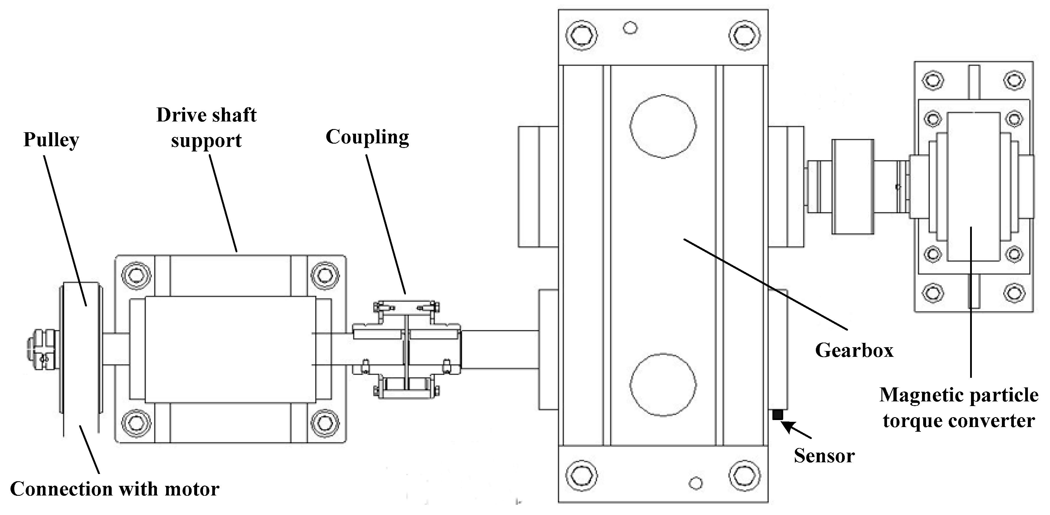
In order to verify the effectiveness of the proposed method, the gearbox preset fault experiment is specially set for data verification. A QPZZ-II rotating machinery vibration analysis and fault diagnosis experimental platform system is adopted in the experiment, and the structural diagram of the experimental platform is shown in
Figure 4. The gearbox used in the experiment is mainly composed of a pair of meshing gears. The big gear is the driving wheel, the number of teeth is 75, the small gear is the driven wheel, the number of teeth is 55, and the module is 2. The speed range of the motor is 75–1450 rpm, and the maximum workload is 5 N·m. The acquisition software of the system can realize the signal acquisition and storage.
According to the analysis of common failure modes of gearbox, this experiment simulates six operation states of gearbox, and the specific experimental settings are shown in
Table 1.
During the experiment, the acceleration monitoring data in the y-direction on the load side of a gearbox input shaft is collected by an acceleration sensor, and the sampling frequency is 5120 Hz. The signal with a length of 5120 points each time is taken as a sample, so the time length of this signal is 1 s, and the sample contains the state information of the gearbox within 1 s, and the rotational speed of the gearbox is 880 rpm, so this signal can effectively contain all the information of the gearbox within one operation cycle.
3.1. Denoising with EMD
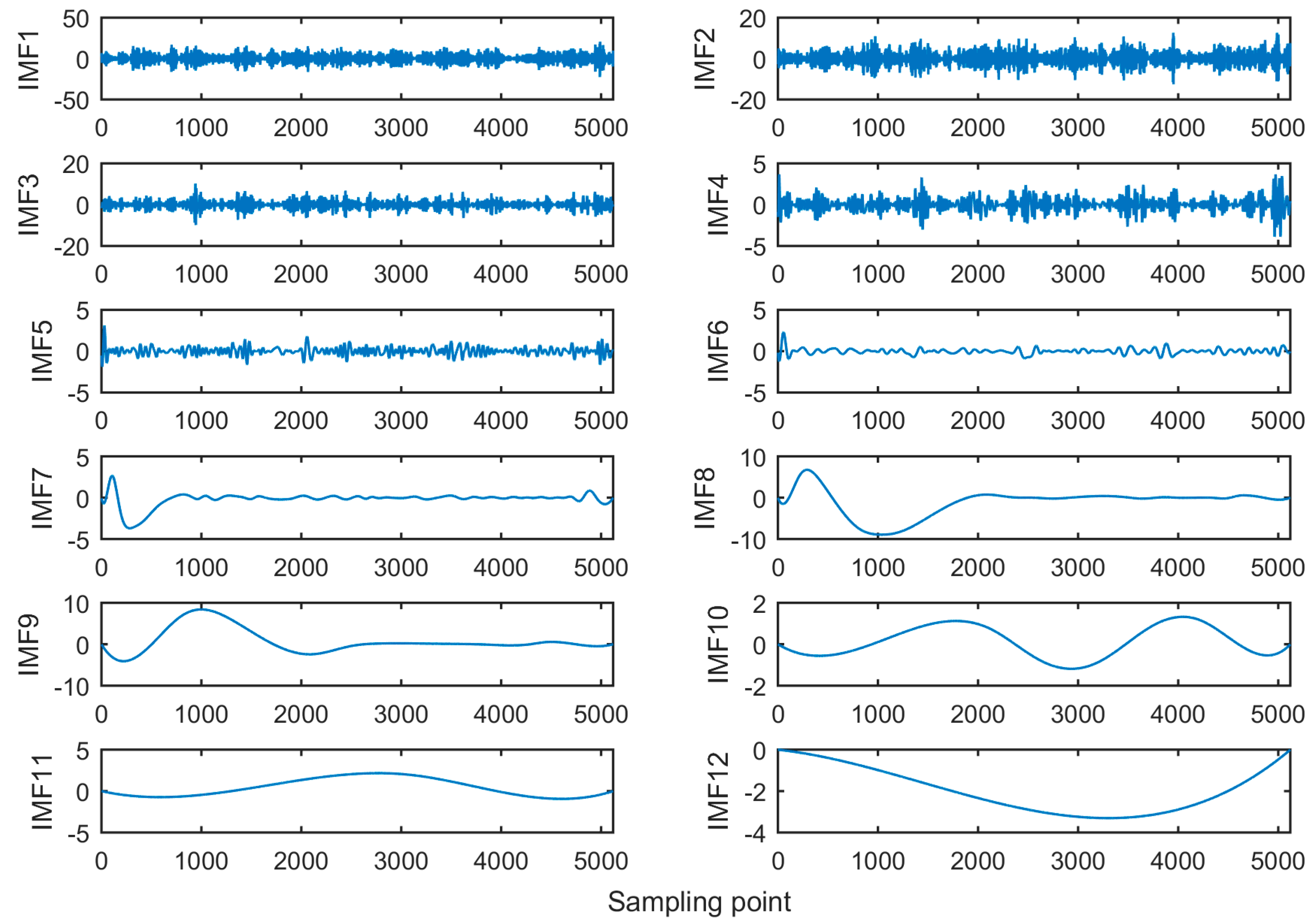
The original signal collected is decomposed by the EMD method, and the decomposition result is shown in
Figure 5. In the figure, 12 IMFs of the signal are successively from top to bottom.
From Ref. [
45], if the higher the ratio of energy of IMF obtained by EMD to that of an original signal, the higher the similarity between IMF and original signal, the more useful information it contains.
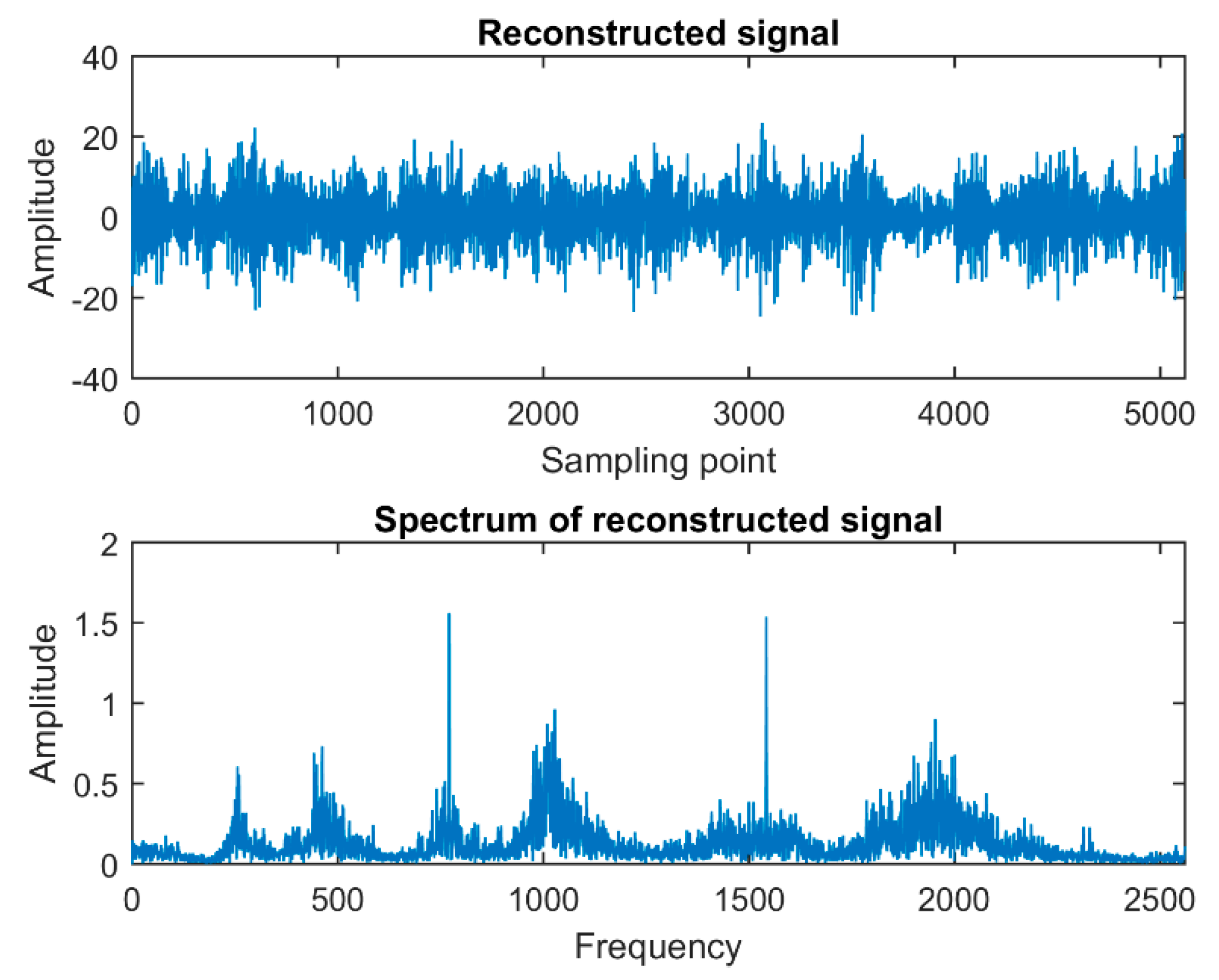
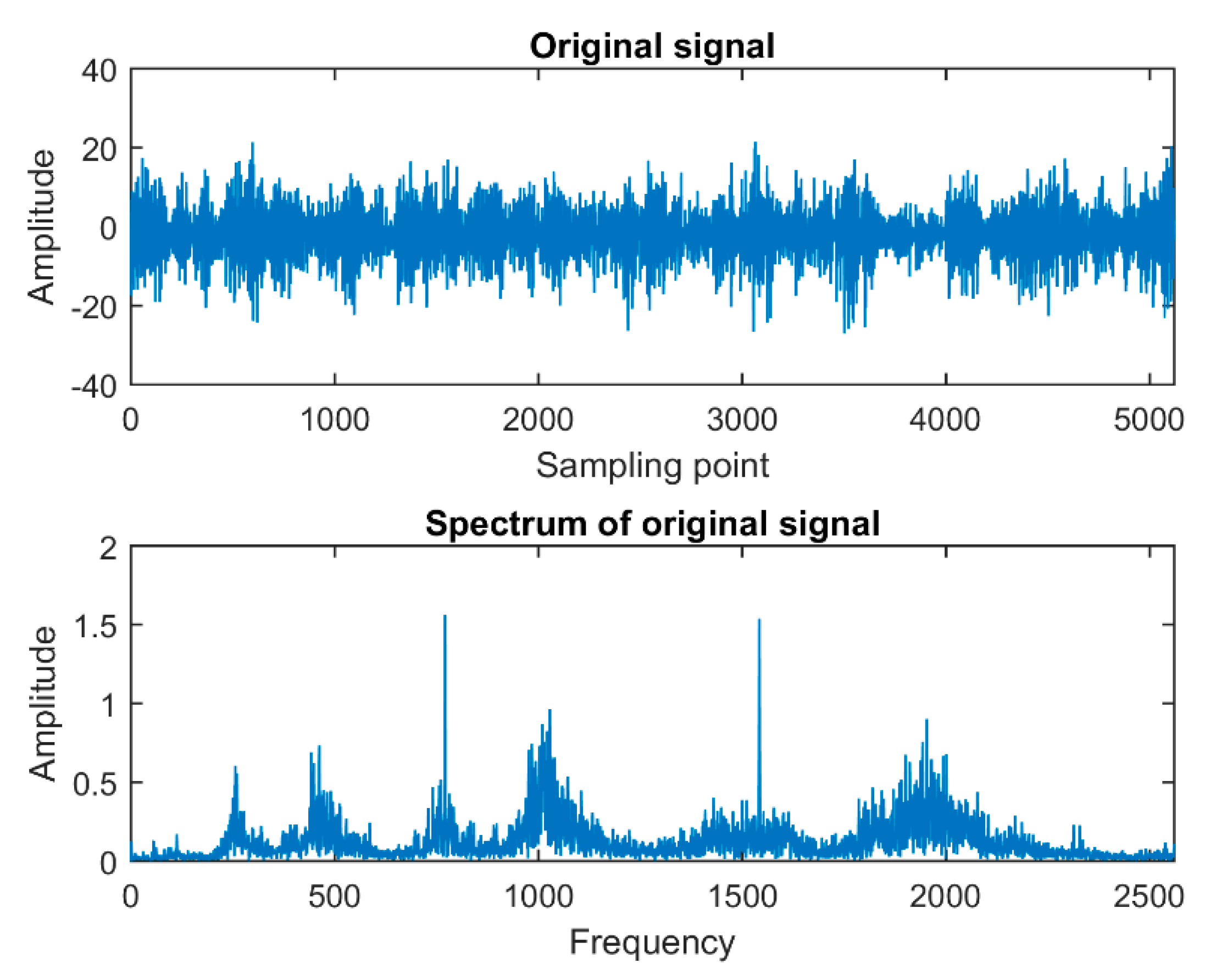
After analysis and calculation, it can be known that, among the 12 IMFs obtained by the above decomposition, the first four IMFs occupy a relatively high energy of the original signal, so these four IMFs are selected as the IMFs of the reconstructed signals. The first four IMFs are added and reconstructed to obtain a new fault signal. The time domain diagram and spectrum diagram of the reconstructed signal are shown in
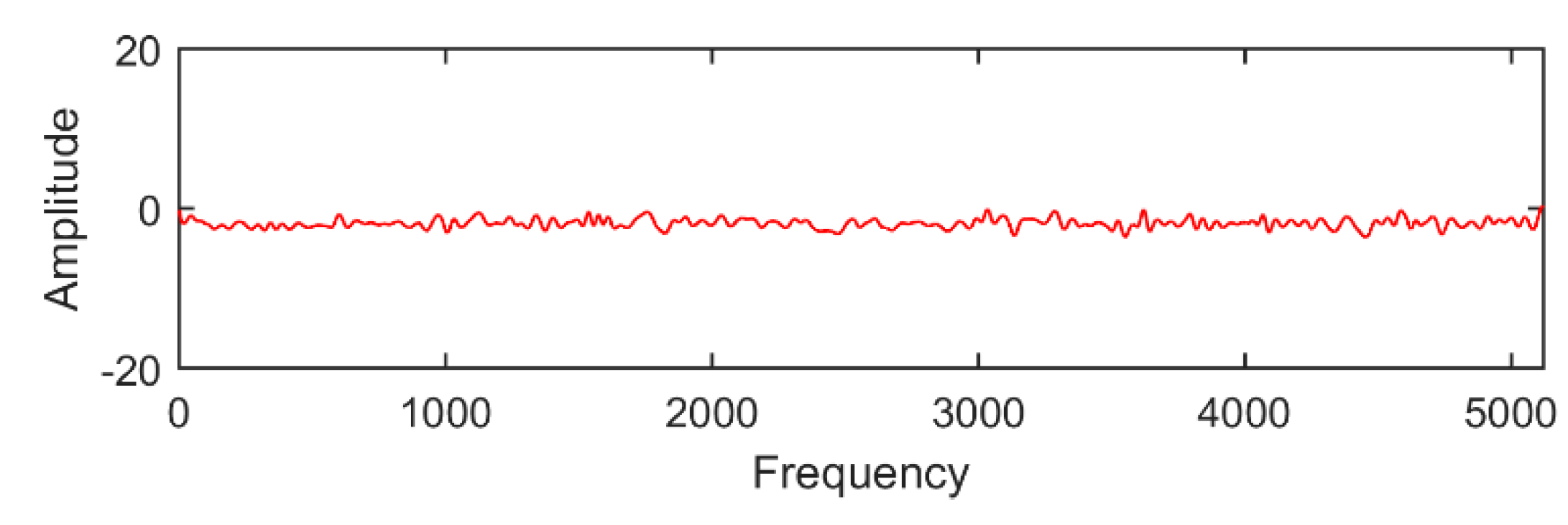
Figure 6. At the same time, the time domain diagram and spectrum diagram of the original signal and the error diagram of the reconstructed signal and the original signal are made, as shown in
Figure 7 and
Figure 8, respectively.
Through comparison, it can be found that the similarity between the new signal reconstructed by the first four IMFs and the original signal is very high, which can hardly be seen by human eyes. This is also verified in the reconstruction error diagram, which shows that the reconstructed signals retain most of the useful fault information of the original signals, and achieve the purpose of removing noise. Therefore, the reconstructed signal can be used as a new fault signal to extract fault feature parameters.
3.2. Time Domain Analysis of a Gearbox Vibration Signal
In order to extract fault information more comprehensively and effectively, 14 common time domain statistical parameters are selected as the candidate parameters. Extract the time domain feature parameters of the above new fault signals processed by the EMD method, and get the feature parameters of normal state and five fault states, respectively, as shown in
Table 2.
Each feature parameter can reflect certain fault information. The above 14 candidate feature parameters reflect different fault information from different aspects, but their sensitivity to different operating states is different. Because there is a certain correlation between the parameters, and too many parameters will inevitably lead to a large increase in the amount of calculation due to the “dimension effect”, it is necessary to carry out sensitivity analysis on 14 candidate feature parameters to screen out the feature parameters with better sensitivity, which is more conducive to the recognition of the working state of the gearbox.
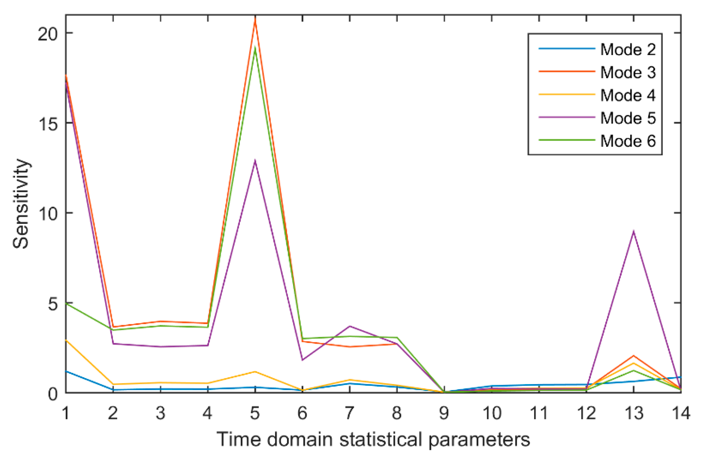
Sensitivity analysis is carried out for 14 candidate feature parameters, and the analysis results are shown in
Figure 9.
In
Figure 9, each polyline represents the average sensitivity of each feature parameter in a fault state. For the sensitivity of a feature parameter, the larger the value in a certain failure mode, the more the feature parameter is conducive to distinguishing between normal status and failure mode. When selecting the appropriate feature parameters, not only the ability of the feature parameters to distinguish between normal and fault states, but also the ability of the feature parameters to identify different fault modes.
It can be seen from
Figure 9 that the first feature parameter (P1), the fifth feature parameter (P5), and the 13th feature parameter (P13) are highly sensitive, and the differences between different fault modes are relatively large. The ability to recognize different states of the gearbox is better. Therefore, the three feature parameters of mean (P1), mean square (P5), and the skewness index (P13) are selected as the time domain feature parameters of gearbox fault.
3.3. Wavelet Packet Analysis of a Gearbox Vibration Signal
Time domain indicators can characterize part of the gearbox fault information. However, using only time domain feature parameters as feature vectors, errors in gearbox fault diagnosis results are usually very large. Therefore, it is necessary to use the signal processing technology to analyze the fault signal to obtain new fault feature parameters, and together with the fault feature parameters in the time domain to form the gear box fault feature vector.
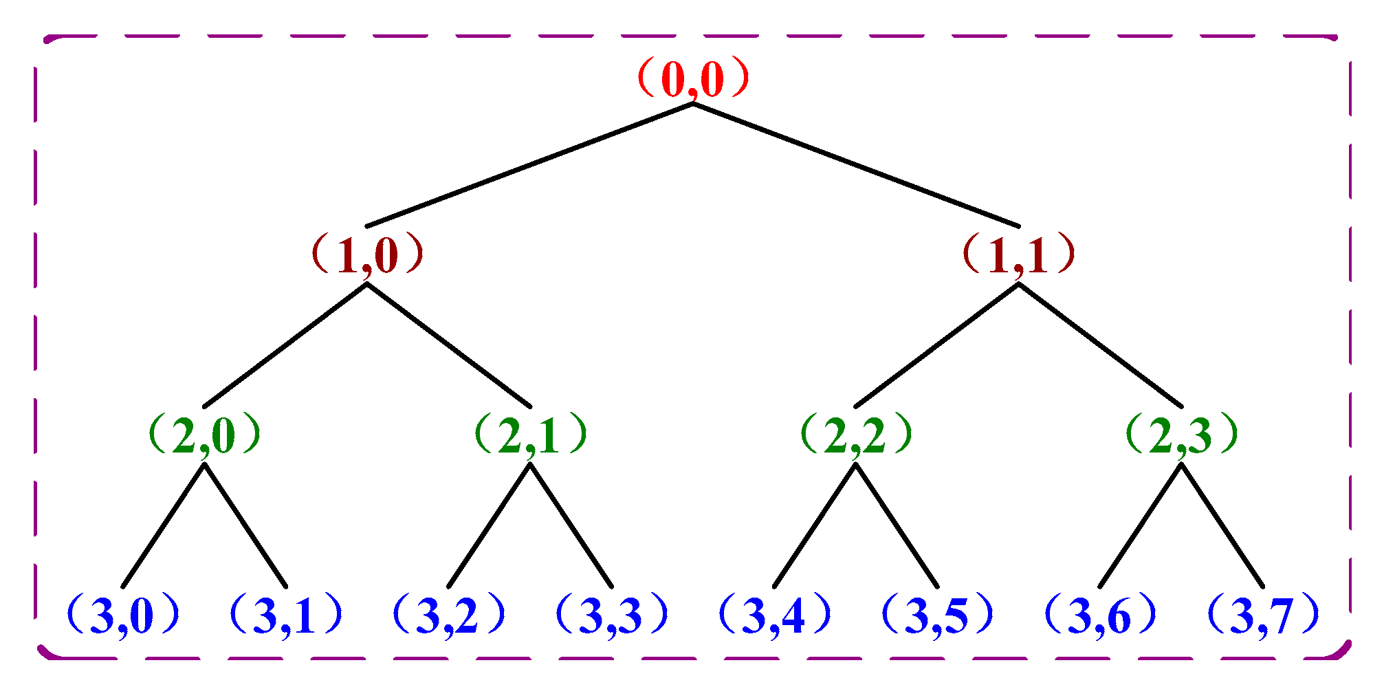
According to relevant theories and many times of practice, compared with other wavelet functions, the wavelet basis functions based on Daubechies (db wavelet) are more suitable for analyzing the vibration signals of gearboxes, and their performance is best when the number of wavelet
n = 5. Therefore, this paper selects Daubechies5 (called db5 wavelet) as the wavelet basis function for gearbox signal analysis, and then uses the db5 wavelet basis to perform three-layer wavelet packet decomposition on the data, and decomposes to obtain eight subbands. The wavelet packet decomposition tree structure and decomposition results are shown in
Figure 10 and
Figure 11, respectively.
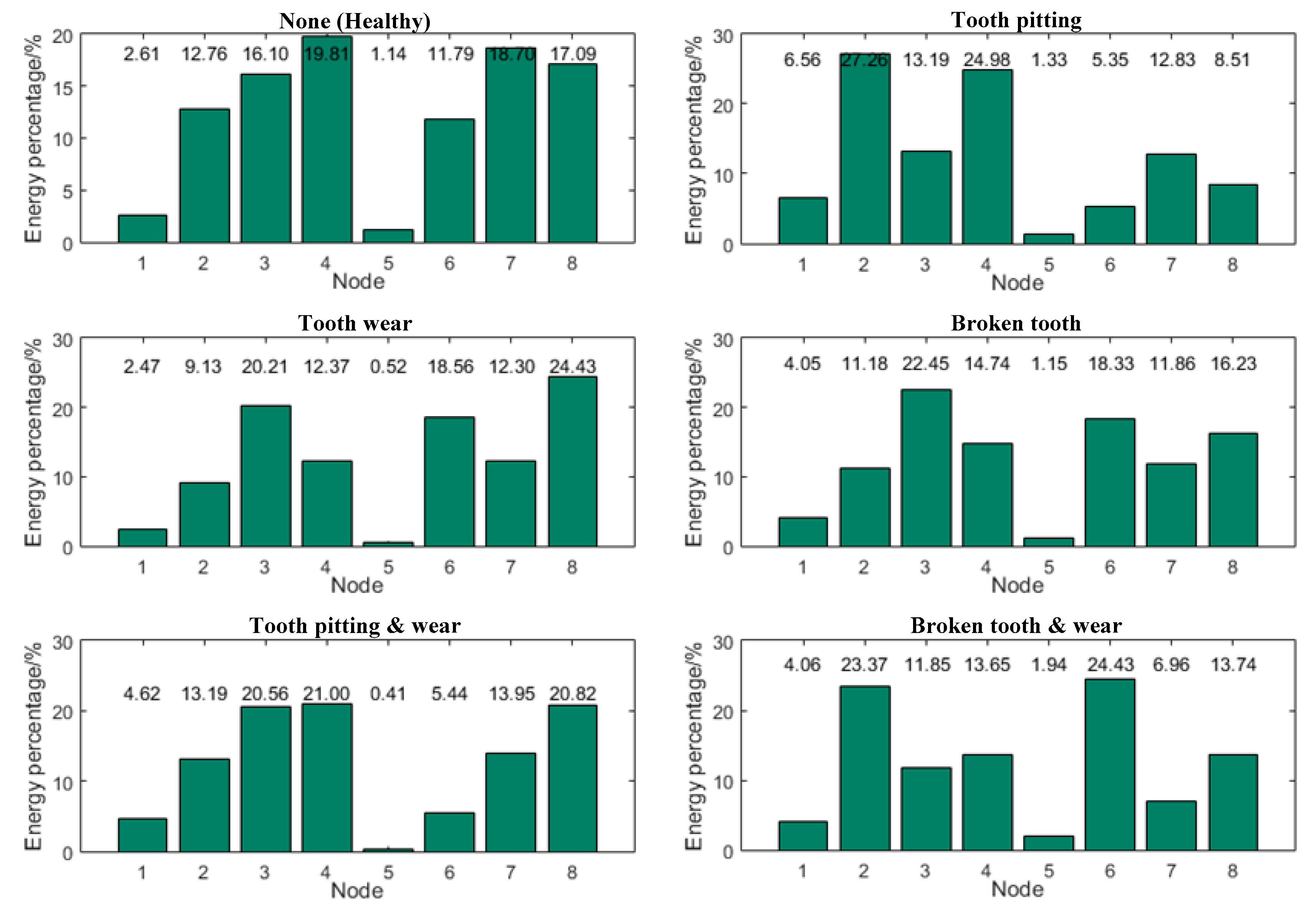
After the wavelet packet decomposition results are obtained, the energy of each frequency band in six states of gearbox is calculated, and the normalized energy values of each frequency band are used to form the energy characteristics. The frequency band energy distribution in each state is shown in
Figure 12.
As can be seen from
Figure 12, under different operating conditions of the gearbox, the energy characteristics of each frequency band of the vibration signal have significant differences, so it can provide an effective basis for identifying the operating state of the gearbox.
Combining the eight wavelet packet energy features with the three-time domain feature parameters obtained in the time domain analysis, the 11-dimensional gearbox state feature vector is constructed. In this experiment, 160 sets of data are collected for each state of gearbox. Therefore, after the above feature extraction, 160 sets of 11-dimensional gearbox state eigenvectors are obtained for each state. Some of the state feature vector parameter values are shown in
Table 3.
3.4. Gearbox Fault Diagnosis Based on BP-AdaBoost
Firstly, the BP-AdaBoost fault diagnosis model is established. According to the dimension of data and the general rule of determining the number of neurons in the hidden layer, the structure of BP neural network is 11-6-1. At the same time, considering the requirements of calculation time and diagnosis accuracy, the number of weak classifiers is 10, and then 10 weak classifiers are used to form a strong classifier to classify the operation state of the gearbox.
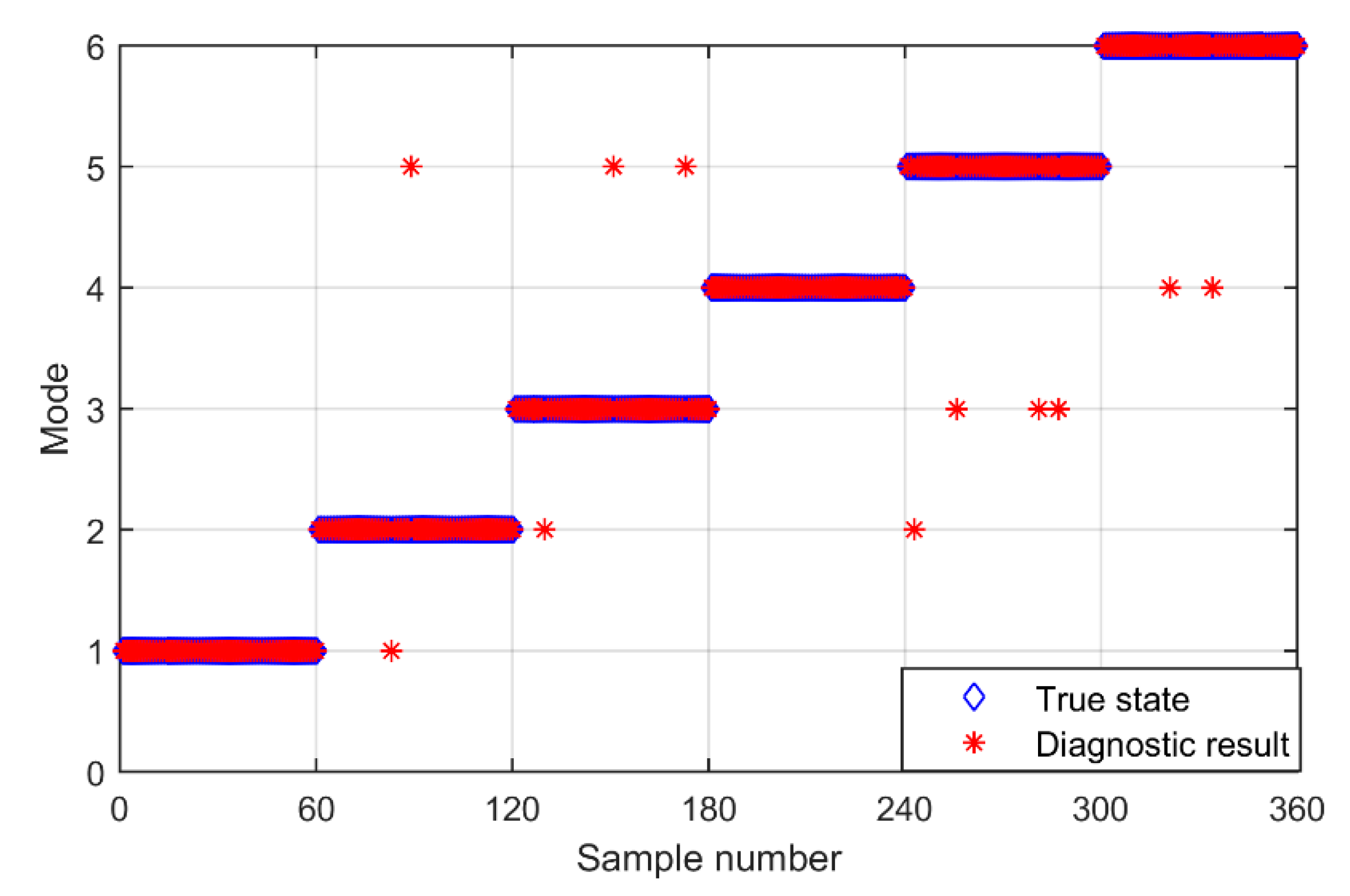
Among the 160 sets of state feature vectors of each of the above states, 100 groups are randomly selected as training samples, and the remaining 60 groups are used as test samples. The training samples of each mode are input into the established BP-AdaBoost fault diagnosis model in turn, and the BP-AdaBoost model is trained. After training is completed, input the test samples and then get the test results as shown in
Figure 13. The test results are statistically calculated, and the diagnostic accuracy of the BP-AdaBoost fault diagnosis model is calculated as shown in
Table 4.
From the above diagnosis results, it can be seen that, on the basis of extracting the multiple features of the compound fault of gearboxes, the recognition accuracy of the gearbox fault mode using BP AdaBoost fault diagnosis model is relatively high, and two groups have achieved all the correctness, and the overall accuracy is close to 97%, which verifies the feasibility and effectiveness of the method proposed in this paper.
4. Comparison Experiment and Discussion
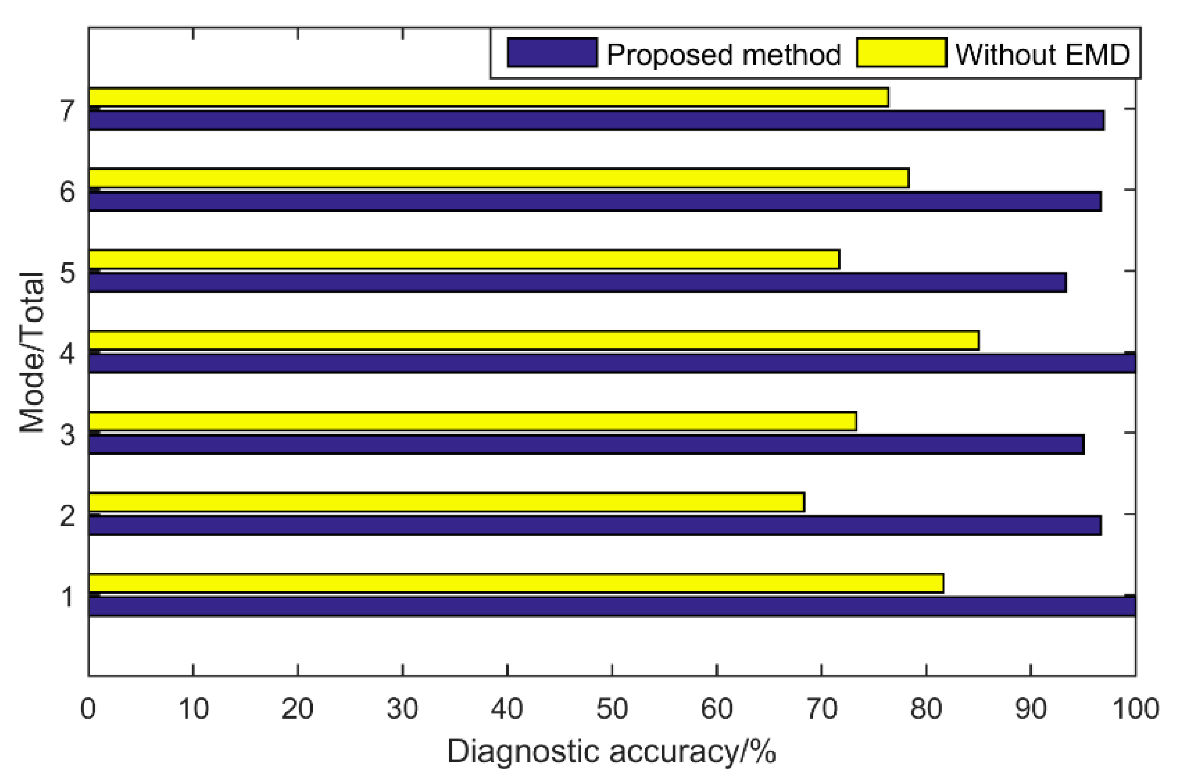
In order to further verify the superiority of the proposed method in gearbox compound fault diagnosis, comparative experiments are needed. In the first round of comparative experiments, the original signal is not processed by the EMD method, and the time domain analysis and wavelet packet analysis are directly performed to obtain the gearbox state feature vectors. Then, the same fault diagnosis model is used. The comparison chart is shown in
Figure 14.
Through comparative analysis, it can be clearly found that the accuracy rate of the feature parameters extracted from the reconstructed vibration signal after the original vibration signal is decomposed and reconstructed by EMD is significantly higher than the accuracy rate of feature parameters extracted for fault diagnosis without EMD processing, which shows that, in the process of processing the vibration signal of the gearbox, EMD achieves the purpose of denoising, and, at the same time, the reconstructed signal contains as much useful information as possible, which can improve the signal-to-noise ratio and thereby facilitate fault diagnosis.
In the second round of comparative experiments, based on the EMD decomposition of the original vibration signal and the reconstruction signal, different feature parameters are extracted, including the time domain feature parameters, the frequency domain feature parameters, and the frequency band energy feature parameters of wavelet packet decomposition. These parameters are composed of 3D time domain feature vectors, 3D frequency domain feature vectors, and 8-dimensional energy feature vectors, respectively. Then, they are respectively input in some traditional fault diagnosis models, such as BP neural network (BPNN) and support vector machine (SVM), the final fault diagnosis results are summarized as shown in
Table 5.
A number of meaningful conclusions can be clearly drawn from
Table 5. First of all, for the same fault diagnosis method, the diagnosis accuracy rate is the highest when multi-feature vectors are used. When only frequency domain feature vectors are used, the accuracy is only about 50%. This is because the characteristic frequencies between compound faults of the gearbox are relatively close. It is difficult to identify the compound fault mode of the gearbox based on the frequency domain characteristics. Therefore, this paper uses a combination of sensitive time domain feature parameters and energy feature parameters. In addition, when multi-feature vectors are used at the same time, the diagnostic accuracy of the proposed method is higher than that of traditional fault diagnosis methods. Taking BPNN as an example, due to the existence of local minimum points, it can not guarantee that the network will eventually converge to the global minimum point. Therefore, the overall classification recognition effect is relatively low, and the diagnostic accuracy of the similar compound fault mode is the lowest. It should also be noted that the initialization of weights may affect the final convergence of the network, resulting in some results with strong randomness, and the diagnostic results differ greatly each time. However, BP-AdaBoost can fully take advantage of the adaptive learning method in the AdaBoost lifting method to reduce the error rate. The strong classifier formed by integrating multiple weak classifiers has small and stable classification errors.
5. Conclusions
In this paper, a diagnosis method for the compound fault of gearboxes based on the combination of multi-feature vectors composed of sensitive time domain characteristic parameters and band energy characteristics by wavelet packet decomposition and BP AdaBoost algorithm is proposed. The following conclusions can be obtained through the experiments and simulation results. By collecting and analyzing the vibration signal of the gearbox, the running state of the gearbox can be effectively monitored. Decomposing the original vibration signal of gearbox by EMD and selecting the appropriate IMFs to reconstruct the new signal can achieve the purpose of denoising the original signal. Multiple time domain statistical parameters are calculated from the time domain analysis. Through the sensitivity analysis, the time-domain characteristic parameters that can effectively reflect the fault state can be selected, so as to avoid the overlapping or interference of multiple parameters and reduce the calculation amount. Among them, the sensitivity of mean, mean square value, and the skewness index is higher, and the ability to identify different operation states of gearbox is better. Wavelet packet decomposition is an effective feature extraction method of a gearbox vibration signal, which can extract the feature information of a vibration signal in each frequency band, and the feature vector composed of energy in each frequency band can well characterize the operation state of gearbox. The combination of the time domain feature parameters and the frequency band energy feature is used as the state feature vector of the gearbox, and the accuracy of diagnosis is close to 97% when it is input into the BP-AdaBoost fault diagnosis model, which proves the effectiveness of the method proposed in this paper. Compared with the traditional fault diagnosis methods, the advantages of the proposed method can be found. Therefore, the proposed method has great potential for online or offline fault diagnosis of a gearbox compound fault, which can effectively avoid serious accidents, ensure the safe operation of equipment, and improve economic benefits. However, it should be noted that the method proposed at present is only for the typical fault of the gear in the gearbox, but the gearbox also contains the bearing and shaft and other components, which are likely to fail, so future work will focus on solving the problem of compound fault diagnosis of multiple components in the gearbox.


