Multibody System with Elastic Connections for Dynamic Modeling of Compactor Vibratory Rollers


1
Research Institute for Construction Equipment and Technology—ICECON SA, 021652 Bucharest, Romania
2
Faculty of Engineering and Agronomy, “Dunărea de Jos” University of Galaţi, 810017 Brăila, Romania
Symmetry 2020, 12(10), 1617; https://doi.org/10.3390/sym12101617
Submission received: 21 August 2020
/
Revised: 14 September 2020
/
Accepted: 25 September 2020
/
Published: 29 September 2020
(This article belongs to the Special Issue Multibody Systems with Flexible Elements)
Abstract
:The dynamic model of the system of bodies with elastic connections substantiates the conceptual basis for evaluating the technological vibrations of the compactor roller as well as of the parameters of the vibrations transmitted from the vibration source to the remainder of the equipment components. In essence, the multi-body model with linear elastic connections consists of a body in vertical translational motion for vibrating roller with mass m1, a body with composed motion of vertical translation and rotation around the transverse axis passing through its weight center for the chassis of the car with mass m and the moment of mass inertia J and a body of mass m’ representing the traction tire-wheel system located on the opposite side of the vibrating roller. The study analyzes the stationary motion of the system of bodies that are in vibrational regime as a result of the harmonic excitation of the m mass body, with the force , generated by the inertial vibrator located inside the vibrating roller. The vibrator is characterized by the total unbalanced m0 mass in rotational motion at distance r from the axis of rotation and the angular velocity or circular frequency ω.
1. Introduction
The real-time assessment of the degree of compaction of the foundation soil both with stabilized natural soil as well as mixed with stone mineral aggregates or in the case of compaction of asphalt concrete layers, requires precision and high sensitivity of the dynamic response in amplitude of the compactor roller to the changes of soil rigidity as a result of the compaction process.
After each passage on the same compacted layer, the final rigidity of the soil has a new value, higher than the initial rigidity. In this case, after each passage, there can be estimated, through an appropriate instrumental system, the modified amplitude of vibration in correlation with the new state of compaction of the soil corresponding to modified rigidity.
Currently, there are several companies manufacturing vibration compactor machines that use instrumental and computer systems for capturing, treating, and processing the specific signal to the vibration of the vibrating roller. Usually, the dynamic calculation model used is reduced to that of the vibrating roller system with a single degree of freedom, without taking into account the effect of the other vibrating moving masses of the machine.
Frequently, for vibration regime at frequencies in the range of 40–50 Hz, the system ensures the degree of compaction in real time based on the change in rigidity with each passing on the same layer of land. In this case, the first two resonant frequencies are neglected, although they may be important in the work process.
At frequencies between 15 and 30 Hz, the automatic analysis of technological vibration systems produce errors 30% larger, which leads to major inconveniences. For these reasons, the current dynamic study highlights the influence of the masses of the body assembly at various dynamic regimes for functional frequencies from 15 Hz to 80 Hz. According to the category of the compaction technology, that is, the change in final rigidity after each passage of the compacted layer, there are many scientific and technical approaches with case studies on technologically defined sites that require a more complete dynamic approach, highlighting the influences of the body system on the dynamic response and of the degree of compaction [1,2].
2. Multibody System Model
The dynamic multibody model of the vibrating roller is presented in Figure 1 [4,5,6], where the following notations are used:
I1—elastic connection point of the vibrating roller with vertical translational movement;
I2—connection point of the elastic system to the front side of the car chassis;
I3—connection point between the rear of the car chassis to the traction unit consisting of tire-wheels;
m’—mass of the vibrating roller;
m—mass of the car chassis;
J = Jz—moment of mass inertia in relation to the transverse axis z passing through the center of mass C of the car chassis;
m1—mass of the traction group;
k1—rigidity of the compacted material;
k2—rigidity of the elastic connection system and dynamic insulation between the vibrating roller and the front chassis;
k3—combined rigidity of the traction wheel tires in contact with the compacted material;
a, b—distances of the C mass center in relation to the I2 and I3 ends of a chassis, so that a + b = l, where l = I2I3 is the equivalent length of the chassis;
x, φ = φz—instantaneous displacements of the chassis; and
x1, x2, x3—absolute instantaneous displacements relative to a fixed reference system.
Instantaneous displacements of points i = 1, 2, 3, can be determined with the following matrix relation [7,8]:
where x, y, z are the tri-orthogonal instantaneous linear coordinates of the mass center belonging to each rigid body I1 and C, respectively.
—the tri-orthogonal instantaneous angular coordinates relative to the competing x,y,z axes in the center of mass of each rigid body C1 and C2, respectively.
For the m1 mass body with vertical translational motion and the null instantaneous angular coordinates, that is , the displacement of the I1 ≡ C1 point is
For the mass body m and moment of inertia Jz = J, with the instantaneous angular coordinates and , it has a plane motion (x, ), so that the displacements of points I2 and I3 can be determined as follows:
2.1. Kinetic Energy of the Multibody System
Taking into account the motion of body C1 of mass m1 with translation coordinate x1 and of the assembled body C2C3 with mass m + m’, moment of mass inertia , with coordinates x, φ (vertical translation and rotation), the kinetic energy of the assembly of bodies is [9,10]
where is the column vector of the generalized velocity with ;
M—symmetric and positively defined inertia matrix; and
—scalar product between vectors and .
Matrix M of the entire system of instantaneous moving bodies with generalized coordinates x1, x, and φ, consists of inertial elements of zero order m1, m + m’, one order m’b and two order , placed on the main diagonal and symmetrically in relation to it, highlighting an inertial coupling due to a C3 body eccentrically assembled on body C2. In this case, matrix M can be written as follows:
The analytical expression of the kinetic energy, based on relations (5) and (6), can be developed in the form of
where the following notations were used for the inertia coefficients m2, m3, and m23, so ; ; .
2.2. Elastic Potential Energy
For the elastic elements, modeled as linear springs with rigidities k1, k2, k3, the vector of the elastic deformations v, with has the following components [7,11]:
Thus, vector v can be written as
The transition from the elastic deformations vector to the vector of instantaneous displacements with can be done by the linear transformation of
where A is the matrix of the linear transformation as an operator of influence of the displacements on deformations.
Taking into account relations (9) and (10), matrix A can be formulated as follows:
The potential elastic energy can be formulated based on the use of the scalar product between vectors v and K0v, where , as follows:
Using the linear transformation (10) where A has the property of a self-adjoint operator inside the scalar product, relation (12) becomes
or
where K is the rigidity matrix of the multibody elastic system.
In this case, matrix can be written as
It is found that matrix K is symmetrical and positively defined with elastic coupling elements symmetrically placed in relation to the main diagonal. In general form, matrix K can be written as follows:
where elements kij are those in formulation (15), that is:
The potential elastic energy in analytical form, in this case, can be formulated in the form of , as follows
Elastic force Qj, which corresponds to the generalized coordinate qj can be written as follows:
In this case, deriving the relation (16) in the form of in relation to coordinate , that is leads to , and thus we obtain
Taking into account function in relation (16) and the fact that and , applying relations (18), we obtain
2.3. Disruptive Force
The harmonic excitation is given by the disruptive force , where the amplitude of the force is . This is applied on body C1 in order to generate forced vibrations in the vertical direction so that the mass body m1 and coordinate x1 only have vertical translational movement.
In this case, the vector of disruptive forces is
The generalized force corresponding to the disruptive force after the generalized coordinated qj can be determined as follows:
where is the virtual mechanical work of force F;
—virtual variation of coordinate qj,
In this case, forces emerge as
and
3. Analysis of Forced Vibrations
The response of the multibody system with elastic connections is given by the excitation given by the harmonic force . defines the inertial force of mass m0 in the rotational motion at distance r with the circular frequency ω in relation to the axis of rotation of the vibrating device placed symmetrically inside the vibrating roller [1,2,8].
For the multibody system, the Lagrange equations of the second kind can be applied as follows [5,11]:
where E is the kinetic energy expressed by relation (7), and the generalized forces and are given by the relations (19) and (21), respectively.
Taking into account relations (7), (19), and (21), respectively, the Lagrange equations of the second kind given by relation (22), for each degree of freedom, can be written in the form
In stationary forced mode, the dynamic response is given by the solutions of the system of linear differential Equation (23), as follows:
which introduced together with and in system (23) results in an algebraic system having as unknown amplitudes and , as
Coefficients aij i, j = 1, 2, 3 have the following expressions thus determined:
The determinant of the unknown coefficients based on relation (25) emerges as follows:
Condition D = 0 generates the pulse equation, from where there emerges three real values of ω that coincide with the three own pulses ωnj, j = 1, 2, 3.
Amplitudes and are obtained by solving out the algebraic equation system (25) applying Cramer’s method, so that we have
For a vibrating equipment modeled as a multibody system, the parametric values resulting from the numerical evaluation are given as follows: kg; kg; kgm2; kgm; N/m; N/m; N/m; kgm; a = 1 m; b = 2 m.
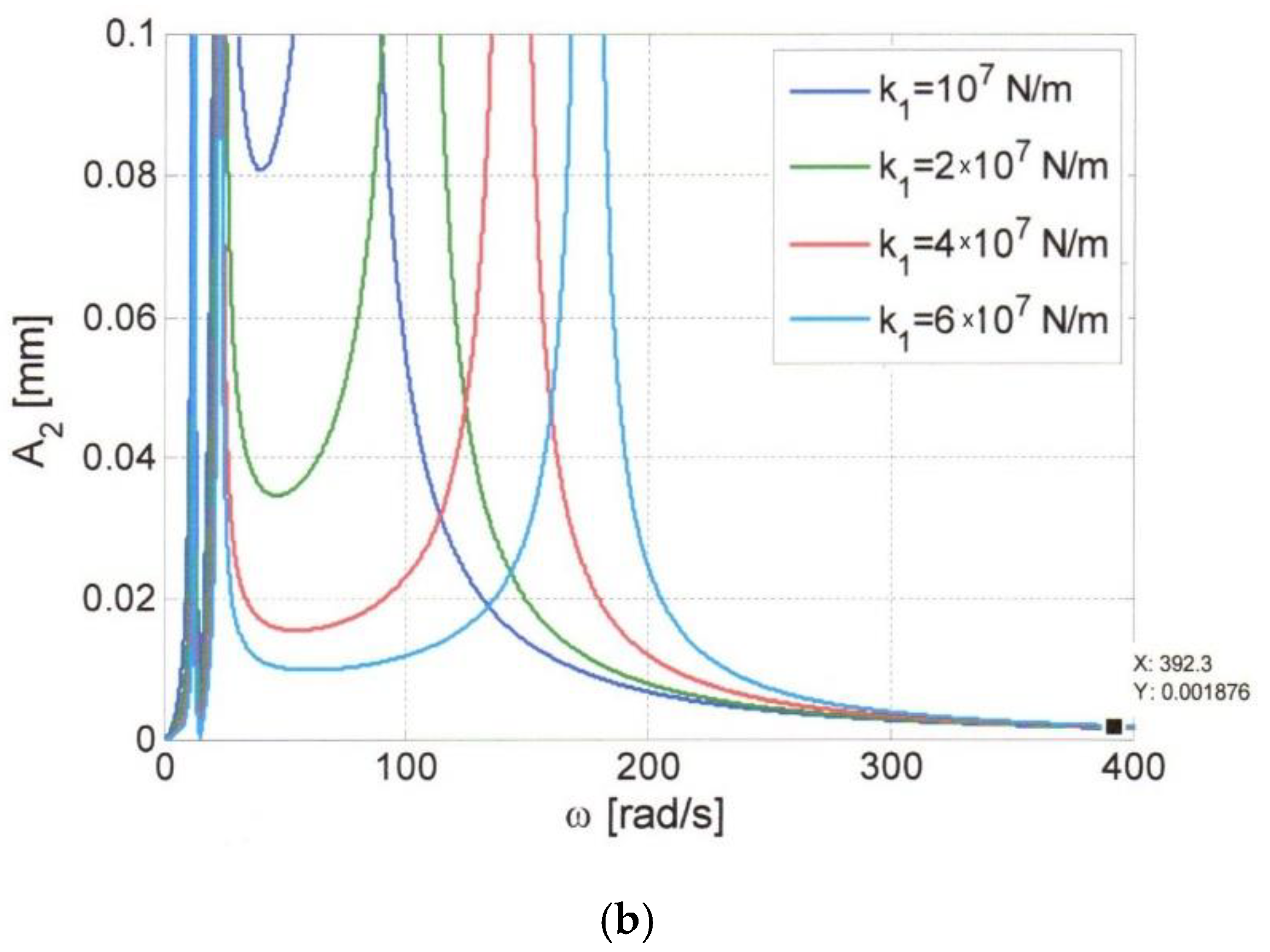
For the variation of ω in the range of values (0 ÷ 400) rad/s, the response curves of amplitudes A1(ω), A2(ω), and A3(ω) were drawn and represented in Figure 2, Figure 3 and Figure 4 for four discrete values of rigidity k1. Thus, three own pulses emerge of which the first two at the values rad/s, rad/s, are common and constant for the four values of rigidity N/m; the last value of the own pulse is different according to rigidity k1. In this case, for kj, j = 1, 2, 3, we have N/m, , N/m, rad/s, N/m, rad/s, and N/m, rad/s. It can be found that in the post-resonance regime for , amplitude A1 tends asymptomatically toward a constant value and stable motion at the value A1 = 1.245 mm, and amplitudes A2 and A3 tend toward very small values, of the order 1.87 × 10⁻³ mm, respectively, 3 × 10⁻⁷ rad.
In order to determine the resonance pulses to ensure a post-resonance regime, only the significant linear elastic case was considered, obviously with the neglect of the viscous effects.
The low numerical values of amplitudes A2 and A3 in post-resonance highlight the fact that the forced vibrations transmitted from body C1 to body C2 are negligible.
The amplitude variation curves in Figure 2, Figure 3 and Figure 4 were numerically elevated for the previously specified parametric data for a towed vibrating roller, with a hydrostatic system for continuously changing the excitation pulsation (i.e., the angular velocity of the eccentric mass of the vibrator). Thus, the resonance pulses were measured for each case, with an accuracy of ±5 Hz compared to the numerically obtained value. A Bosch hydrostatic control system and a Bruel & Kjaer vibration measurement system were used.
4. Conclusions
The structural assembly of a vibrating roller can be modeled as a system of two rigid bodies with linear elastic connections so that two contradictory desiderata can be achieved simultaneously, namely: achieving technological vibrations for body C1 (vibrating roller) and the significant reduction of the vibrations transmitted to body C2 (machine chassis) in the control cabin was assembled with the working space for the operating mechanic and the drive unit.
In this context, the modeling of the multi-body system was conducted taking into account the inertial characteristics in direct correlation with the possible and significant movements of the two rigid bodies. Thus, the vertical translational motion of body C1 of mass m1 is characterized by a coordinate or a single dynamic degree of freedom that describes the vertical instantaneous displacement.
The motion of the C2 body is characterized by two degrees of dynamic freedom defined by the x and φ coordinates. They describe the instantaneous vertical translational motion and respectively, the instantaneous angular rotational motion around the horizontal axis passing through the center of gravity of body C2. In this case, the multibody system is characterized by three degrees of dynamic freedom noted with x1, x, and φ.
As a result of the dynamic study developed in the paper, based on the numerical analysis and the experimental results obtained on five categories of equipment, the presented model faithfully describes the dynamic behavior of the tested equipment. In this context, the following conclusions can be drawn.
(a) The dynamic model of the multibody system with elastic connections is characterized by the inertia matrix M and by the rigidity matrix K, both symmetrical in relation to the main diagonal;
(b) The elements of inertial coupling and of elastic coupling and are found in the differential equations of motion (23) with significant effects on the equation of own pulses (27) and of amplitudes A1, A2, A3 as a dynamic response to the harmonic excitation .
(c) The numerical and experimental analysis on a vibrating roller equipment, with mass, elastic and excitation data, for the evaluated case study, provides the following conclusions:
- -
- the first two own pulses with relatively low values rad/s rad/s were influenced by the fact that the inertial effect is large enough and rigidity of the elastic connection system between bodies C1 and C2 is low enough for good post-resonance vibration isolation at ;
- -
- the last own pulse , is mainly influenced by rigidity of the compaction soil. Thus, for four distinct values of , which correspond to successive passages on the same layer of road structure, in the compaction process, there emerged four distinct values of the own pulses (resonance) , in ascending order, as follows: , rad/s, rad/s, rad/s [12].
(d) The family of curves for amplitudes A1, A2, and A3 represented in Figure 2, Figure 3 and Figure 4 highlights the fact that in the post-resonance regime for ω > ωn3, amplitude A1 of the technological vibrations is constant and stable for rad/s, and amplitudes A2 and A3 tend toward small values, assuring the favorable effect of dynamic insulation for body C2.
(e) The analytical relations (26), (27), and (28) can be used for the parametric optimization of the dynamic response, as follows:
- -
- amplitude A1 of the technological vibrations, which must be constant and stable at the excitation pulse ω, must meet the post-resonance operating condition ω > 1.5 ωn3. Practically, it is recommended that ω = 2ωn3 to achieve the technological requirements of efficient compaction;
- -
- amplitudes A2 and A3 of body C2 must have low values so that the degree of isolation of the vibrations transmitted from the body C1 to be ; and
- -
- the first two own pulses or resonance circular frequencies must be within the range (10 ÷ 60) rad/s, so that the influence of the two resonance zones for ω = ωn1 and ω = ωn2 becomes negligible for stable optimal operation [13].
Given the above, the analytical approach of the dynamic behavior of multibody systems with effective applications for vibratory rollers for compacting road structures can be useful in the stage of establishing technical design solutions as well as in the parametric optimization stage.
This can be achieved by adjustments and tuning that can be made during the working process such as the discrete change in steps, the static moment m0r, and/or the continuous modification of the excitation pulse ω that can be achieved with the hydrostatic actuation of the vibrator [14].
Funding
This research received no external funding.
Conflicts of Interest
The author declare no conflict of interest.
References
- Bratu, P.; Dobrescu, C.F. Dynamic Response of Zener-Modelled Linearly Viscoelastic Systems under Harmonic Excitation. Symmetry 2019, 11, 1050. [Google Scholar] [CrossRef] [Green Version]
- Dobrescu, C.F. The Zener rheological viscoelastic modelling of the dynamic compaction of the ecologically stabilized soils. Acta Tech. Napoc. 2019, 62, 281–286. [Google Scholar]
- Tonciu, O.; Dobrescu, C.F. Optimal dynamic regimes of vibration compaction equipment. Acta Tech. Napoc. 2020, 63, 101–106. [Google Scholar]
- Shabana, A.A. Dynamics of Multibody Systems; Cambridge University Press: Cambridge, UK, 2014. [Google Scholar]
- Bratu, P. Dynamique des compacteurs autopropulses avec deux rouleaux vibrateurs. Rev. Roum. Sci. Tech. Mec. Appl. 1988, 33, 349–366. [Google Scholar]
- Pandrea, N.; Stănescu, N.-D. Dynamics of the Rigid Solid with General Constrains by a Multibody Approach; John Wiley & Sons: Hoboken, NJ, USA, 2016. [Google Scholar]
- Bratu, P. Establishing the equations of motion for the rigid with elastic connections. Studies and researches of applied mechanics, SCMA, Romanian Academy, 1990. Volume 50, no. 6. Available online: https://books.google.ro/books?id=ejEeAQAAMAAJ&q (accessed on 28 September 2020).
- Bratu, P. Evaluation of quality dynamic performances in case of vibrating rollers used for road works. In Proceedings of the SISOM 2007 and Homagial Session of the Commission of Acoustics, Bucharest, Romania, 29–31 May 2007, 1st ed.; Research Institute for Construction Equipment and Technology ICECON SA: Bucharest, Romania, 2008; pp. 91–104. [Google Scholar]
- Schiehlen, W. Computational dynamics: Theory and applications of multibody systems. Eur. J. Mech. A Solids 2006, 25, 566–594. [Google Scholar] [CrossRef] [Green Version]
- Huston, R.L. Multibody dynamics—Modeling and analysis methods. Appl. Mech. Rev. 1991, 4, 109–117. [Google Scholar] [CrossRef]
- Wittenburg, J. Dynamics of Multibody Systems; Springer: Berlin/Heidelberg, Germany, 2007. [Google Scholar]
- Dobrescu, C.F. Analysis of the dynamic regime of forced vibrations in the dynamic compacting process with vibrating roller. Acta Tech. Napoc. Appl. Math. Mech. Eng. 2019, 62, 1. [Google Scholar]
- Dobrescu, C.F. Highlighting the Change of the Dynamic Response to Discrete Variation of Soil Stiffness in the Process of Dynamic Compaction with Roller Compactors Based on Linear Rheological Modelling. Appl. Mech. Mater 2015, 801, 242–248. [Google Scholar] [CrossRef]
- Dobrescu, C.F.; Brăguţă, E. Optimization of Vibro-Compaction Technological Process Considering Rheological Properties. In Proceedings of the Acoustics and Vibration of Mechanical Structures—AVMS-2017: 14th AVMS Conference, Timisoara, Romania, 25–26 May 2017; Herisanu, N., Marinca, V., Eds.; Springer: Cham, Switzerland, 2018; pp. 287–293. [Google Scholar]
Figure 1.
Dynamic multibody model with linear elastic connections.

Figure 2.
Family of curves for amplitude A1. (a) Normal representation. (b) Enlarged scale representation.
Figure 2.
Family of curves for amplitude A1. (a) Normal representation. (b) Enlarged scale representation.

Figure 3.
Family of curves for amplitude A2. (a) Normal representation. (b) Enlarged scale representation.
Figure 3.
Family of curves for amplitude A2. (a) Normal representation. (b) Enlarged scale representation.


Figure 4.
Family of curves for amplitude A3. (a) Normal representation. (b) Enlarged scale representation.
Figure 4.
Family of curves for amplitude A3. (a) Normal representation. (b) Enlarged scale representation.


© 2020 by the author. Licensee MDPI, Basel, Switzerland. This article is an open access article distributed under the terms and conditions of the Creative Commons Attribution (CC BY) license (http://creativecommons.org/licenses/by/4.0/).
Share and Cite
MDPI and ACS Style
Bratu, P. Multibody System with Elastic Connections for Dynamic Modeling of Compactor Vibratory Rollers. Symmetry 2020, 12, 1617. https://doi.org/10.3390/sym12101617
AMA Style
Bratu P. Multibody System with Elastic Connections for Dynamic Modeling of Compactor Vibratory Rollers. Symmetry. 2020; 12(10):1617. https://doi.org/10.3390/sym12101617
Chicago/Turabian StyleBratu, Polidor. 2020. "Multibody System with Elastic Connections for Dynamic Modeling of Compactor Vibratory Rollers" Symmetry 12, no. 10: 1617. https://doi.org/10.3390/sym12101617
Note that from the first issue of 2016, this journal uses article numbers instead of page numbers. See further details here.