Parametric Jensen-Shannon Statistical Complexity and Its Applications on Full-Scale Compartment Fire Data

Abstract

The order/disorder characteristics of a compartment fire are researched based on experimental data. From our analysis performed by new, pioneering methods, we claim that the parametric Jensen-Shannon complexity can be successfully used to detect unusual data, and that one can use it also as a means to perform relevant analysis of fire experiments. Thoroughly comparing the performance of different algorithms (known as permutation entropy and two-length permutation entropy) to extract the probability distribution is an essential step. We discuss some of the theoretical assumptions behind each step and stress that the role of the parameter is to fine-tune the results of the Jensen-Shannon statistical complexity. Note that the Jensen-Shannon statistical complexity is symmetric, while its parametric version displays a symmetric duality due to the a priori probabilities used.

1. Introduction

We aim to perform a local entropic analysis of the evolution of the temperature during a full-scale fire experiment and seek a straightforward, general, and process-based model of the compartment fire. We propose a new statistical complexity and compare known algorithms dedicated to the extraction of the underlying probabilities, checking their suitability to point out the abnormal values and structure of the experimental time series. For recent research on the fire phenomena performed using entropic tools, see Takagi, Gotoda, Tokuda and Miyano [1] and Murayama, Kaku, Funatsu, and Gotoda [2].

The experimental data was collected during a full-scale fire experiment conducted at the Fire Officers Faculty in Bucharest. We briefly include here the description of the experimental setup (Materials and Methods). Details can be found in [3].

The experiment has been carried out using a container (single-room compartment) having the following dimensions: 12 m × 2.2 m × 2.6 m. A single ventilation opening was available, namely the front door of the container, which remained open during the experiment. Parts of the walls and the ceiling of the container were furnished with oriented strand boards (OSB). The fire source has been a wooden crib made of 36 pieces of wood strips 2.5 cm × 2.5 cm × 30 cm, on which has been poured 500 mL ethanol shortly before ignition. The fire bed was situated in a corner of the compartment, at 1.2 m below the ceiling. The measurement devices consisted of six built-in K-type thermocouples, which were fixed at key locations (see Figure 1) and connected to a data acquisition logger. Flames were observed to impinge on the ceiling and exit through the opening, and we also noted the ignition of crumpled newspaper and stages of fire development that are known as indicators of flashover.

In Section 2, we present the theoretical background and briefly summarize the approaches that are used to model fire.

Section 3 is dedicated to the results regarding the analysis of the collected raw data.

2. Theoretical Background and Remarks

2.1. Entropy and Statistical Complexity

The natural logarithm is used below, as elsewhere in this paper.

Shannon’s entropy [4] is defined as $\mathrm{H}\left(\mathrm{P}\right)=-{{\displaystyle \sum }}_{\mathrm{i}=1}^{\mathrm{n}}{\mathrm{p}}_{\mathrm{i}}{\mathrm{logp}}_{\mathrm{i}}$, where $\mathrm{P}=\left({\mathrm{p}}_1,\dots ,{\mathrm{p}}_{\mathrm{n}}\right)$ is a finite probability distribution. It is nonnegative and its maximum value is $\mathrm{H}\left(\mathrm{U}\right)=\mathrm{logn}$, where $\mathrm{U}=\left(\frac{1}{\mathrm{n}},\dots ,\frac{1}{\mathrm{n}}\right).$ Throughout the paper, we use the convention $0·\log 0=0$.

The Kullback-Leibler divergence [5] is defined by

$$\mathrm{D}\left(\mathrm{P}\Vert \mathrm{R}\right)={\displaystyle \sum }_{\mathrm{i}=1}^{\mathrm{n}}{\mathrm{p}}_{\mathrm{i}}(\log {\mathrm{p}}_{\mathrm{i}}-\log {\mathrm{r}}_{\mathrm{i}})$$

(1)

where $\mathrm{P}=\left({\mathrm{p}}_1,\dots ,{\mathrm{p}}_{\mathrm{n}}\right)$ and $\mathrm{R}=\left({\mathrm{r}}_1,\dots ,{\mathrm{r}}_{\mathrm{n}}\right)$ are probability distributions. It is nonnegative and it vanishes for $\mathrm{P}=\mathrm{R}$.

If the value 0 appears in probability distributions $\mathrm{P}=\left({\mathrm{p}}_1,\dots ,{\mathrm{p}}_{\mathrm{n}}\right)$ and $\mathrm{R}=\left({\mathrm{r}}_1,\dots ,{\mathrm{r}}_{\mathrm{n}}\right)$, it must appear in the same positions for the sake of significance. Otherwise, one usually consider the conventions $0\log \frac{0}{\mathrm{b}}=0$ for $\mathrm{b}\ge 0$ and $\mathrm{a}\log \frac{\mathrm{a}}{0}=\infty$ for $\mathrm{a}>0$. We remark that these are strong limitations and such conditions rarely occur in practice.

To overcome this issue, the following divergence, well-defined, is used in the literature.

The Jensen-Shannon divergence (see [6,7]) is given by

$$\mathrm{JS}\left(\mathrm{P}\Vert \mathrm{R}\right)=\frac{1}{2}\mathrm{D}\left(\mathrm{P}\Vert \frac{\mathrm{P}+\mathrm{R}}{2}\right)+\frac{1}{2}\mathrm{D}\left(\mathrm{R}\Vert \frac{\mathrm{P}+\mathrm{R}}{2}\right)=\mathrm{H}\left(\frac{\mathrm{P}+\mathrm{R}}{2}\right)-\frac{\mathrm{H}\left(\mathrm{P}\right)+\mathrm{H}\left(\mathrm{R}\right)}{2}.$$

(2)

The disequilibrium-based statistical complexity (LMC statistical complexity) introduced in 1995 by López-Ruiz, Mancini, and Calbet in [8] is defined as $\mathrm{C}\left(\mathrm{P}\right)=\mathrm{D}\left(\mathrm{P}\right)\frac{\mathrm{H}\left(\mathrm{P}\right)}{\log \mathrm{n}},$ where $\mathrm{D}\left(\mathrm{P}\right)$, which is interpreted as disequilibrium, is the quadratic distance $\mathrm{D}\left(\mathrm{P}\right)={{\displaystyle \sum }}_{\mathrm{i}=1}^{\mathrm{n}}{({\mathrm{p}}_{\mathrm{i}}-\frac{1}{\mathrm{n}})}^2$.

Interpreted as entropic non-triviality (in Lamberti et al. [9] and Zunino et al. [10]), the Jensen-Shannon statistical complexity is defined by ${\mathrm{C}}^{\left(\mathrm{JS}\right)}\left(\mathrm{P}\right)={\mathrm{Q}}_{\left(\mathrm{JS}\right)}\left(\mathrm{P}\right)\frac{\mathrm{H}\left(\mathrm{P}\right)}{\log \mathrm{n}},$ where the disequilibrium ${\mathrm{Q}}_{\left(\mathrm{JS}\right)}\left(\mathrm{P}\right)$ is ${\mathrm{Q}}_{\left(\mathrm{JS}\right)}\left(\mathrm{P}\right)=\mathrm{k}·\mathrm{JS}\left(\mathrm{P}\Vert \mathrm{U}\right)$. Here, $\mathrm{k}={({\max }_{\mathrm{P}}\mathrm{JS}\left(\mathrm{P}\Vert \mathrm{U}\right))}^{-1}$ is the normalizing constant and $\mathrm{U}=\left(\frac{1}{\mathrm{n}},\dots ,\frac{1}{\mathrm{n}}\right).$ Therefore, we have $0\le {\mathrm{C}}^{\left(\mathrm{JS}\right)}\left(\mathrm{P}\right)\le 1$.

For the convenience of the interested reader, we include the following method to determine the normalizing constant (a result stated for computational purposes, without proof, in [9]).

Proposition 1.

Using the above notation, for the computation of the normalizing constant,$\mathrm{k}={({\max }_{\mathrm{P}}\mathrm{JS}\left(\mathrm{P}\Vert \mathrm{U}\right))}^{-1}$, the maximum is attained for$\mathrm{P}$such that there exists$\mathrm{i},{\mathrm{p}}_{\mathrm{i}}=1$.

It holds that$\mathrm{k}={\left(\log 2-\frac{1}{2}\log \frac{\mathrm{n}+1}{\mathrm{n}}-\frac{\log \left(\mathrm{n}+1\right)}{2\mathrm{n}}\right)}^{-1}$.

Proof. 

We have the following calculations:

$$\mathrm{JS}\left(\mathrm{P}\Vert \mathrm{U}\right)=\mathrm{H}\left(\frac{\mathrm{P}+\mathrm{U}}{2}\right)-\frac{\mathrm{H}\left(\mathrm{P}\right)+\mathrm{H}\left(\mathrm{U}\right)}{2}=\frac{1}{2}{\displaystyle \sum }_{\mathrm{i}=1}^{\mathrm{n}}{\mathrm{p}}_{\mathrm{i}}\log {\mathrm{p}}_{\mathrm{i}}-\frac{1}{2}\log \mathrm{n}-{\displaystyle \sum }_{\mathrm{i}=1}^{\mathrm{n}}\left(\frac{{\mathrm{p}}_{\mathrm{i}}}{2}+\frac{1}{2\mathrm{n}}\right)\log \left(\frac{{\mathrm{p}}_{\mathrm{i}}}{2}+\frac{1}{2\mathrm{n}}\right).$$

(3)

$$\frac{\partial \mathrm{JS}\left(\mathrm{P}\Vert \mathrm{U}\right)}{\partial {\mathrm{p}}_{\mathrm{i}}}=\frac{1}{2}\log {\mathrm{p}}_{\mathrm{i}}+\frac{1}{2}-\frac{1}{2}\log \left(\frac{{\mathrm{p}}_{\mathrm{i}}}{2}+\frac{1}{2\mathrm{n}}\right)-\frac{1}{2}=\frac{1}{2}\log {\mathrm{p}}_{\mathrm{i}}-\frac{1}{2}\log \left(\frac{{\mathrm{p}}_{\mathrm{i}}}{2}+\frac{1}{2\mathrm{n}}\right).$$

(4)

$$\frac{{\partial }^2\mathrm{JS}\left(\mathrm{P}\Vert \mathrm{U}\right)}{\partial {\mathrm{p}\mathrm{i}}^2}=\frac{1}{2{\mathrm{p}}_{\mathrm{i}}}-\frac{1}{4\left(\frac{{\mathrm{p}}_{\mathrm{i}}}{2}+\frac{1}{2\mathrm{n}}\right)}=\frac{1}{2{\mathrm{p}}_{\mathrm{i}}}-\frac{1}{2{\mathrm{p}}_{\mathrm{i}}+\frac{2}{\mathrm{n}}}>0,\frac{{\partial }^2\mathrm{JS}\left(\mathrm{P}\Vert \mathrm{U}\right)}{\partial {\mathrm{p}}_{\mathrm{i}}\partial {\mathrm{p}}_{\mathrm{j}}}=0.$$

(5)

So, the Hessian of $\mathrm{JS}\left(\mathrm{P}\Vert \mathrm{U}\right)$ is everywhere positive definite, whence $\mathrm{JS}\left(\mathrm{P}\Vert \mathrm{U}\right)$ is (strictly) convex on the open convex set $\left\{\left({\mathrm{p}}_1,\dots ,{\mathrm{p}}_{\mathrm{n}}\right):0<{\mathrm{p}}_{\mathrm{i}}<1\mathrm{for}\mathrm{all}\mathrm{i},{{\displaystyle \sum }}_{\mathrm{i}=1}^{\mathrm{n}}{\mathrm{p}}_{\mathrm{i}}=1\right\}$. Therefore, $\mathrm{JS}\left(\mathrm{P}\Vert \mathrm{U}\right)$ cannot have a maximum inside (otherwise, it would be constant), and the points of maximum must lie on the boundary. See Theorem 3.10.10 in [11] (p. 171). Such points exist, because $\mathrm{JS}\left(\mathrm{P}\Vert \mathrm{U}\right)$ is continuous on the compact set $\mathsf{\Delta }=\left\{\left({\mathrm{p}}_1,\dots ,{\mathrm{p}}_{\mathrm{n}}\right):0\le {\mathrm{p}}_{\mathrm{i}}\le 1\mathrm{for}\mathrm{all}\mathrm{i},{{\displaystyle \sum }}_{\mathrm{i}=1}^{\mathrm{n}}{\mathrm{p}}_{\mathrm{i}}=1\right\}$. The function $\mathrm{JS}\left(\mathrm{P}\Vert \mathrm{U}\right)$ is continuous and convex on the compact convex set $\mathsf{\Delta }$, so its maximum lies on the set of vertices of $\mathsf{\Delta }$ (${\mathrm{where}\mathrm{p}}_{\mathrm{i}}=1\mathrm{for}\mathrm{one}\mathrm{i}$). See Theorem 3.10.11 in [11] (p. 171). Since $\mathrm{JS}\left(\mathrm{P}\Vert \mathrm{U}\right)$ does not depend on the order of the components of $\mathrm{P}$, the maximum value is attained at all vertices, so it can be straightforwardly computed by setting $\mathrm{P}=\left(1,0,\dots ,0\right)$. □

Remark 1.

Note that the maximal value of$\mathrm{JS}\left(\mathrm{P}\Vert \mathrm{U}\right)$is$\log 2-\frac{1}{2}\log \frac{\mathrm{n}+1}{\mathrm{n}}-\frac{\log \left(\mathrm{n}+1\right)}{2\mathrm{n}}\nearrow \log 2,$as$\mathrm{n}\to \infty .$Since$\mathrm{JS}\left(\mathrm{P}\Vert \mathrm{U}\right)$is bounded from above by$\log 2$, independently of$\mathrm{n}$, the normalization of$\mathrm{JS}\left(\mathrm{P}\Vert \mathrm{U}\right)$in the definition of the Jensen-Shannon complexity does not seem to be relevant, and one could simply consider$\mathrm{JS}\left(\mathrm{P}\Vert \mathrm{U}\right)\frac{\mathrm{H}\left(\mathrm{P}\right)}{\log \mathrm{n}}$.

Let$\mathsf{\lambda }\in \left[0,1\right]$. The parametric Jensen-Shannon divergence (see for instance, [6]) is given by

$$\begin{array}{c}\hfill {\mathrm{JS}}_{\mathsf{\lambda }}\left(\mathrm{P}\Vert \mathrm{R}\right)=\left(1-\mathsf{\lambda }\right)\mathrm{D}\left(\mathrm{P}\Vert \left(1-\mathsf{\lambda }\right)\mathrm{P}+\mathsf{\lambda }\mathrm{R}\right)+\mathsf{\lambda }\mathrm{D}\left(\mathrm{R}\Vert \left(1-\mathsf{\lambda }\right)\mathrm{P}+\mathsf{\lambda }\mathrm{R}\right)\\ \hfill =\mathrm{H}\left(\left(1-\mathsf{\lambda }\right)\mathrm{P}+\mathsf{\lambda }\mathrm{R}\right)-\left(\left(1-\mathsf{\lambda }\right)\mathrm{H}\left(\mathrm{P}\right)+\mathsf{\lambda }\mathrm{H}\left(\mathrm{R}\right)\right).\end{array}$$

(6)

It is positive and it vanishes for$\mathrm{P}=\mathrm{R}$or$\mathsf{\lambda }=0\mathrm{or}1$. See also Figure 2.

The values$1-\mathsf{\lambda }$and$\mathsf{\lambda }$are interpreted as a priori probabilities. Note that${\mathrm{JS}}_{\mathsf{\lambda }}\left(\mathrm{P}\Vert \mathrm{R}\right)={\mathrm{JS}}_{1-\mathsf{\lambda }}\left(\mathrm{R}\Vert \mathrm{P}\right)$and${\mathrm{JS}}_{\mathsf{\lambda }}$is not symmetric, unless$\mathsf{\lambda }=0.5$.

Mutatis mutandis, from Donald’s identity (Lemma 2.12 in [12]), one has

$${\mathrm{JS}}_{\mathsf{\lambda }}\left(\mathrm{P}\Vert \mathrm{R}\right)+\mathrm{D}\left(\left(1-\mathsf{\lambda }\right)\mathrm{P}+\mathsf{\lambda }\mathrm{R}\Vert \mathrm{Q}\right)=\left(1-\mathsf{\lambda }\right)\mathrm{D}\left(\mathrm{P}\Vert \mathrm{Q}\right)+\mathsf{\lambda }\mathrm{D}\left(\mathrm{R}\Vert \mathrm{Q}\right)$$

(7)

for an arbitrarily fixed $\mathsf{\lambda }\in \left[0,1\right]$. One needs only straightforward computation to check that it holds. Therefore,

$$\begin{array}{c}{\mathrm{JS}}_{\mathsf{\lambda }}\left(\mathrm{P}\Vert \mathrm{R}\right)=\min \{\left(1-\mathsf{\lambda }\right)\mathrm{D}\left(\mathrm{P}\Vert \mathrm{Q}\right)+\mathsf{\lambda }\mathrm{D}\left(\mathrm{R}\Vert \mathrm{Q}\right):\mathrm{Q}=\hfill \\ \left({\mathrm{q}}_1,\dots ,{\mathrm{q}}_{\mathrm{n}}\right)\mathrm{is}\mathrm{a}\mathrm{finite}\mathrm{probability}\mathrm{distribution}\}.\hfill \end{array}$$

(8)

We introduce the parametric Jensen-Shannon statistical complexity as

$${\mathrm{C}}_{\mathsf{\lambda }}^{\left(\mathrm{JS}\right)}\left(\mathrm{P}\right)\equiv {\mathrm{JS}}_{\mathsf{\lambda }}\left(\mathrm{P}\Vert \mathrm{U}\right)\frac{\mathrm{H}\left(\mathrm{P}\right)}{\log \mathrm{n}}.$$

(9)

As in the case of the complexities $\mathrm{C}\left(\mathrm{P}\right),{\mathrm{C}}^{\left(\mathrm{JS}\right)}\left(\mathrm{P}\right),$ the new ones,${\mathrm{C}}_{\mathsf{\lambda }}^{\left(\mathrm{JS}\right)}\left(\mathrm{P}\right),$ would be zero (minimum complexity) for $\mathrm{P}=\mathrm{U}$ or if there exists $\mathrm{i}$ such that ${\mathrm{p}}_{\mathrm{i}}=1$. These two cases describe very different states of the system, both of which are extreme circumstances being considered simple, namely the states with respectively maximum and minimum entropy.

We do not need to normalize ${\mathrm{JS}}_{\mathsf{\lambda }}\left(\mathrm{P}\Vert \mathrm{U}\right)$ in the definition of the parametric Jensen-Shannon complexity (possibly one can feel more comfortable with its normalized version in other frameworks), but we stress that one can easily prove, following the same recipe as above, that its maximum value is attained for $\mathrm{P}$ such that there exists $\mathrm{i},{\mathrm{p}}_{\mathrm{i}}=1$.

Proposition 2.

Let$\mathsf{\lambda }\in \left[0,1\right]$. Using the above notation, it holds

$$\underset{\mathrm{P}}{\max }{\mathrm{JS}}_{\mathsf{\lambda }}\left(\mathrm{P}\Vert \mathrm{U}\right)=-\mathsf{\lambda }\log \mathsf{\lambda }-\left(1-\mathsf{\lambda }\right)\log \left(1-\mathsf{\lambda }\right)-\left(1-\mathsf{\lambda }\right)\log \left(1+\frac{\mathsf{\lambda }}{\left(1-\mathsf{\lambda }\right)\mathrm{n}}\right)-\frac{\mathsf{\lambda }}{\mathrm{n}}\log \frac{\left(1-\mathsf{\lambda }\right)\mathrm{n}+\mathsf{\lambda }}{\mathsf{\lambda }}.$$

(10)

Moreover, $\underset{\mathrm{P}}{\max }{\mathrm{JS}}_{\mathsf{\lambda }}\left(\mathrm{P}\Vert \mathrm{U}\right)\nearrow -\mathsf{\lambda }\log \mathsf{\lambda }-\left(1-\mathsf{\lambda }\right)\log \left(1-\mathsf{\lambda }\right)\le \log 2,$ as $\mathrm{n}\to \infty .$

Proof. 

We omit the computation of $\underset{\mathrm{P}}{\max }{\mathrm{JS}}_{\mathsf{\lambda }}\left(\mathrm{P}\Vert \mathrm{U}\right),$ which is straightforward.

To justify the monotonicity, it is enough to prove that $\mathrm{f}\left(\mathrm{x}\right)=\frac{\mathsf{\lambda }}{\mathrm{x}}\log \frac{\left(1\mathrm{g}\mathsf{\lambda }\right)\mathrm{x}+\mathsf{\lambda }}{\mathsf{\lambda }}$ is decreasing:

$${\mathrm{f}}^{\prime }\left(\mathrm{x}\right)=-\frac{\mathsf{\lambda }}{{\mathrm{x}}^2}\left[\frac{\mathsf{\lambda }}{\left(1-\mathsf{\lambda }\right)\mathrm{x}+\mathsf{\lambda }}-1-\log \frac{\mathsf{\lambda }}{\left(1-\mathsf{\lambda }\right)\mathrm{x}+\mathsf{\lambda }}\right]<0,\mathrm{for}\mathsf{\lambda }\in \left(0,1\right)\mathrm{and}\mathrm{x}>0.$$

(11)

Furthermore, it is obvious that $\left(1-\mathsf{\lambda }\right)\log \left(1+\frac{\mathsf{\lambda }}{\left(1-\mathsf{\lambda }\right)\mathrm{n}}\right)+\frac{\mathsf{\lambda }}{\mathrm{n}}\log \frac{\left(1-\mathsf{\lambda }\right)\mathrm{n}+\mathsf{\lambda }}{\mathsf{\lambda }}\to 0$.

The last inequality follows from Jensen’s inequality, which is applied to the concave logarithmic function.

Therefore, ${\mathrm{JS}}_{\mathsf{\lambda }}\left(\mathrm{P}\Vert \mathrm{U}\right)$ is bounded from above by $\log 2$, independently of $\mathrm{n}$. □

Remark 2.

We split this result into two inequalities (of independent interest), which can be proved by the same technique. Namely, it holds that

$$\underset{\mathrm{P}}{\max }\mathrm{D}\left(\mathrm{P}\Vert \left(1-\mathsf{\lambda }\right)\mathrm{P}+\mathsf{\lambda }\mathrm{U}\right)\nearrow -\log \left(1-\mathsf{\lambda }\right)$$

(12)

and

$$\underset{\mathrm{P}}{\max }\mathrm{D}\left(\mathrm{U}\Vert \left(1-\mathsf{\lambda }\right)\mathrm{P}+\mathsf{\lambda }\mathrm{U}\right)\nearrow -\log \mathsf{\lambda },$$

(13)

as$\mathrm{n}\to \infty$.

Proposition 3.

Let$\mathsf{\lambda },\mathsf{\mu }\in \left[0,1\right]$. Using the above notation, the following inequality holds:

$$\min \left\{\frac{1-\mathsf{\lambda }}{1-\mathsf{\mu }},\frac{\mathsf{\lambda }}{\mathsf{\mu }}\right\}{\mathrm{JS}}_{\mathsf{\mu }}\left(\mathrm{P}\Vert \mathrm{R}\right)\le {\mathrm{JS}}_{\mathsf{\lambda }}\left(\mathrm{P}\Vert \mathrm{R}\right)\le \max \left\{\frac{1-\mathsf{\lambda }}{1-\mathsf{\mu }},\frac{\mathsf{\lambda }}{\mathsf{\mu }}\right\}{\mathrm{JS}}_{\mathsf{\mu }}\left(\mathrm{P}\Vert \mathrm{R}\right)$$

(14)

where$\mathrm{P}=\left({\mathrm{p}}_1,\dots ,{\mathrm{p}}_{\mathrm{n}}\right)$and$\mathrm{R}=\left({\mathrm{r}}_1,\dots ,{\mathrm{r}}_{\mathrm{n}}\right)$are two finite probability distributions.

Proof. 

The result is a particular case of Theorem 3.2 from [13]. We include here an alternative proof for the sake of completeness.

It is known that the entropy $\mathrm{H}$ is concave; Hence, $\mathrm{H}\left(\left(1-\mathsf{\lambda }\right)\mathrm{P}+\mathsf{\lambda }\mathrm{R}\right)\ge \left(1-\mathsf{\lambda }\right)\mathrm{H}\left(\mathrm{P}\right)+\mathsf{\lambda }\mathrm{H}\left(\mathrm{R}\right)$. We prove that

$$\min \left\{\frac{1-\mathsf{\lambda }}{1-\mathsf{\mu }},\frac{\mathsf{\lambda }}{\mathsf{\mu }}\right\}\left[\mathrm{H}\left(\left(1-\mathsf{\mu }\right)\mathrm{P}+\mathsf{\mu }\mathrm{R}\right)-\left(1-\mathsf{\mu }\right)\mathrm{H}\left(\mathrm{P}\right)-\mathsf{\mu }\mathrm{H}\left(\mathrm{R}\right)\right]\le$$

(15)

$$\mathrm{H}\left(\left(1-\mathsf{\lambda }\right)\mathrm{P}+\mathsf{\lambda }\mathrm{R}\right)-\left(1-\mathsf{\lambda }\right)\mathrm{H}\left(\mathrm{P}\right)-\mathsf{\lambda }\mathrm{H}\left(\mathrm{R}\right)\le$$

(16)

$$\max \left\{\frac{1-\mathsf{\lambda }}{1-\mathsf{\mu }},\frac{\mathsf{\lambda }}{\mathsf{\mu }}\right\}\left[\mathrm{H}\left(\left(1-\mathsf{\mu }\right)\mathrm{P}+\mathsf{\mu }\mathrm{R}\right)-\left(1-\mathsf{\mu }\right)\mathrm{H}\left(\mathrm{P}\right)-\mathsf{\mu }\mathrm{H}\left(\mathrm{R}\right)\right].$$

(17)

We consider $0\le \frac{1-\mathsf{\lambda }}{1-\mathsf{\mu }}\le \frac{\mathsf{\lambda }}{\mathsf{\mu }}$, so $\mathsf{\lambda }\ge \mathsf{\mu },$ which implies, by the concavity of $\mathrm{H}$, that

$$\left(1-\mathsf{\lambda }\right)\mathrm{H}\left(\mathrm{P}\right)+\mathsf{\lambda }\mathrm{H}\left(\mathrm{R}\right)+\min \left\{\frac{1-\mathsf{\lambda }}{1-\mathsf{\mu }},\frac{\mathsf{\lambda }}{\mathsf{\mu }}\right\}\left[\mathrm{H}\left(\left(1-\mathsf{\mu }\right)\mathrm{P}+\mathsf{\mu }\mathrm{R}\right)-\left(1-\mathsf{\mu }\right)\mathrm{H}\left(\mathrm{P}\right)-\mathsf{\mu }\mathrm{H}\left(\mathrm{R}\right)\right]=$$

(18)

$$\left(1-\mathsf{\lambda }\right)\mathrm{H}\left(\mathrm{P}\right)+\mathsf{\lambda }\mathrm{H}\left(\mathrm{R}\right)+\frac{1-\mathsf{\lambda }}{1-\mathsf{\mu }}\left[\mathrm{H}\left(\left(1-\mathsf{\mu }\right)\mathrm{P}+\mathsf{\mu }\mathrm{R}\right)-\left(1-\mathsf{\mu }\right)\mathrm{H}\left(\mathrm{P}\right)-\mathsf{\mu }\mathrm{H}\left(\mathrm{R}\right)\right]=$$

(19)

$$\frac{\mathsf{\lambda }-\mathsf{\mu }}{1-\mathsf{\mu }}\mathrm{H}\left(\mathrm{R}\right)+\frac{1-\mathsf{\lambda }}{1-\mathsf{\mu }}\mathrm{H}\left(\left(1-\mathsf{\mu }\right)\mathrm{P}+\mathsf{\mu }\mathrm{R}\right)\le \mathrm{H}\left(\frac{\mathsf{\lambda }-\mathsf{\mu }}{1-\mathsf{\mu }}\mathrm{R}+\frac{1-\mathsf{\lambda }}{1-\mathsf{\mu }}\left(\left(1-\mathsf{\mu }\right)\mathrm{P}+\mathsf{\mu }\mathrm{R}\right)\right)=$$

$$\mathrm{H}\left(\left(1-\mathsf{\lambda }\right)\mathrm{P}+\mathsf{\lambda }\mathrm{R}\right),$$

(20)

because it holds $\frac{\mathsf{\lambda }-\mathsf{\mu }}{1-\mathsf{\mu }}+\frac{1-\mathsf{\lambda }}{1-\mathsf{\mu }}=1$ and $\mathsf{\lambda }-\mathsf{\mu }\ge 0$.

For the second inequality, we have

$$\left(1-\mathsf{\lambda }\right)\mathrm{H}\left(\mathrm{P}\right)+\mathsf{\lambda }\mathrm{H}\left(\mathrm{R}\right)+\max \left\{\frac{1-\mathsf{\lambda }}{1-\mathsf{\mu }},\frac{\mathsf{\lambda }}{\mathsf{\mu }}\right\}\left[\mathrm{H}\left(\left(1-\mathsf{\mu }\right)\mathrm{P}+\mathsf{\mu }\mathrm{R}\right)-\left(1-\mathsf{\mu }\right)\mathrm{H}\left(\mathrm{P}\right)-\mathsf{\mu }\mathrm{H}\left(\mathrm{R}\right)\right]=$$

(21)

$$\left(1-\mathsf{\lambda }\right)\mathrm{H}\left(\mathrm{P}\right)+\mathsf{\lambda }\mathrm{H}\left(\mathrm{R}\right)+\frac{\mathsf{\lambda }}{\mathsf{\mu }}\left[\mathrm{H}\left(\left(1-\mathsf{\mu }\right)\mathrm{P}+\mathsf{\mu }\mathrm{R}\right)-\left(1-\mathsf{\mu }\right)\mathrm{H}\left(\mathrm{P}\right)-\mathsf{\mu }\mathrm{H}\left(\mathrm{R}\right)\right]=$$

$$-\frac{\mathsf{\lambda }-\mathsf{\mu }}{\mathsf{\mu }}\mathrm{H}\left(\mathrm{P}\right)+\frac{\mathsf{\lambda }}{\mathsf{\mu }}\mathrm{H}\left(\left(1-\mathsf{\mu }\right)\mathrm{P}+\mathsf{\mu }\mathrm{R}\right)\ge \mathrm{H}\left(\left(1-\mathsf{\lambda }\right)\mathrm{P}+\mathsf{\lambda }\mathrm{R}\right),$$

(22)

because it holds that $\frac{\mathsf{\lambda }}{\mathsf{\mu }}\mathrm{H}\left(\left(1-\mathsf{\mu }\right)\mathrm{P}+\mathsf{\mu }\mathrm{R}\right)\ge \mathrm{H}\left(\left(1-\mathsf{\lambda }\right)\mathrm{P}+\mathsf{\lambda }\mathrm{R}\right)+\frac{\mathsf{\lambda }-\mathsf{\mu }}{\mathsf{\mu }}\mathrm{H}\left(\mathrm{P}\right),$ which is equivalent to

$$\mathrm{H}\left(\left(1-\mathsf{\mu }\right)\mathrm{P}+\mathsf{\mu }\mathrm{R}\right)\ge \frac{\mathsf{\mu }}{\mathsf{\lambda }}\mathrm{H}\left(\left(1-\mathsf{\lambda }\right)\mathrm{P}+\mathsf{\lambda }\mathrm{R}\right)+\frac{\mathsf{\lambda }-\mathsf{\mu }}{\mathsf{\lambda }}\mathrm{H}\left(\mathrm{P}\right).$$

(23)

For $0\le \frac{\mathsf{\lambda }}{\mathsf{\mu }}\le \frac{1-\mathsf{\lambda }}{1-\mathsf{\mu }}$, the proof is similar. □

Remark 3.

For$\mathsf{\lambda }\in \left[0,1\right]$,$\mathsf{\mu }\in$(0,1), and$\mathrm{R}=\mathrm{U}$in Equation (1), then the following inequality holds:

$$\min \left\{\frac{1-\mathsf{\lambda }}{1-\mathsf{\mu }},\frac{\mathsf{\lambda }}{\mathsf{\mu }}\right\}{\mathrm{JS}}_{\mathsf{\mu }}\left(\mathrm{P}\Vert \mathrm{U}\right)\le {\mathrm{JS}}_{\mathsf{\lambda }}\left(\mathrm{P}\Vert \mathrm{U}\right)\le \max \left\{\frac{1-\mathsf{\lambda }}{1-\mathsf{\mu }},\frac{\mathsf{\lambda }}{\mathsf{\mu }}\right\}{\mathrm{JS}}_{\mathsf{\mu }}\left(\mathrm{P}\Vert \mathrm{U}\right).$$

(24)

For$\mathsf{\mu }=\frac{1}{2}$in Equation (3), we obtain:

$$2\min \left\{1-\mathsf{\lambda },\mathsf{\lambda }\right\}\mathrm{JS}\left(\mathrm{P}\Vert \mathrm{U}\right)\le {\mathrm{JS}}_{\mathsf{\lambda }}\left(\mathrm{P}\Vert \mathrm{U}\right)\le 2\max \left\{1-\mathsf{\lambda },\mathsf{\lambda }\right\}\mathrm{JS}\left(\mathrm{P}\Vert \mathrm{U}\right).$$

(25)

Multiplying by$\frac{\mathrm{H}\left(\mathrm{P}\right)}{\mathrm{logn}}$in Equation (4), we deduce the following inequality related to the parametric Jensen-Shannon statistical complexity:

$$2\mathrm{k}\min \left\{1-\mathsf{\lambda },\mathsf{\lambda }\right\}{\mathrm{C}}^{\left(\mathrm{JS}\right)}\left(\mathrm{P}\right)\le {\mathrm{C}}_{\mathsf{\lambda }}^{\left(\mathrm{JS}\right)}\left(\mathrm{P}\right)\le 2\mathrm{k}\max \left\{1-\mathsf{\lambda },\mathsf{\lambda }\right\}{\mathrm{C}}^{\left(\mathrm{JS}\right)}\left(\mathrm{P}\right),$$

(26)

where$\mathrm{k}=\log 2-\frac{1}{2}\log \frac{\mathrm{n}+1}{\mathrm{n}}-\frac{\log \left(\mathrm{n}+1\right)}{2\mathrm{n}}$.

2.2. Extraction of the Underlying Probability Distribution

The permutation entropy (PE) [14] quantifies randomness and the complexity of a time series based on the appearance of ordinal patterns, that is on comparisons of neighboring values of a time series. For other details on the PE algorithm applied to the present experimental data, see [3].

Let $\mathrm{T}=\left({\mathrm{t}}_1,\dots ,{\mathrm{t}}_{\mathrm{n}}\right)$ be a time series with distinct values.

Step 1. The increasing rearranging of the components of each $\mathrm{j}$-tuple $\left({\mathrm{t}}_{\mathrm{i}},\dots ,{\mathrm{t}}_{\mathrm{i}+\mathrm{j}-1}\right)$ as $\left({\mathrm{t}}_{\mathrm{i}+{\mathrm{r}}_1-1},\dots ,{\mathrm{t}}_{\mathrm{i}+{\mathrm{r}}_{\mathrm{j}}-1}\right)$ yields a unique permutation of order $\mathrm{j}$ denoted by $\mathsf{\pi }=\left({\mathrm{r}}_1,\dots ,{\mathrm{r}}_{\mathrm{j}}\right),$ which is an encoding pattern that describes the up-and-downs in the considered j-tuple.

Simple numerical examples may help clarify the concepts throughout this section.

Example 1.

For the five-tuple$\left(2.3,1,3.1,6.1,5.2\right)$, the corresponding permutation (encoding) is$\left(2,1,3,5,4\right).$

Step 2. The absolute frequency of this permutation (the number of $\mathrm{j}$-tuples which are associated to this permutation) is

$${\mathrm{k}}_{\mathsf{\pi }}\equiv \#\left\{\mathrm{i}:\mathrm{i}\le \mathrm{n}-\left(\mathrm{j}-1\right),\left({\mathrm{t}}_{\mathrm{i}},\dots ,{\mathrm{t}}_{\mathrm{i}+\mathrm{j}-1}\right)\mathrm{is}\mathrm{of}\mathrm{type}\mathsf{\pi }\right\}.$$

(27)

These values have the sum equal to the number of all the consecutive j-tuples; that is, $\mathrm{n}-\left(\mathrm{j}-1\right).$

Step 3. The permutation entropy of order $\mathrm{j}$ is defined as $\mathrm{PE}\left(\mathrm{j}\right)\equiv -{{\displaystyle \sum }}_{\mathsf{\pi }}{\mathrm{p}}_{\mathsf{\pi }}{\mathrm{logp}}_{\mathsf{\pi }}$, where ${\mathrm{p}}_{\mathsf{\pi }}=\frac{{\mathrm{k}}_{\mathsf{\pi }}}{\mathrm{n}-\left(\mathrm{j}-1\right)}$ is the relative frequency.

In [14], the measured values of the time series are considered distinct. The authors neglect equalities and propose to break them by adding small random perturbations (random noise) to the original series.

Another known approach is to rank the equalities according to their order of emergence (to rank the equalities with their sequential/chronological order, see for instance [15,16]). We use this method throughout the paper to compute $\mathrm{PE}\left(\mathrm{j}\right)$ for $\mathrm{j}$ = 3, 4, 5.

Applying the PE algorithm for experimental fire data, ${\mathrm{C}}_{\mathsf{\lambda }}^{\left(\mathrm{JS}\right)}\left(\mathrm{P}\right)$ cannot be zero. The number of the encoding patterns that occur is >1, and these patterns are not equiprobable: some patterns may be rare or locally forbidden (that is, one encounters such patterns at some thermocouples, but not in all six time series), as discussed in [3].

We briefly describe now the encoding steps in the TLPE algorithm (Two-Length Permutation Entropy algorithm) given by Watt and Politi in [17]; other details are provided in [3].

Step 1 given the $\mathrm{j}$-tuple $\mathrm{T}=\left({\mathrm{t}}_1,\dots ,{\mathrm{t}}_{\mathrm{j}}\right)$, we start encoding the last $\mathrm{k}$ ≤ $\mathrm{j}$ elements $\left({\mathrm{t}}_{\mathrm{j}-\mathrm{k}+1},\dots ,{\mathrm{t}}_{\mathrm{j}}\right)$ according to the ordinal position of each element; that is, every ${\mathrm{t}}_{\mathrm{s}}$ is replaced by a symbol which indicates the position occupied by ${\mathrm{t}}_{\mathrm{s}}$ within the increasing rearranging of the considered $\mathrm{k}$-tuple.

Next, we proceed by encoding each previous element ${\mathrm{t}}_{\mathrm{m}}$ up to $\mathrm{m}=1$ according to the symbol provided by Step 1 applied to the $\mathrm{k}$-tuple $\left({\mathrm{t}}_{\mathrm{m}},\dots ,{\mathrm{t}}_{\mathrm{m}+\mathrm{k}-1}\right)$.

Example 2.

Encoding obtained by the chronological ordering of equal values$\left(4.1,4.1,4.1,5,2.1\right)\to \left(1,1,2,3,1\right)$for$\mathrm{k}$= 3 and j = 5.

Step 2 and Step 3, they coincide with Step 2 and Step 3 in the PE algorithm above.

This algorithm leads, after computing the relative frequencies of the encoding sequences, to the two-length permutation entropy (TLPE $\left(\mathrm{k},\mathrm{j}\right)$).

Given the pair $\left(\mathrm{k},\mathrm{j}\right)$ of values, the number of symbolic (encoding) sequences of length $\mathrm{j}$ is $\mathrm{k}!{\mathrm{k}}^{\mathrm{j}-\mathrm{k}},$ which is a number that can be much smaller than j!, so this algorithm is faster, it involves a simplified computation, and sometimes it makes the results more relevant for big values of j.

We deal with the equal values by using the same method as for PE; that is, we consider them ordered chronologically.

In the next section, we apply the above techniques and observe their capability to discern the changes of the parametric Jensen-Shannon statistical complexity of the experimental data.

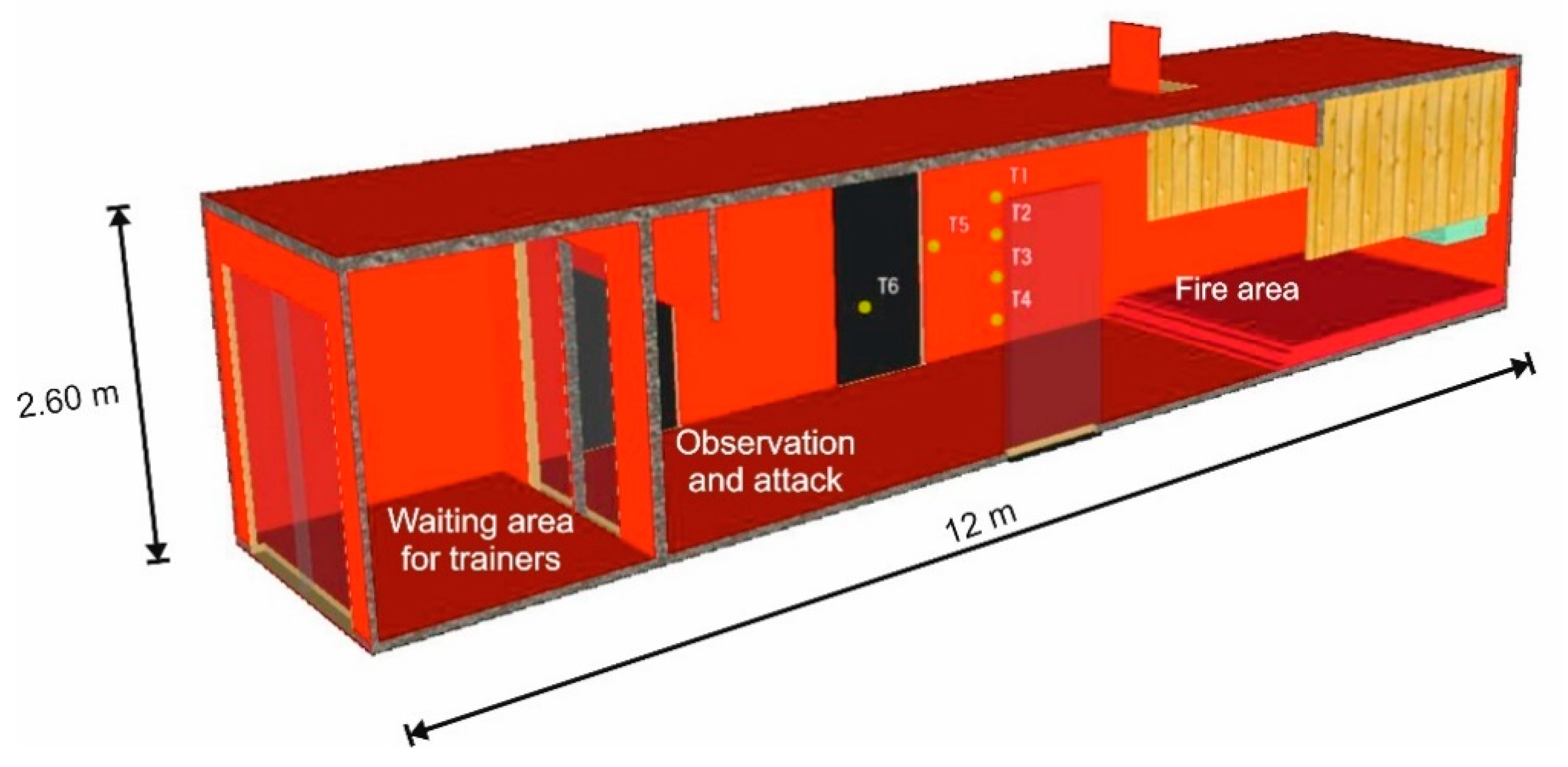
3. Raw Data Analysis

The raw data set under consideration consists of measured temperatures during a compartment fire: six thermocouples T1, …, T6 measure the temperatures every second during the experiment. Hence, we get six time series consisting of 3046 entries (data points), and we aim to a better understanding of these results by modeling the time series using information theory, and to assess the performance of the discussed statistical complexities.

We plot the parametric Jensen-Shannon statistical complexity against the parameter (for $\mathsf{\lambda }\in \left\{0,0.2,\dots ,1\right\}$). We notice the unusual plotting for the time series at T5, which is definitely not caused by the position of this thermocouple. The graph corresponding to the time series at T5 is far from the rest of the graphs for the other thermocouples; hence, smaller values were obtained for the statistical complexities, with no apparent experiment related or mathematical reason. See Figure 3, Figure 4, Figure 5, Figure 6 and Figure 7.

We conclude that the PE and TLPE algorithms can be successfully used to detect unusual data collected in fire experiments: different embedding dimensions and different algorithms used to determine the underlying probabilities provide the same conclusion, the hierarchy among the statistical complexities established for the thermocouples T1–T5 is the same, and T5 is always at a bigger distance from the rest of them. The position of the thermocouple T5 does not justify this big difference (see Figure 1). This also agrees with the smaller values provided at T5 by the LMC statistical complexity in Figure 8.

It is not clear in [9] why only the disequilibrium provided by $\mathrm{JS}$ has been considered and why ${\mathrm{JS}}_{\mathsf{\lambda }}$ has been avoided. Using experimental data, we have verified that the parametric Jensen-Shannon complexity can be used for the analysis of the time series related to the fire dynamics: except for the trivial cases $\mathsf{\lambda }=0$ or 1, the results are not altered by the non-symmetry of ${\mathrm{JS}}_{\mathsf{\lambda }}$ for $\mathsf{\lambda }\ne 0.5$ (however, the embedding dimension $\mathrm{j}$ has to be adequate to the amount of data), so one can draw similar conclusions as for $\mathsf{\lambda }=0.5$. See Figure 8 (the plots obtained by PE(3), PE(4), TLPE(3,5), and TLPE(2,5) look similar, so we do not include them here). We have limitations for the choice of the embedding dimension $\mathrm{j},$ since the factorial increases fast, and one then requires a bigger amount of data $\mathrm{n}$. So, as a guideline for choosing the embedding dimension, the value of the statistical complexities remains relevant for $\mathrm{j}$ such that $\mathrm{n}\gg \mathrm{j}!$. See also [18].

Moreover, the proposed parametric Jensen-Shannon statistical complexities complement and validate the information provided bythe usual LMC and Jensen-Shannon statistical complexities. See Figure 8 and Figure 9 for a quick comparison to the descriptions provided by the Jensen-Shannon and LMC statistical complexities. According to our findings, the parametric Jensen-Shannon statistical complexity is a valid tool for the analysis of the evolution of the temperature in compartment fire data. The slight differences that appear between the upper line (corresponding to $\mathsf{\lambda }=0.5$) in Figure 9 and the one in Figure 10 are because the Jensen-Shannon complexity [9] is defined using the normalized Jensen-Shannon divergence, while we introduced the parametric Jensen-Shannon divergence in the LMC style, that is without normalizing the disequilibrium.

The most relevant aspect is that by applying the formula for the parametric Jensen-Shannon complexity, one gets similar plots, regardless of the embedding dimension and the encoding type algorithms used to determine the probability distribution, so the analysis is coherent and not misleading. Similarities with other in use complexity formulae would certainly improve the whole picture and bring us one step closer to the understanding of their ability to capture the behavior of various phenomena, in this particular case the fire dynamics. See Figure 8, Figure 9 and Figure 10. We remark that these types of similarities might yield further mathematical results stating relationships among these mathematical notions: the (parametric) Jensen-Shannon and the LMC complexities.

4. Concluding Remarks on the Limitations of Our Study

The newly proposed complexities are used to analyze a full-scale experimental data set collected from a compartment fire.

For various algorithms and various embedding dimensions, more comparisons can be performed from this point onwards. We could not answer the questions about the merits and demerits of the known statistical complexities: such aspects are not yet clear in the literature, even in other frameworks where the permutation entropy has already been used by many researchers. Therefore, we discussed the relevance of the use of statistical complexities in the framework of fire data: small changes in the algorithms or choosing different embedding dimensions does not affect the interpretation of the results and the conclusions. This means that this new mathematical tool (the parametric Jensen-Shannon complexity) is informally staying “stable” in the framework of fire data. The accuracy of the interpretations can definitely be improved by the choice of the parameters, but the degree of its change cannot be estimated out of the data gathered in just one experiment: further research is required.

Other recent results on the analysis of this data set can be found in [19]. To understand this material the reader is referred to [20]. For the use of the permutation entropy in another framework see [21,22].

Our results might also indicate a turbulenceor a malfunction of the thermocouple T5 (an improperly calibrated scale); however, it is beyond the scope of the present paper to discuss it in detail.

References

1. Takagi, K.; Gotoda, H.; Tokuda, I.T.; Miyano, T. Dynamic behavior of temperature field in a buoyancy-driven turbulent fire. Phys. Lett. A 2018, 382, 3181–3186. [Google Scholar] [CrossRef]
2. Murayama, S.; Kaku, K.; Funatsu, M.; Gotoda, H. Characterization of dynamic behavior of combustion noise and detection of blowout in a laboratory-scale gas-turbine model combustor. Proc. Combust. Inst. 2019, 37, 5271–5278. [Google Scholar] [CrossRef]
3. Mitroi-Symeonidis, F.-C.; Anghel, I.; Lalu, O.; Popa, C. The permutation entropy and its applications on fire tests data. arXiv 2019, arXiv:1908.04274. [Google Scholar]
4. Shannon, C.E. A mathematical theory of communication. Bell Syst. Tech. J. 1948, 27, 379–423. [Google Scholar] [CrossRef] [Green Version]
5. Kullback, S.; Leibler, L.A. On information and sufficiency. Ann. Math. Stat. 1951, 22, 79–86. [Google Scholar] [CrossRef]
6. Lin, J. Divergence measures based on the Shannon entropy. IEEE-Trans. Inf. Theory 1991, 37, 145–151. [Google Scholar] [CrossRef] [Green Version]
7. Rao, C.R.; Nayak, T.K. Cross entropy, dissimilarity measures, and characterizations of quadratic entropy. IEEE Trans. Inform. Theory 1985, 31, 589–593. [Google Scholar] [CrossRef]
8. López-Ruiz, R.; Mancini, H.L.; Calbet, X. A statistical measure of complexity. Phys. Lett. A 1995, 209, 321–326. [Google Scholar] [CrossRef] [Green Version]
9. Lamberti, P.W.; Martin, M.T.; Plastino, A.; Rosso, O.A. Intensive entropic non-triviality measure. Phys. A Stat. Mech. Appl. 2004, 334, 119–131. [Google Scholar] [CrossRef]
10. Zunino, L.; Soriano, M.C.; Rosso, O.A. Distinguishing chaotic and stochastic dynamics from time series by using a multiscale symbolic approach. Phys. Rev. E 2012, 86, 046210. [Google Scholar] [CrossRef] [Green Version]
11. Niculescu, C.P.; Persson, L.-E. Convex Functions and their Applications. A Contemporary Approach, 2nd ed.; CMS Books in Mathematics; Springer-Verlag: New York, NY, USA, 2018; Volume 23. [Google Scholar]
12. Donald, M.J. Further results on the relative entropy. Math. Proc. Camb. Philos. Soc. 1987, 101, 363–373. [Google Scholar] [CrossRef]
13. Mitroi-Symeonidis, F.-C. About the precision in Jensen-Steffensen inequality. Ann. Univ. Craiova Ser. Mat. Inform. 2010, 37, 73–84. [Google Scholar]
14. Bandt, C.; Pompe, B. Permutation entropy: A natural complexity measure for time series. Phys. Rev. Lett. 2002, 88, 174102. [Google Scholar] [CrossRef] [PubMed]
15. Cao, T.; Tung, W.W.; Gao, J.B.; Protopopescu, V.A.; Hively, L.M. Detecting dynamical changes in time series using the permutation entropy. Phys. Rev. E 2004, 70, 046217. [Google Scholar] [CrossRef] [Green Version]
16. Duan, S.; Wang, F.; Zhang, Y. Research on the biophoton emission of wheat kernels based on permutation entropy. Optik 2019, 178, 723–730. [Google Scholar] [CrossRef]
17. Watt, S.J.; Politi, A. Permutation entropy revisited. Chaos Solitons Fractals 2019, 120, 95–99. [Google Scholar] [CrossRef] [Green Version]
18. Riedl, M.; Müller, A.; Wessel, N. Practical considerations of permutation entropy. Eur. Phys. J. Spec. Top. 2013, 222, 249–262. [Google Scholar] [CrossRef]
19. Mitroi-Symeonidis, F.-C.; Anghel, I.; Furuichi, S. Encodings for the calculation of the permutation hypoentropy and their applications on full-scale compartment fire data. Acta Tech. Napoc. Ser. Appl. Math. Mech. Eng. 2019, 62, 607–616. [Google Scholar]
20. Furuichi, S.; Mitroi-Symeonidis, F.-C.; Symeonidis, E. On some properties of Tsallis hypoentropies and hypodivergences. Entropy 2014, 16, 5377–5399. [Google Scholar] [CrossRef] [Green Version]
21. Araujo, F.H.A.; Bejan, L.; Rosso, O.A.; Stosic, T. Permutation entropy and statistical complexity analysis of Brazilian agricultural commodities. Entropy 2019, 21, 1220. [Google Scholar] [CrossRef] [Green Version]
22. Song, Y.; Ju, Y.; Du, K.; Liu, W.; Song, J. Online road detection under a shadowy traffic image using a learning-based illumination-independent image. Symmetry 2018, 10, 707. [Google Scholar] [CrossRef] [Green Version]
Figure 1. Arrangement of the flashover container.
Symmetry 12 00022 g001
Figure 2. The parametric Jensen-Shannon divergence JS λ ( P 1 P ) ,   for   P = ( t , 1 t ) ,   t [ 0 , 1 ] .
Symmetry 12 00022 g002
Figure 3. Plot obtained using the PE(5) algorithm. PE: permutation entropy.
Symmetry 12 00022 g003
Figure 4. Plot obtained using the PE(4) algorithm.
Symmetry 12 00022 g004
Figure 5. Plot obtained using the PE(3) algorithm.
Symmetry 12 00022 g005
Figure 6. Plot obtained using the TLPE(3,5) algorithm.TLPE: Two-Length Permutation Entropy algorithm.
Symmetry 12 00022 g006
Figure 7. Plot obtained using the TLPE(2,5) algorithm.
Symmetry 12 00022 g007
Figure 8. Statistical complexity.
Symmetry 12 00022 g008
Figure 9. Jensen-Shannon statistical complexity ( λ = 1 / 2 ).
Symmetry 12 00022 g009
Figure 10. Obtained for the parametric Jensen-Shannon complexity using the PE(5)algorithm.
Symmetry 12 00022 g010