1. Introduction
In Ref. [
1], Emslie, Bonner and Peck proposed differential equations in cylindrical polar coordinates to calculate the thickness of Newtonian liquid on a rotating disk. They took cylindrecal polar coordinates
rotating with the spinning disk at angular velocity
W. The
z dependence of the radial velocity
v of the liquid at any point
can be found by equating the viscous and centrifugal forces per unit volume:
where
is the viscosity and
the density of the liquid. Equation (
1) may be integrated employing the boundary conditions that
at the surface of the disk
and
at the free surface of the liquid
, where the shearing force must vanish. Hence,
The radial flow
q per unit length of circumference is
In order to obtain a differential equation for
h we apply the equation of continuity,
Thus, via Equation (
3),
where
.
They obtained the solution which depends only on
t. In this case, we have
Hence, they obtained the general solution (
7), the equation for thickness of the film fabricated by spin coating, describes the film thickness obtained after the spin coating process
where
is the initial thickness of the coating material [
1,
2,
3,
4]. Note that the final thickness of the film is affected more by the angular velocity and time than by the other factors. Given that
, where
is the number of revolutions per minute (RPM), the final thickness
h of the film can be treated as a two-variable function of
t and
[
1,
2,
3,
4,
5,
6,
7,
8,
9,
10,
11,
12].
Spin coating technology is useful in modern industrial society. However, it still relies on Formula (
7), which was introduced in the 1950s, to determine spin coating film thickness. Many companies that deal with spin coating processes do not actually use the equation for thickness of the film fabricated by spin coating (
7) to determine spin coating thickness, due to the considerable discrepancy between the theoretical and actual thickness values. Because of these differences in the spin coating process, the traditional equation for thickness of the film fabricated by spin coating (
7) was not used, but rather the repetitive empirical formula has been used. Currently, many scholars are trying to reduce these differences [
13,
14]. The disadvantages of our approach is that the empirical formula must be refreshed whenever the experimental environment changes; additionally, this process tends to be costly and time-consuming. Thus, a new mathematical formula is needed to describe the spin coating process and resulting film thickness. In order to verify this, we are going to conduct an experiment to measure the final thickness in the spin coating process. The experimental environment is given as follows:
- (a)
The viscous PDMS (Polydimethylsiloxane) coated on the glass (Sylagard 184, Dowcoaning) is using the spin coating material.
- (b)
The substrate of size is used to measure the film thickness at the center of the substrate, and the substrate of size is used to measure the overall thickness distribution of the PDMS film.
- (c)
We fix the viscosity, density of coating material, initial thickness at , and . Then, the rotation time is fixed at 300 s and the experiment is performed in 500 RPM units from 500 to 6000 RPM.
- (d)
The spin coating is performed by Spin coater ACE-200 (DongAh Trade Corp, Seoul, South Korea).
- (e)
Finally, we measure all samples thickness and thickness distribution to step measurement by surface profiler DektakXT (Bruker, Karlsruhe, Germany).
- (f)
Thickness measurement is performed by measuring the thickness when the stylus of the DektakXT passed through the coated film from the uncoated section of the substrate.
- (g)
We focus on a coating thickness range of 4 to
m using experimental limits of
and 3000 and
and 600 s. In these experimental conditions, the equation for thickness of the film fabricated by spin coating is given by the formula:
where
m is the micro meter, i.e., 1
m = 10
m.
Remark 1. PDMS is a non-Newtonian fluid and, in [15], the authors pointed out that a study on the realistic flow for flattening of thickness through spin coating using non-Newtonian fluids. However, in [16], experiments were conducted with non-Newtonian fluids to study the applicability of non-Newtonian fluids to Newtonian fluid law. In this paper, the experiments were carried out using the most basic theory about the thickness of films made by the spin coating and non-Newtonian fluids. Based on the results, Equation (7) was used to modify the new equation. After conducting the experiment, we can find that the measured thickness (MT) is slightly different from the theoretical thickness (TT). These differences are given by the
Table 1 below.
The existing equation for Newtonian fluids has five parameters: viscosity and density of material, spin coating speed and time, and initial height of the material before spin starting. Due to these various parameters, there is a difference in thickness to apply the existing equation to actual experiments. Equation (
7) is an ideal equation containing at least five variables. However, it does not include variables such as the surface tension of the substrate. These variables and experimental conditions affect the difference between the theoretical thickness and the actual thickness.
This paper introduces a modified equation for thickness of the film fabricated by spin coating like Equation (
7) that is based on curve estimation and polyhedron approximation. The mathematical accuracy of the proposed formula is examined through a statistical analysis of thickness [
17,
18]. Finally, the modified Newtonian fluid formula is used to construct an Excel-based thickness calculator for spin coating applications. Here, we use the Statistical Package for Social Science (SPSS software, IBM Corp., Armonk, NY, USA) to estimate the curve and the polyhedron that best matches the experimental data.
2. A Modified Equation for Thickness of the Film Fabricated by Spin Coating via the Curve Estimation
In this section, we establish the modified equation for thickness of the film fabricated by spin coating in the spin coating process as a curve estimated function, and begin by referring to
Table 1 above. From
Table 1 in
Section 1, the thickness calculated using the conventional theoretical equation and the thickness obtained using a repetitive empirical formula differ considerably. Thus, the theoretical equation must be modified with a curve estimated function to provide a more accurate calculated film thickness.
2.1. Fixed Time at 300 s
The estimation method is carried out through three steps. We shall explain this step by step.
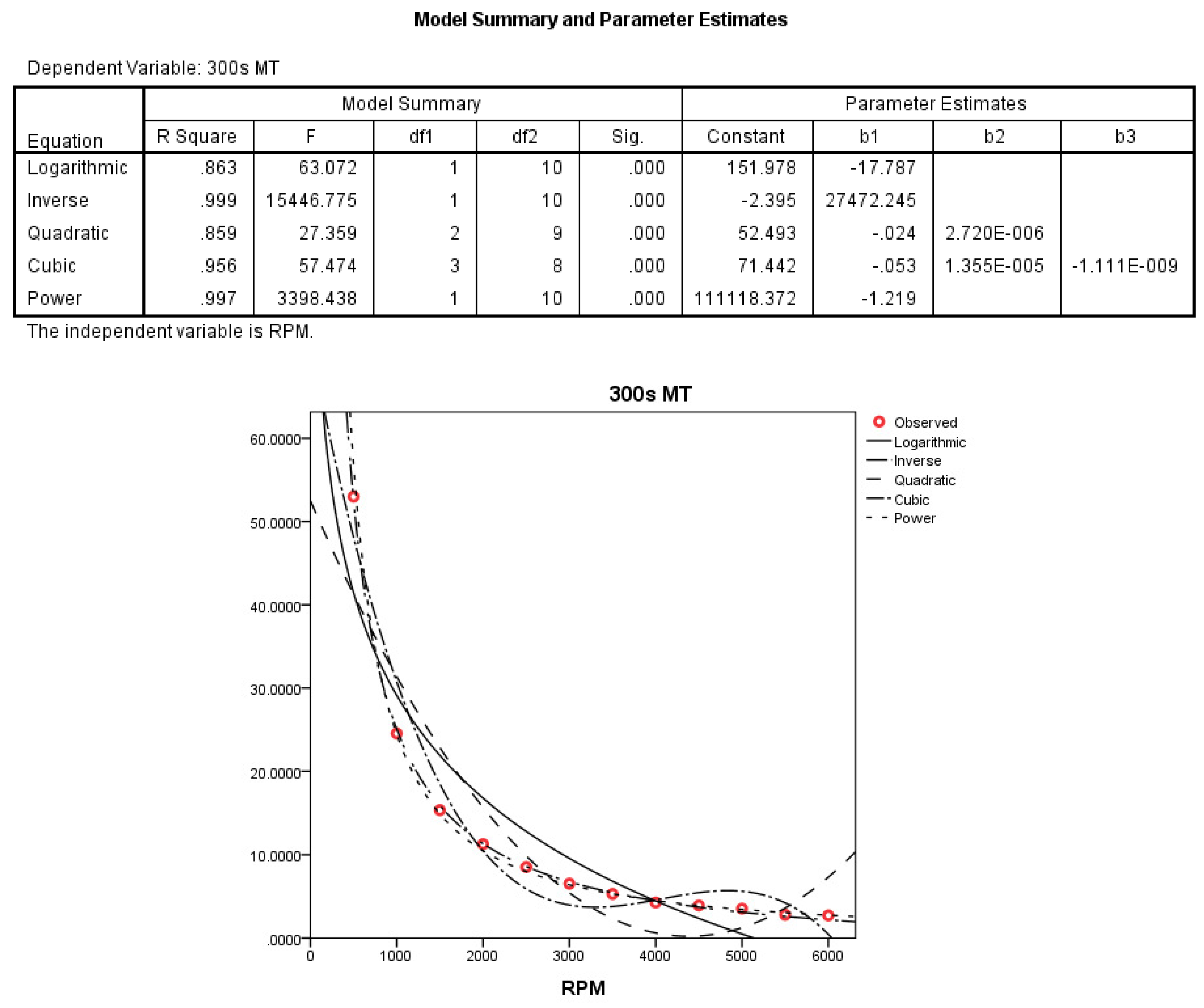
Step 1. We use the Curve Estimation of the regression analysis from the SPSS to make a curve estimate for the MT value of
Table 1 above. There are 11 models available in the curve estimation menu. Among these, we select five models with the possibility of being suitable for MT data. They are Logarithmic, Inverse, Quadratic, Cubic and Power models. The results of the analysis are as follows (
Figure 1).
As shown in
Figure 1 above, we can choose the power model and the inverse model based on the value of the coefficient of determination. The estimated functions are given by the formulas
and
Both estimated functions are suitable for reducing the difference in film thickness mentioned above. It is also possible to select and use what is applicable to each company. Then, we obtain
Table 2 involving the estimated function value and
(coefficient of determination) value with respect to the MT value.
As shown in
Table 2 above, MT value and estimated function value are each somewhat different. To compensate for this, we implement the next step.
Step 2. Let
denote the difference of the TT value and the MT value. That is to say, let
= TT −MT. Then, we obtain
Table 3 below.
We then perform the curve estimate for the
value by using the SPSS. We will use the Logarithmic model and the Inverse model as selected in Step 1. The results of the analysis are as follows (
Figure 2).
Thus, the estimated functions are given by the formulas
and
By using these functions, the estimated functions are given by the formulas
and
All four estimated functions given are suitable for reducing time and cost in the spin-coating process. To reduce the difference further, the following comparisons are made. The data obtained by each functions are given by the following
Table 4 below.
The function that the best describes the measured thickness (MT) value among the functions derived in Steps 1 and 2 undergo several iterations until the smallest error (see
Table 5) is achieved. Here, the sum of squares error (SSE) is given. The red value for each RPM represents the smallest difference.
To test compliance, we decide to use function with the smallest SSE value to approximate MT value. It is
Step 3. We now establish the following hypothesis to test the function
and the consistency of MT value. Let
and
be population means of MT values and the estimated function
, respectively. Then, we formulate the following research hypothesis.
To test this hypothesis, the results of the paired Samples
t-test at a significant level
are as follows (
Figure 3).
Therefore, we accept the null hypothesis (
) to obtain the statistical basis for estimating
as an approximation of the MT value. From Steps 1 through 3, the best-estimated function corresponds to a fixed time of 300 s; i.e., the function given by Equation (
8) is the best curve estimate for a fixed time of 300 s.
2.2. Fixed RPM at 1000
By the similar method as in
Section 2.1, we can obtain the estimated function of the following case of fixed RPM at 1000. Then, the estimated function is given by the formula
We also can compare the TT value, the MT value and the estimated function value as the following
Table 6.
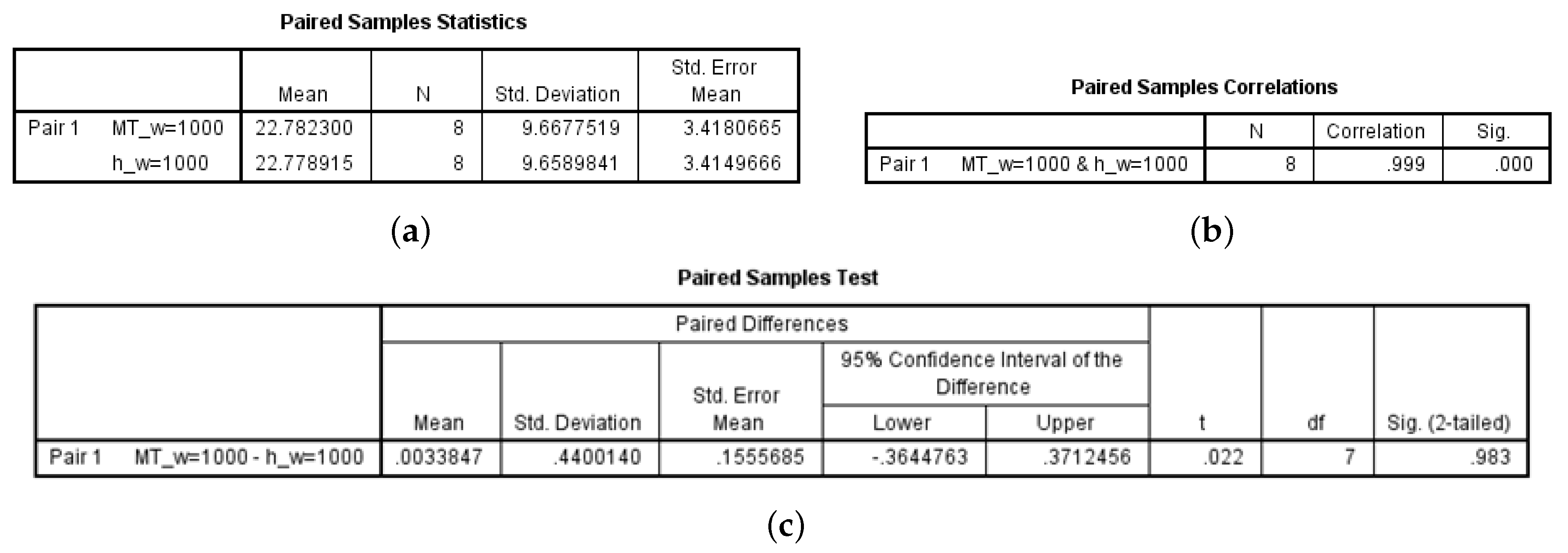
The statistical hypothesis test of the estimated function
is as follows. The results of the paired Sample
t-test to verify the homogeneity of the two groups, as shown in Step 3 of
Section 2.1, are as follows (
Figure 4).
Therefore, we have a statistical basis to conclude that populations in both sample spaces are equal to each other at a significant level .
2.3. Other Cases
Through the process same as in cases
and
above, we obtain estimated functions for the time fixed at 450 and 600 s and the RPM fixed at 2000 and 3000. First, when the time is fixed at 450 and 600, we obtain estimated functions by setting the RPM as a variable as follows:
and
Table 7 is about the value of MT
and MT
, and estimated function values.
Results of the
t-test for estimated function values and MT values are as follows (in
Figure 5), respectively.
Therefore, we see that the mean of populations of estimated functions and MT values are the same at a significant level .
Next, when the RPM is fixed, we obtain estimated functions for the time parameter
and
We get MT
, MT
and estimated values as shown in
Table 8.
The results of the
t-test are as follows (in
Figure 6):
In addition, we see that the mean of populations of estimated functions and MT values are the same at a significant level .
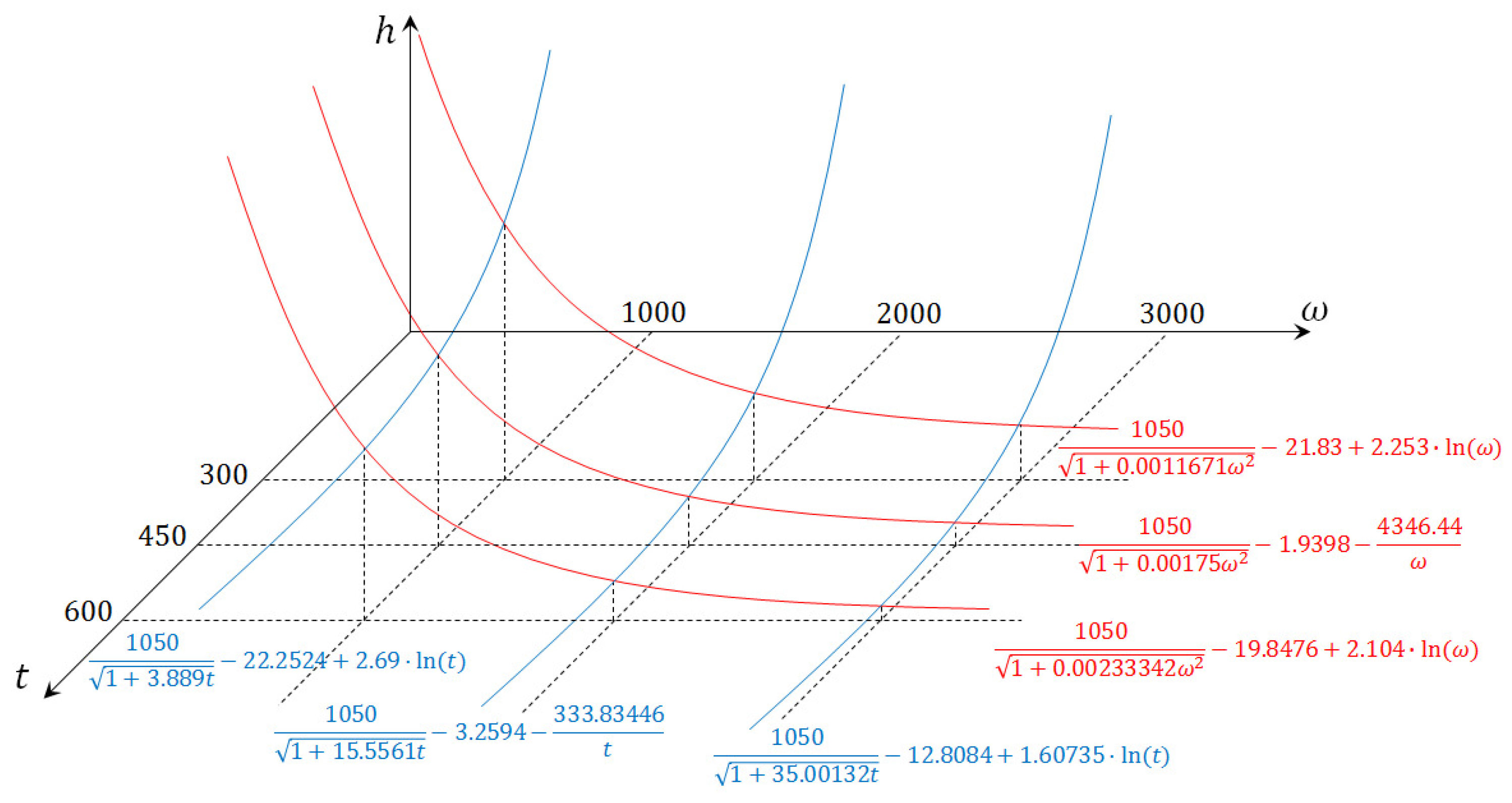
From
Section 2.1,
Section 2.2 and
Section 2.3, we derived a curve-estimated function for each case.
Figure 7 shows that all functions provided an estimate that was statistically equivalent to the MT values. These results suggest that the estimated function can be induced for other RPMs and times.
4. Application: Target Verification
In this section, we try the target verification. We first set the target thickness and thus obtain the required time or RPM for each cases. Finally, we again conduct an experiment. The maximum rotation time for the Spin Coater ACE-200 is 999 s. Thus, the likelihood of error in the coating thickness estimations below and above is high.
The following table shows the results obtained by using the curve estimation function obtained in
Section 2 when the RPM is fixed at
and 3000, and the rotation time
t is fixed at
and 600, respectively (see
Table 12).
With regard to
Table 12, we discuss the thickness value for the parameters specified. When the RPM is fixed, there is no value at
, as shown in the table. Because the function
has a local minimum value
at
, there is no value from
to
. Therefore, when a thickness of
to
is desired, a speed higher than 1000 RPM is required. Additionally, because the ACE-200 system has a maximum spin time of 999 s, it cannot provide a thickness in the desired range of
to
when
. We give the following summary in
Table 13:
In another experiment, the rotation time
t is held fixed at
and 600 s. To obtain the desired thickness, as shown in
Table 12, the RPM could be adjusted for the fixed time frame. In contrast to the previous case in which the RPM was fixed, here we are able to adjust the RPM to produce the desired thickness within the allowable range, given a fixed rotation time. Therefore, it appears to be more effective to fix the rotation time
t to obtain the target film thickness in spin coating processes.
Table 14 lists the thicknesses determined by substituting RPM for the rotation time
t for each coating thickness into
from
Section 3. To compare these values with MT values, we prepare three samples in which the rotation time is fixed at 450 s. The MT
values in the following table represent the average values of the raw data of the three samples.
Actually, this result indicates that the results in
Section 2 and
Section 3 and the values observed by the experiment are the same within the margin of error.
5. Conclusions
5.1. Importance of Results and Formulas in This Paper
Spin coating technology is useful in modern industrial society. However, it still relies on Formula (7), which was introduced in the 1950s, to determine spin coating film thickness. This conventional approach requires extensive time and experimentation to obtain the desired coating thickness, which increases costs. Here, we propose an alternative to this conventional approach. Using the function
, we can estimate the desired coating thickness given the rotation time and RPM, according to the conditions of the coating device. The coating thicknesses achieved using the proposed approach were within the error range expected. In an example described in
Section 4, we were able to obtain the coating thickness based on a fixed rotation time and RPM, using the six functions developed in
Section 2. Additionally, the binary function
estimated in
Section 3 allows users to simulate the desired thickness without having to perform an actual experiment. As a result, many spin coating companies will save time and money using the method implemented in this study.
5.2. Another Approach
Our original goal was to express the equation for thickness of the film fabricated by spin coating as a new binary function. In
Section 2, curved estimates were determined for each fixed variable, and, in
Section 3.1, an approximation of the polyhedron function was acquired through the plane approximation method. In the next research work, we will attempt to obtain an approximation of the equation for thickness of the film fabricated by spin coating as a binary function of the curved estimate and polyhedron function. In
Section 3, we split the domain
D using points
through
. Using a similar method, we obtained the function
with
n-splitting points. Then,
. By adding more splitting points, we can derive the function
as the limit of
. That is,
5.3. Expected Results
In this study, we estimated the bivariate function by assuming rotation time and RPM as independent variables, while the other factors remained fixed. However, the factors affecting the actual coating thickness are , , and . Thus, the addition of other variables to the function formula should improve the accuracy of the spin coating thickness prediction. Considering all of the factors that affect thickness would make the formula too complex, but given that spin coating companies use fixed coating materials, and can be considered constants.
Therefore, in future studies, we will attempt to estimate a three-variable function by setting the independent variables t, , and .
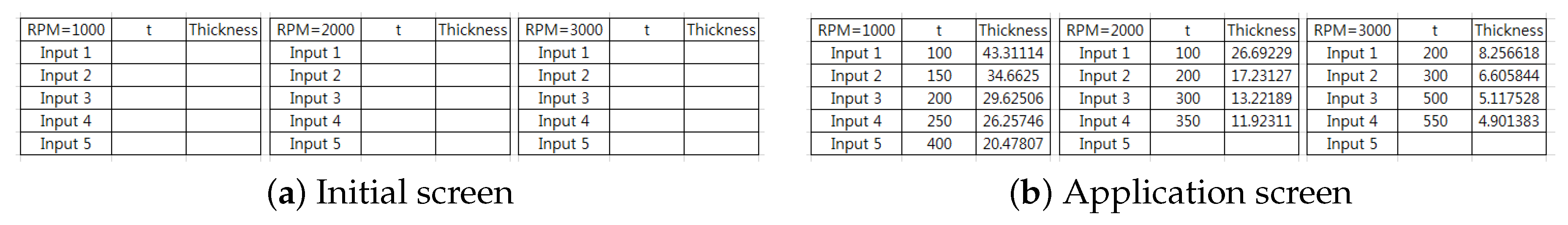
5.4. Capture of the Thickness Calculator by the Excel Program
Based on the results of this study, we developed a thickness calculator using the Microsoft Office Excel program (Microsoft Corp., Redmond, WA, USA). Here, we show screen shots of the initial screen and application screen of the calculator. This calculator can predict the thickness without actual experimentation. As you can see in
Figure 12,
Figure 13 and
Figure 14 below, they are shown for
and
. We will supply our calculator to companies free of charge, in order to help them achieve the desired coating thickness in spin coating processes.
We finish this paper by giving a remark.
Remark 2. We are working on data at fixed conditions of 300 s, as well as different times or fixed RPM conditions, and we will do further research. As shown in Figure 15 below, the experiment was conducted under different conditions, and it was confirmed that the thickness was changed due to the parameters that were not considered in the existing equation. For example, when the aging time is given after spin coating for a fixed condition of 300 s, the thickness changes as shown in the attached figure and the equation, and the equation obtained through curve estimation also changes. In addition, it is expected that process conditions for the manufacture of the desired thickness can be derived simply. In addition, it will be possible to apply to other materials, and further experiments are planned.


