Abnormal Water Quality Monitoring Based on Visual Sensing of Three-Dimensional Motion Behavior of Fish

Abstract

In the context of the problem of water pollution, the movement characteristics and patterns of fish under normal water quality and abnormal water quality are clearly different. This paper proposes a biological water quality monitoring method combining three-dimensional motion trajectory synthesis and integrated learning. The videos of the fish movement are captured by two cameras, and the Kuhn-Munkres (KM) algorithm is used to match the target points of the fish body. The Kalman filter is used to update the current state and find the optimal tracking position as the tracking result. The Kernelized Correlation Filters (KCF) algorithm compensates the targets that are lost in the tracking process and collision or occlusion in the movement process, reducing the errors caused by illumination, occlusion and water surface fluctuation effectively. This algorithm can directly obtain the target motion trajectory, avoiding the re-extraction from the centroid point in the image sequence, which greatly improves the efficiency. In order to avoid the one-sidedness of the two-dimensional trajectory, the experiment combines the pixel coordinates of different perspectives into three-dimensional trajectory pixel coordinates, so as to provide a more authentic fish swimming trajectory. We then select a representative positive and negative sample data set; the number of data sets should have symmetry. The base classifier capable of identifying different water quality is obtained by training. Finally, support vector machine(SVM), eXtreme Gradient Boosting (XGBoost) and pointnet based classifiers are combined into strong classifiers through integrated learning. The experimental results show that the integrated learning model can reflect the water quality effectively and accurately under the three-dimensional trajectory pixel coordinates of fish, and the recognition rate of water quality is above 95%.

1. Introduction

Water is an important resource for human survival. The water resource problem has become a global problem. The water resources that can be exploited and utilized by human beings are decreasing rapidly. With the continuous development of industry and urban construction, industrial and domestic sewage is increasing. Water quality pollution monitoring is of great significance in the field of water environment safety protection. At present, most experts carry out pollution analysis based on the comprehensive pollution evaluation index of water quality collected by physical and chemical analysis technology and automatic detection technology, thus obtaining the pollution status [1]. However, this method cannot carry out long-term and systematic monitoring of water quality. Generally, monitoring is instantaneous and requires a lot of manpower, material resources and financial resources. The actual situation of water quality cannot be effectively reflected through monitoring results, which seriously affects the management and management of water environment.

In response to the above questions, biological monitoring technology has attracted people’s attention in water quality monitoring due to its advantages of real-time, comprehensive, enrichment, continuity, high response sensitivity and intuitiveness. In bio-monitoring technology, most scholars determine fish behavior in a particular water quality environment, obtain sports behavior parameters through vision, and study water quality safety evaluation model based on parameters. Cigdem Beyan et al. [2] present a rule-based trajectory filtering mechanism to extract normal fish trajectories which potentially helps to increase the accuracy of the abnormal fish behavior detection systems. Rui Nian et al. [3] apply a simple yet effective, real-time and robust of fast compressive tracking algorithm with an appearance model to focus on the motion trajectories of underwater fish. Kim [4] Zheng [5], Heng [6], Chen [7] and others use the swimming speed, rotation angle, respiratory frequency changes of fish and curvature and proximity features based on the two-dimensional motion trajectory of fish as factors for water quality evaluation, which reflect the water environment quality from multiple angles comprehensively to some extent. However, there are problems with these studies: first, the amount of tracking calculation for multiple fish is large, the real-time performance is poor, and the accuracy is low. Second, the above studies are all aimed at the trajectory movement of fish in the two-dimensional plane. In fact, fish swim in a three-dimensional space. So the two-dimensional characteristic parameters cannot describe the actual motion state of fish accurately. The processing of three-dimensional images has deeper computational features. Zhang Congxuan [8] et al. proposed a method of 3D motion estimation and depth reconstruction based on image pyramid optical flow to solve the problem of 3D motion estimation and depth reconstruction based on the image sequence optical flow; Adam Michael Stewart [9] et al. used the three-dimensional trajectory of adult zebrafish to simulate the activities of human brain surface in order to understand the pathophysiology of neuropsychiatric disorders better.

There are some problems that cause great interference with using computer vision to monitor water quality. These include the dynamic and multi-objective environment of water, and when the two-dimensional trajectory pixel coordinates reconstitute the pixel coordinates of the three-dimensional trajectory, the error occurs due to the difference between the refractive index of water and the refractive index of air. Therefore, in this paper the predicted value obtained by the Kalman Filter [10] mathematical model and the measured value obtained by the mobilenet [11] -ssd [12] target detection model are matched by the kuhn-munkres [13] (KM) algorithm, and then use the Kalman filter to obtain the predicted values and measured values for data, update the current state, and find the optimal tracking location as the tracking result. Due to the instability in the tracking process, this paper uses the Kernelized Correlation Filters (KCF) [14] tracking algorithm to compensate for the moving target of the fish with collision or occlusion during the motion process. The final result of the above process will extract the pixel coordinate points of the two-dimensional trajectory, and calibrate the two-dimensional pixel coordinate points through direct linear transformation (DLT), to determine the corresponding points of the image, then use the corresponding points as matching points to calculate the three-dimensional pixel coordinates of the fish motion trajectory. In terms of model selection, we use pointnet [15], support vector machine (SVM) [16], eXtreme Gradient Boosting(XGBoost) [17] as base classifiers to integrate to strong classifiers. The input of pointnet is a three-dimensional motion trajectory image, and the input of SVM and XGBoost are feature parameters extracted from three-dimensional trajectory coordinate points, which are integrated by the Multiclass Alpha Integration of Scores (MAIS) [18] method. The semantic mapping model of fish motion behavior characteristic parameters and water quality environment is established to finally realize the judgment of normal water quality and abnormal water quality. The specific process is shown in Figure 1.

2. Fish Target Tracking

2.1. Fish Body Detection

Before tracking fish, first find the location of the fish. We used the MobileNet_SSD detection model under the caffe [19] framework to detect fish and indicate the location of the fish. MobileNet is a lightweight deep network model. It uses a Depthwise Separable Convolution [20] to decompose the standard convolution kernel. Two hyperparameters, width multiplier and resolution multiplier, are introduced to reduce the size of the input and output channels and input and output feature maps, which speeds up the detection. MobileNet_SSD adds 8 convolution layers behind the conv13 of Mobilenet, and then extracts a total of 6 layers for detection, improving detection accuracy. Here, we compare the three network architectures of Faster R-cnn [21], You only look once (YOLO) [22] and Mobilenet_ssd. In the course of the experiment, because this paper mainly studies the analysis of fish behavior, the above three network frameworks are used to compare the detection accuracy. We mainly judge the recall, the precision and the number of FPS (Frames Per Second). The abnormal water quality judgment can be understood as a two-category problem. There are two categories in the sample. There are four combinations of the model prediction result and the real label: TP (actually positive sample, predicted as positive sample), FP(actually negative sample, predicted as positive sample), FN (actually positive sample, predicted as negative sample), TN (actually negative sample, predicted as negative sample). Recall is the proportion that is positively predicted to be positive in all cases. Precision is the proportion of positive predictions that are positive for all predictions. The specific formula is as follows:

$$Recall=\frac{TP}{TP+FN}$$

(1)

$$Precision=\frac{TP}{TP+FN}$$

(2)

As shown in the

Table 1. Performance comparison of network structure in tracking fish.

Model	Recall	Precision	FPS
Faster R-cnn	48.3	75.4	7
YOLO	30.1	66.5	40
Mobilenet_ssd	45.5	72.3	30

:

As can be seen from Table 1, although Faster R-cnn exceeds Yolo and Mobilenet_ssd in accuracy, it sacrifices speed because it exceeds the recommended area. For tracking, it is difficult to achieve high-precision tracking if it is slow. If we only pursue speed, we can prefer to use YOLO. It can be seen that this algorithm is superior in speed to the other two algorithms, but sacrifices the accuracy of detection. The Mobilenet_ssd selected in this paper is somewhere in between. The algorithm is faster than Faster R-cnn and more accurate than YOLO, so it is the best choice for tracking fish movement behavior.

2.2. Fish Tracking

Compared with the detection of other objects, fish have fast swimming speed and small differences between individuals, so it is easy to lose detection targets. In the tracking process, changes in illumination, fluctuation of water surface and shaking of camera will all cause large detection errors. Solving the robustness, accuracy and rapidity in the tracking process is very important for water quality monitoring by using fish movements. The traditional target detection algorithm uses the sliding window method to judge all possible regions in turn. Although this method can realize the Partial area target detection, the image pixel features will be extracted repeatedly, which is extremely slow and cannot achieve a real-time effect in subsequent tracking. As shown in Figure 2, this paper first uses Mobilenet_ssd to detect the target fish in the water, and frame the target fish through a rectangular frame to find the central coordinate point (x, y). There are a total of 7 red mullet in the trial. When we capture the first frame, we need to create a Tracks and assign trackID for each red mullet. The KM algorithm is used to perform feature point matching, and the Intersection over Union (IOU) between the predicted position of the current frame and the current frame target detection frame is calculated. After many experiments, we set the IOU threshold to 0.4. If the calculated IOU is less than 0.4, it determines that the current match is invalid, and then uses the KM algorithm to re-determine and assign the trackID. If the IOU is greater than 0.4, the current match is maintained. Then, the boundary frame obtained by the Kalman filter prediction and the bounding box obtained by the target detection algorithm are used to update the current state, but the frequent trackID switching also loses some targets, resulting in inaccurate tracking count. Therefore, the KCF tracking algorithm is used here to compensate for the fish moving target that is lost or occluded during the motion and the occlusion, and the optimal tracking result is obtained. Figure 2 is a tracking process diagram.

2.2.1. Kalman Filter Algorithm

The Kalman filter uses mathematical modeling to obtain the target fish’s predicted value and the detected observation value for data fusion to find the optimal estimated value. When we want to know the exact bbox of one of the target fish at t frame time, it is recorded as $bbo{x}_0$. The bbox of the target in the 1 to $t-1$ frame is known. Now we have two ways to get the bbox of the t frame: First, through mathematical modeling, the bbox of the t frame is predicted based on the information of 1 to $t-1$, which is recorded as $bbo{x}_p$. The second is to directly measure the bbox of the t frame by the target detection algorithm, which is recorded as $bbo{x}_m$. What Kalman filter does is use $bbo{x}_p$ and $bbo{x}_m$ to get $bbo{x}_0$. It is implemented in two steps: predict, that is calculated $bbo{x}_p$ by mathematical model; update, combine the measured values $bbo{x}_m$ to get the best estimate $bbo{x}_0$ of the current state.

We predict state vector u and variance of uncertainty P (covariance)

$${u^{{}^{\prime }}}_{k|k-1}=F{u^{{}^{\prime }}}_{k-1|k-1}$$

(3)

$$P_{k|k-1}=F{P}_{k-1|k-1}{F}^T+Q$$

(4)

where, u: previous state vector; P: previous covariance matrix; F: state transition matrix (captures state transition from one time step to another); Q: process noise matrix.

We correct or update state vector u and variance of uncertainty P (covariance).

$$C=A{P}_{k|k-1}{A}^T+R$$

(5)

$$K_k=P_{k|k-1}{A}^T{C}^{-1}$$

(6)

$${u^{{}^{\prime }}}_{K|k}={u^{{}^{\prime }}}_{k|k-1}+K_k(b_k-A{u^{{}^{\prime }}}_{k|k-1})$$

(7)

$$P_{k|k}=P_{k|k-1}-K_{k}C{K}^T$$

(8)

where, u: predicted state vector; A: matrix in observation equations; b: vector of observations; P: predicted covariance matrix; Q: process noise matrix (or covariance matrix of system error); K: Kalman Gain matrix (based on recursive least squares); C: covariance weighting matrix (with variance along diagonal); R: observation noise matrix.

Kalman filtering is used to estimate the state of the fish tracking system in two ways: a priori estimate and a posteriori estimate. The prior estimate refers to the estimation of the state before the observation is obtained, and the a posteriori estimate is further corrected based on the prior knowledge after obtaining the observation. Therefore, in the process of dealing with the actual tracking problem, the initial state of the Kalman filter is difficult to determine accurately. It is necessary to give an approximate value according to the prior knowledge, and continuously adjust the parameters and correct it according to the posterior knowledge. The initial state of u is roughly estimated based on the camera pose, the swimming speed of the fish, and the direction of the fish head. F is the state transition matrix, which is a conjecture model for the transformation of the target state. The state transition matrix is used to model the moving target. For fish, it may be uniform motion or uniform acceleration motion. We assume that the fish are moving at a uniform speed under normal water quality, and the fish are uniformly accelerated under abnormal water quality. In the Kalman filter tracking system, P is the predicted covariance matrix, which indicates our trust in the current prediction state. The smaller it is, the more we believe the current prediction state. Its value determines the initial convergence speed, generally starting with a smaller value in order to obtain a faster convergence speed. With the iteration of the Kalman filter, the value of P will change continuously. When the tracking system enters the steady state, the p value will converge to a minimum estimated variance matrix. The Q value is process noise. The smaller the tracking system is, the easier it is to converge. The higher the value of the model predicts the value, but the smaller the value, the easier it is to diverge. If Q is zero, then we only believe the predicted value. The larger the Q value, the lower the trust we have for the prediction, and the higher the confidence in the measured value; if the Q value is infinite, then we only trust the measured value. R value is the measurement noise, too small too mostly is not appropriate. If R is too large, the Kalman filter response will be slower because it reduces the trust in the newly measured values. The smaller the R, the faster the system converges, but when it is too small, it is prone to shocks. Therefore, in the process of debugging parameters, first adjust Q from small to large, and adjust R from large to small. First fix a value to adjust another value to see the convergence speed and waveform output.

2.2.2. KM Algorithm

The KM algorithm is a data matching algorithm. What we need to solve the tracking target is the feature point matching problem between $t-1$ frame and t frame. All feature points between the phase difference frames can form two sets X and Y, there are m feature elements in the set set X, and n feature elements in the set Y. The function of the KM algorithm is to match the feature elements in X and the feature elements in Y by weights. What we have to do in this experiment is to match the bbox of the $t-1$ frame target fish and the bbox of the t frame target fish by weights to complete the tracking.

2.2.3. Correlation Filtering

The KCF divides the target area and the background area of the current frame into positive samples and negative samples, and uses the machine learning method to train the positive and negative samples to obtain the classification model. In the next frame, the trained classification model is used to find the optimal region for tracking. In the experiment, if the continuous multi-frame does not achieve the IOU matching of the predicted target fish predicted position and the detection frame position, the target fish is considered to disappear. Disappearing target fish is tracked and compensated by KCF, thus avoiding the problem of tracking loss, incorrect counting, and improving tracking efficiency.

2.2.4. IOU Calculation

According to the experimental results, it can be concluded that the use of IOU can solve the error caused by the occlusion between the illumination and the target during the target tracking process.When the target is occluded or exposed to light, an obstruction is detected or nothing is detected. That is, the original target is not detected, and it is assumed that the occlusion is associated with the original target.Then, after the occlusion or illumination ends, because the target IOUs of similar size tend to be large, the correct association can be quickly restored. Figure 3 shows the relationship between the predicted border and the detected border in the IOU:

It can be seen that the IOU calculates the ratio of the intersection and the union of the “predicted border” and the “detected border” which is:

$$IOU=\frac{\mathrm{PredictionResult}\cap \mathrm{DetectionResult}}{\mathrm{PredictionResult}\cup \mathrm{DetectionResult}}=\frac{area}{area1+area2-area}$$

(9)

Among them, the width of area1 is: $W_1=X_{12}-X_{11}$; High is: $H_1=Y_{12}-Y_{11}$; the width of area2 is: $W_2=X_{22}-X_{21}$; high is: $H_2=Y_{22}-Y_{21}$; the width of the area is: $W=W_2+W_1-(X_{22}-X_{11})$; high is: $H=H_2+H_1-(Y_{22}-Y_{11})$.

When IOU = 0, which is $X_{12}<X_{21}$ or $Y_{12}<Y_{21}$, there is no public area for the predicted border and the detection border.When IOU < 0.4, the match fails. When IOU > 0.4, the current match is maintained and the state is updated using Kalman filtering. Figure 4 shows the tracking effect.

Figure 5 is a flow chart showing the effect of continuously updating the tracking state by Kalman filter and tracking compensation of the target fish by using correlation filtering during the target fish tracking process. Figure 5a shows the effect of assigning each fish to a trackID. Figure 5b shows when one of the fish is continuously tracked in a continuous image of a sequence and its position in the subsequent image is tracked, feature tracking is used to achieve a smoothing effect of the trajectory.

3. 3D Trajectory Pixel Coordinate Reconstruction

In the experimental test, the fish will tend to swim along the cylinder wall. If a single camera is used to collect video images, the swimming information of the fish is one-sided and some features parameters will be ignored whether the camera is placed in front or above. Therefore, in order to obtain more parameter features and improve the accuracy of water quality anomaly judgment, it is a key step to obtain the basic data of fish spatial trajectory. Therefore, the experiment will have two-dimensional images captured by two cameras, which will be transformed into the relationship between the research objects in the three-dimensional space. During the shooting process, it must be ensured that both cameras are activated at the same time with no time delay. During the conversion process, due to the difference between the light refractive index of water and that of air, errors in three-dimensional reconstruction may occur. In order to reduce this error, calibration must be used. In the experiment, direct linear transformation (DLT) [23] was used to calculate the desired calibration coordinates by combining the realistic coordinates with DLT parameters, and the average error was reduced by comparing with the measured realistic world coordinates.

In the experiment, the basic problem to be solved is to find out the mathematical relationship between the coordinates of the three-dimensional point and its projection onto the image plane. The specific algorithm flow is shown in Algorithm 1.

Algorithm 1 Camera calibration and point reconstruction based on direct linear transformation (DLT)

1:Camera calibration by DLT using known object points and their image points.

This code performs 2D or 3D DLT camera calibration with any number of views (cameras).

Iuput

nd is the number of dimensions of the object space: 3 for 3D DLT and 2 for 2D DLT.

xyz are the coordinates in the object 3D or 2D space of the calibration points.

uv are the coordinates in the image 2D space of these calibration points.

The coordinates (x,y,z and u,v) are given as columns and the different points as rows.

For the 2D DLT (object planar space), only the first 2 columns (x and y) are used.

There must be at least 6 calibration points for the 3D DLT and 4 for the 2D DLT.

Ouput

L:array of the 8 or 11 parameters of the calibration matrix

err:error of the DLT (mean residual of the DLT transformation in units of camera coordinates).

2:Reconstruction of object point from image point(s) based on the DLT parameters.

This code performs 2D or 3D DLT point reconstruction with any number of views (cameras).

For 3D DLT, at least two views (cameras) are necessary.

Input

nd is the number of dimensions of the object space: 3 for 3D DLT and 2 for 2D DLT.

nc is the number of cameras (views) used.

Ls (array type) are the camera calibration parameters of each camera (is the output of DLT

calib function). The Ls parameters are given as columns and the Ls for different cameras as

rows.

vs are the coordinates of the point in the image 2D space of each camera.

The coordinates of the point are given as columns and the different views as rows.

Ouput

xyz: point coordinates in space

3:Normalization of coordinates (centroid to the origin and mean distance of sqrt (2 or 3)

Iuput

nd:number of dimensions (2 for 2D; 3 for 3D)

x:the data to be normalized (directions at different columns and points at rows)

Ouput

Tr:the transformation matrix (translation plus scaling)

x:the transformed data

3D Trajectory Synthesis

Compared with the time series of traditional two-dimensional trajectory, the three-dimensional trajectory motion can provide a more real fish swimming trajectory, it can reduce the potential error of the lateral motion of fish facing the camera as much as possible, and converts the three-dimensional data into a visual trajectory, to provides a visual representation method of fish motion for experimental research.

If the stereo matching and tracking are treated as two mutually independent processes, when the number of fish schools increases, the frequency of each fish approaching or blocking each other in the swimming process is very high, resulting in a short slice of extracted two-dimensional trajectory segments, and the uncertainty of stereo matching is difficult to eliminate in a short time using motion features. If the centroid points of the extracted fish are superimposed on one another or move too close to each other when swimming for too long, the trajectory synthesized by the centroid points will be seriously missing, thus will cause errors in 3D reconstruction and affect the reconstruction effect. Therefore, it can be seen that the reconstruction process and the tracking process are interdependent. In this study, three-dimensional point construction and real-time tracking are taken as a whole. In the reconstruction process, two cameras are used to photograph the fish motion at different angles. If the centroid points are close to or overlap at one angle of view, we can jump to another angle of view to eliminate the uncertainty of trajectory tracking. In this way, the centroid coordinates of the fish can be extracted at every time point, and the difficulty of matching the features is greatly reduced.

As shown in Figure 6, the experimental device belongs to monocular multi-view imaging, and the geometric relationship between the two cameras and the fish tank was determined during the design. According to these fixed geometric relations, it is possible to obtain the coordinates of the centroid point positions in which the fish are consistent from two angles of view. According to the experimental device shown in Figure 6, the pixel of the image captured by the front camera are $(X_1,Y_1)$ and the pixel coordinates of the image captured by the above are $(X_2,Y_2)$. Among them, what is described by $X_1$ and $X_2$ is pixel coordinates in the same direction, so the information of X axes of two camera is overlapped. According to DLT, camera distortion is calibrated, and image corresponding points are determined, then the corresponding points are taken as matching points to calculate three-dimensional pixel coordinates of fish motion tracks.

4. Establishment of Classification Model

4.1. The Model Structure of Pointnet

The trajectory of the fish obtained by the experiment consists of a set of points. We extract the features of the point set through the model structure and determine the category to which the trajectory belongs. Pointnet can learn a most favorable network model by learning the pose information of the point set itself. From the data structure, by extracting the two-dimensional motion trajectory of fish, they are combined into a three-dimensional motion trajectory. If the factors such as color, edge, texture, etc., are not considered, only the coordinates of the point are considered, then the motion trajectory is a set of points of $n\times 3$. Then, when the n points are read in different orders, the classification of the images must output the same result. Since the position of the point is fixed in the two-dimensional image, there is no such problem, but in the three-dimensional trajectory data, the input combination of the points has a total of n!, so processing must be performed. Pointnet uses the maximum pooling. After the convolution operation on n points, an $n\times 1024$-dimensional matrix is generated, and 1024-dimensional 1024-global features are obtained. For each dimension, the maximum value is solved, and the problem of disorder is solved.

In the classification problem, the pointnet only needs to process the global features, and the final result can be obtained by performing MLP (Multi-Layer Perception) [24] or SVM classification on the global features. Pointnet combines the extracted global features and point features through the fish trajectory to obtain the feature matrix, and then re-extracts the features of each point based on the feature matrix to obtain the point information including local and global features.

For 3D images, when we target the classification, we should ensure that the results are unchanged when we perform operations such as rotation and upshift. Pointnet performs affine transformation on the original matrix by adding T-net (Transformation networks) [25]. It is equivalent to processing directly in the data preprocessing stage to ensure the invariance of the results. T-net is a subnet of the prediction feature space transformation matrix, which inputs a transformation matrix that is consistent with the feature space dimension. The transformation matrix is then used to multiply the raw data to effect a transformation of the input feature space such that each subsequent point has a relationship with each point in the input data. Therefore, we use the pointnet network model to train the three-dimensional motion trajectory of fish and establish a water quality positive anomaly classifier.

4.2. SVM Water Quality Classifier

Support vector machine is an excellent pattern classifier, which can solve practical problems such as small samples, nonlinear, high dimensional and local minimum. From the perspective of pattern recognition, fish with normal water quality and abnormal water quality have distinctly different motion features, which can be regarded as two different types of exercise patterns. Therefore, abnormal water quality monitoring is a classification problem. For the nonlinear inseparable problem of fish’s motion feature parameters overlap, SVM transforms fish motion feature parameters into linear problems in high-dimensional space by nonlinear transformation, and finds the optimal classification surface in high-dimensional space. Therefore, computer vision and support vector machine can be combined to monitor water quality anomalies.

4.3. XGBoost Water Quality Classifier

XGBoost adds a regular term to the cost function to control the complexity of the model. The regular term reduces the variance of the model, making the trained model simpler and preventing overfitting. This is a generalization of the training of fish motion parameters. Significant improvement in capacity; In the process of collecting data, due to various artificial or experimental defects, data loss will inevitably occur. XGBoost has a built-in rule for handling missing values. The user needs to provide a different value from the other samples and pass it in as a parameter to use as the value of the missing value. XGBoost uses different processing methods when different nodes encounter missing values, and will learn the processing method when missing values are encountered in the future, which provides a good solution for the missing character parameters of fish; XGBoost allows cross-validation to be used in each round of boosting iterations. Therefore, the optimal number of boosting iterations can be conveniently obtained; XGBoost can continue training in the last round of results. This feature is a huge advantage in the application of fish characteristic parameter classification, which can achieve the continuity of the model. So we used XGBoost to replace the previous classifier and build a water quality classification model.

4.4. The Model Merging of SVM and XGBoost Classifiers

Firstly, in the classification process by using SVM and XGBoost, the parameter data about fish behavior and movement characteristic that can reflect the change of water quality are calculated, and the data are processed to make the movement parameter features more prominent. Secondly, all the characteristic parameter samples are integrated to obtain the characteristic parameter set and establish the model for monitoring the abnormality about water quality based on SVM and XGBoost. Finally, to achieve the purpose of monitoring the abnormality about water quality, the model is used to analyze and evaluate the characteristic parameters of fish behavior under the unknown water quality.

Through the experiments, we obtained the three-dimensional motion trajectory of the fish, and further obtained the characteristic parameters of the fish’s motion behavior: velocity, acceleration, curvature, swimming distance of the center, dispersion and so on. The calculation formula is shown in

Table 2. Formula for calculating characteristic parameters.

Features	Formula	Description
Swimming Distance	$d=\sqrt{{(x_1-x_2)}^2+{(y_1-y_2)}^2+{(z_1-z_2)}^2}$	($x_1,y_1,z_1$) and ($x_2,y_2,z_2$) are used to indicate the coordinates of the start and end points on the fish target tracking trajectory per unit time d is the distance the fish swims in t time
Speed	$v=\frac{d}{t}$	d is the distance the fish swims in t time
Acceleration	$a=\frac{v_2-v_1}{\Delta t}$	$v_1$ and $v_2$ represent the speeds of $t_1$ and $t_2$, respectively $\Delta t=t_2-t_1$
Curvature	$k=\frac{A(1+E^2)+B(1+D^2)-CDE}{{(1+D^2+E^2)}^{\frac{3}{2}}}$	$A=\frac{1}{2}\frac{d^{2}z}{d{x}^2}$$B=\frac{d^{2}z}{d{y}^2}$$C=\frac{d^{2}z}{dxdy}$$D=\frac{dz}{dx}$$E=\frac{dz}{dy}$
Dispersion	$L{S}^2=\left\{\begin{array}{c}{\displaystyle \sum _{i=1}^n}{(x_i-\overline{x})}^2\\ {\displaystyle \sum _{i=1}^n}{(y_i-\overline{y})}^2\\ {\displaystyle \sum _{i=1}^n}{(z_i-\overline{z})}^2\end{array}\right.$	The relationship between the overall center of gravity of the fish school $(\overline{x},\overline{y},\overline{z})$ and the position of the center of gravity of each individual $(x_i,y_i,z_i)$

.

4.5. Ensemble Learning

There are different feature extraction methods for images about fish trajectory, and each method focuses on description of image in different aspects. Combined with these features, the feature information can be expressed more comprehensively. We used the traditional monitoring method for water quality based on the support vector machine and XGBoost, and integrated with the present monitoring method named Deep Neural Network. That is, the learning task is completed by constructing and combining multiple learners. The normal and abnormal monitoring method for water quality can be regarded as a dichotomous problem. We use three classifiers (pointnet neural network model, SVM, and XGBoost) to classify on test samples. As shown in

Table 3. Model integration approach.

Combination Strategy	Test Sample 1	Test Sample 2	Test Sample 3
MAIS	$0.012$	$0.015$	$0.008$
Voting method	$0.028$	$0.023$	$0.034$
Average method	$0.021$	$0.022$	$0.027$
Learning method	$0.031$	$0.030$	$0.028$

, in the combination strategy, we used MAIS, voting method, averaging method, and learning method to compare.

MAIS is performed separately on the scores assigned to each class by the classifiers. Thus, the multiclass problem is split into K binary classification problems; The voting method belongs to the minority obeys the majority. The voting method combines the T base classifiers, assuming that the error rates of each base classifier are independent of each other. If more than half of the base classifiers are correct, the integrated classification is correct; The averaging method is a weighting operation on different classifiers. The weights are generally obtained from the training data set. We estimate the error of the individual learner, and then make the weight size inversely proportional to the error size; The learning method first trains the primary learner from the initial data set and then generates a new data set for training the primary learner. Then, using the cross-validation or leave-one method, the training samples of the secondary learner are generated by training the samples that are not used by the primary learner, and iteratively, until the end. It can be seen from Table 3 that the MAIS works best and the output error is minimal. So in the integrated learning method we finally selected MAIS for the final predicted output.

5. Experiment

5.1. The Environment of Experiment

The water for experiment is dechlorinated tap water, which was fully aerated after 24 h. The platform is a circular experimental tank with a diameter of 50 cm and a height of 40 cm to study the movement of red crucian carp under the computer monitoring. The experiment was divided into three groups, each with seven red crucian carp. Using the method of parallel experiments, except for water pollutants being different in the three groups, other conditions are completely consistent. The first group of experiments had two experimental tanks. To one was added a certain volume of experimental water without any pollutants, and the other was added aqueous solution of trichlorfon with concentration of 1.5% in the same volume; The second group also had two experimental tanks. One was added experimental water only, and the other was added oxalic acid solution with a PH value of 3.5 in the same volume; In the third group, one was added experimental water, and the other was added $K_{2}C{r}_2{O}_7$ solution with concentration of 5.75 mg/L in the experimental water. In the process of experiment, charge coupled device(CCD) camera was used to obtain video image of fish movement, and fish video was collected five minutes after the beginning of experiment. The size of each frame is 480 × 640, and the frame rate is 25 frames per second. The experiment adopts the method of parallel experiment. Only pollutants of the water quality are different in the three groups of experiments, and other conditions are completely consistent.

The experimental environment for training and testing is Ubuntu16.04 operating system and depth learning model built on depth learning library. The CPU is Intel’s sixth generation cool I7 6700K, and the GPU is NVIDIA’s flagship graphics card GeForce GTX 1080 released officially.

5.2. Experimental Results and Analysis

Integrated learning is used to build the sample set and extract the characteristic parameters. The specific steps for training and testing the sample set and feature parameters are as follows: (1) The CCD camera is used to collect video frames under normal water quality and abnormal water quality, and 1000 frames of fish trajectory images are selected to extract the feature parameters. (2) The three-dimensional motion trajectory image is sent to pointnet model for training, and the extracted feature parameters are put into SVM and XGBoost for training, then the water quality evaluation base classifier is obtained. (3) Integrate the base classifier to obtain a strong water quality evaluation classifier.

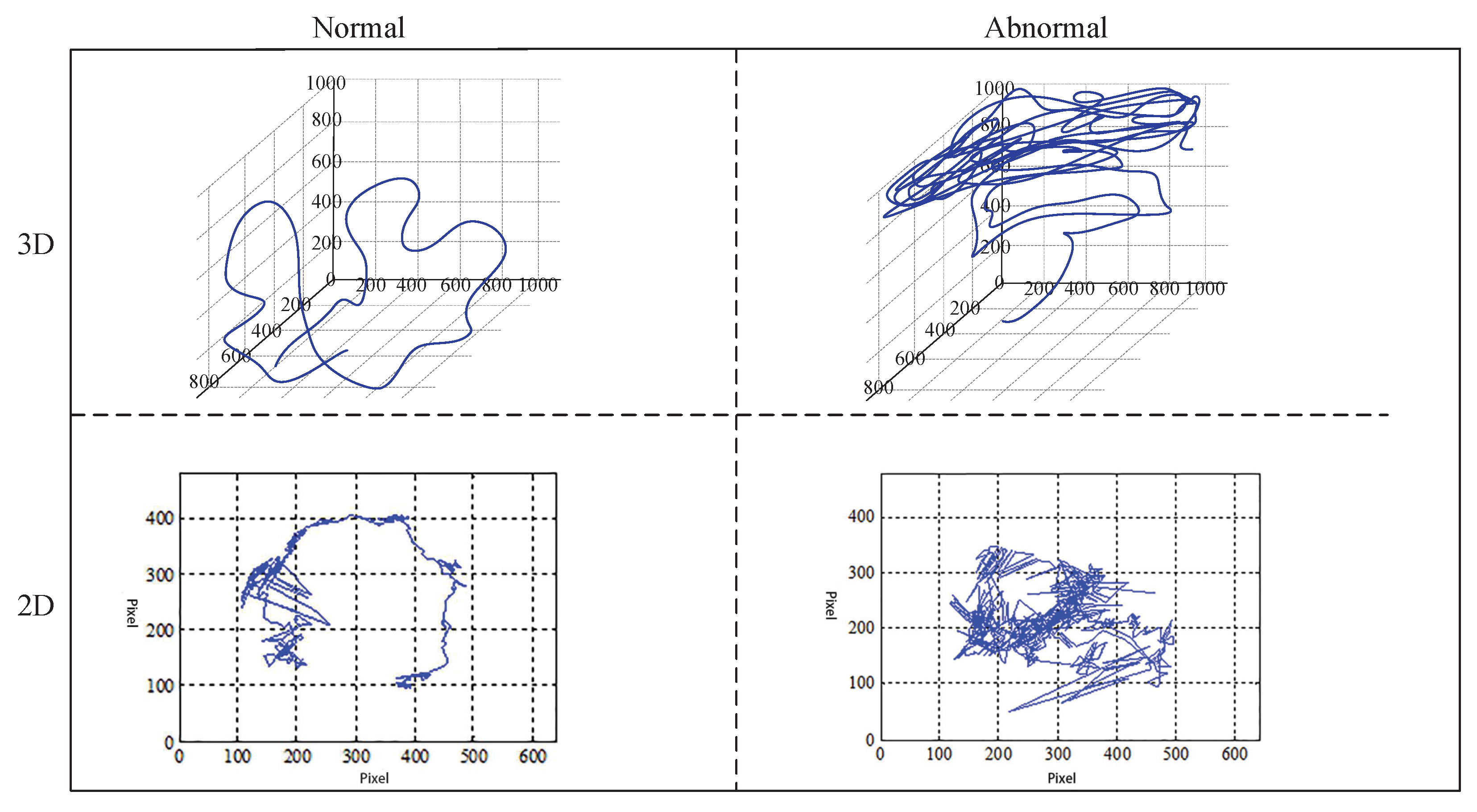
5.2.1. Use Trajectory to Identify Water Quality

Figure 7 shows a comparison figure of fish movement trajectories in different dimensions under normal water quality and abnormal water quality. In the normal water quality, there are fewer pixel points of fish trajectory. That is, the fish move more slowly, and there are fewer swimming states of violent fluctuations and turns, and the trajectory of the fish follows a good arc. However, in the abnormal water environment, there are many pixels of fish trajectory. That is, the fish move faster, and the direction of movement of fish varies greatly. In addition to, the trajectory of the fish does not follow a good arc, and the center of gravity of the fish is close to the center of the fish tank.

5.2.2. The Training and Optimization of Pointnet Model

The sample sets of normal and abnormal water quality were established, and they were input into the model for training to obtain the evaluation model of water quality.

In this experiment, three groups of fish movement trajectory data obtained from experimental water without any pollutants and water added with trichlorfon, oxalic acid solution and potassium dichromate were used for training. As shown in Figure 8, Epoch was set as 100, and with the increase of Epoch, the training accuracy increased gradually.

In the optimization algorithm, we use the stochastic gradient descent (SGD) [26], and one of the key parameters of SGD algorithm is learning rate. As shown in

Table 4. Change of learning rate.

Epoch	Learning Rate
0–65	1 × 10${}^{-3}$
66–85	1 × 10${}^{-4}$
86–99	1 × 10${}^{-5}$

, in the training process, we set different learning rates. The highest accuracy can reach about 95%, that is, the pointnet model selected meets the requirements of water quality evaluation fully.

5.2.3. Extraction of Feature Parameters

As shown in Figure 9, five sets of characteristic parameters including velocity (v), acceleration (a), curvature (k), central swimming distance (d) and dispersion are extracted from the motion trajectory. The blue graph on the left shows the variation trend of characteristic parameters under normal water quality, and the red graph on the right shows the variation trend under abnormal water quality. As can be seen from the figure, the velocity, acceleration and curvature present slight variation under normal water quality, and the average swimming distance d is roughly the same, without drastic fluctuations. The dispersion is relatively small and the situation is stable. Under abnormal water quality, it is obvious that each parameter changes greatly. After the feature parameters are processed, input them in the classification model of SVM and XGBoost for training. Then combined with pointnet to achieve integrated classification, the accuracy is significantly improved.

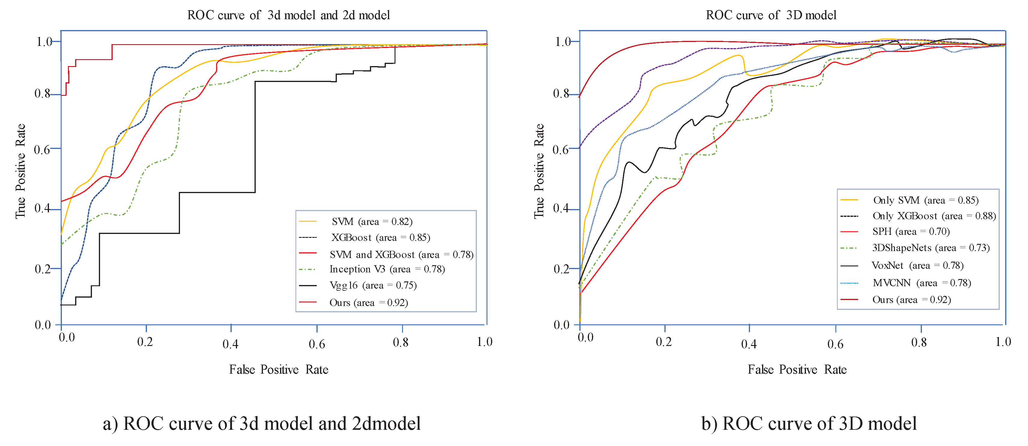
5.2.4. Performance Evaluation

In order to evaluate the performance of the ensemble classifier, we select other 3d classification models for comparison. The results are shown in

Table 5. 3D model performance evaluation.

Model	Input	Accuracy Sample 1	Accuracy Sample 2	Accuracy Sample 3	Accuracy Sample 4
Only SVM	Parameters	87.2	86.5	89.1	90.9
Only XGBoost	Parameters	88.3	91.6	92.3	90.0
SPH [27]	Mesh	65.2	64.3	66.6	69.5
3DShapeNets [28]	Volume	77.8	75.6	77.1	79.6
VoxNet [29]	Volume	80.5	83.4	80.1	82.0
MVCNN [30]	Volume	80.5	83.4	80.1	82.0
Ours	Point	95.5	96.2	95.6	94.9

.

As can be seen from Table 5 that we use the integrated learning method to compare with other methods, and there are clear advantages in terms of accuracy. If use SVM or XGBoost only to classify by feature parameters, the accuracy is not optimal.

Compared the ensemble classifier with the classifier trained by two-dimensional parameters, the results are shown in

Table 6. Performance evaluation of 3d model and 2d model.

Model	Input	Accuracy Sample 5	Accuracy Sample 6	Accuracy Sample 7	Accuracy Sample 8
SVM	Parameters	86.3	82.5	87.9	86.5
XGBoost	Parameters	89.5	90.3	91.1	90.7
Inception v3 [31]	Image	92.3	91.5	90.3	93.8
Vgg16 [32]	Image	90.6	88.1	89.5	90.2
SVM and XGBoost	Parameters	91.9	92.5	92.8	92.5
Ours	Parameters and Point	94.5	95.2	94.6	93.9

.

As can be seen from Table 6, the classifier formed by 2D motion trajectory of fish is not as accurate as 3D. Feature parameters by 2D cannot describe the actual motion state of fish accurately, and 3D image processing has deeper calculation features.

We also selected the Receiver Operating Characteristic (ROC) curve to evaluate the performance of the classifier.The abscissa of the ROC curve is the false positive rate (FPR), which is called the false positive rate, and the ordinate is the true positive rate (TPR), which is called the true positive rate. Its calculation formula is:

$$TPR=\frac{TP}{TP+FN}$$

(10)

$$FPR=\frac{FP}{FP+TN}$$

(11)

In the above formula, P is the number of true positive samples, N is the number of true negative samples, $TP$ is the number of positive samples predicted by the classifier in P positive samples, and $FP$ is predicted by the classifier in N negative samples. The number of positive samples. By calculating the Area under Curve (AUC), which is the area under the ROC curve (Figure 10), the classifier is evaluated. When a positive sample and a negative sample are randomly selected, the current classification algorithm will calculate the Score value based on the value. The probability that this positive sample is in front of the negative sample is the AUC value. The larger the AUC value, the more likely the current classification algorithm is to place the positive sample in front of the negative sample, so that the classifier performance is better.

As can be seen from Figure 10, our method AUC has the largest value and the model performance is significantly better than other algorithms

6. Conclusions

We use two cameras to track the fish body from different angles, and the trajectory is smooth, so as to obtain the position coordinates of the center of mass point consistent with the fish body observed from two perspectives. During the experiment, we combined Kalman filter with KCF to reduce the influence of posture change and illumination change of fish target on tracking stability and realize real-time robust tracking without occlusion. Moreover, in the track visualization, we performed track smoothing while tracking, avoiding the centroid extraction of the image sequence and improving the tracking efficiency. The 3D trajectory movement can provide fish swimming trajectory more real and reduce the potential error in the lateral motion of the fish toward the camera as much as possible, so we use DLT algorithm to determine the corresponding point of the centroid coordinates in the two perspectives and calculate the 3D trajectory coordinates of fish motion. For model training, we use an integrated learning approach that combines a deep model with a traditional machine learning model. Finally, the primary classifier is integrated to obtain the final judgment model of water quality anomaly. Compared to using a single classifier, the integration of the model is better than accuracy and stability. But, due to more training times, the optimal solution has not been reached in time. Water quality monitoring is a real-time process. In the following research, we will further optimize the model, reduce training and test time, enrich the experimental environment, and enhance the robustness of the system. At the same time, we also need to design a more sophisticated grade of water quality to achieve real-time, efficient and stable effect.

References

1. Jang, A.; Zou, Z.; Lee, K.K.; Ahn, C.H.; Bishop, P.L. State-of-the-art lab chip sensors for environmental water monitoring. Meas. Sci. Technol. 2011, 3, 251–259. [Google Scholar] [CrossRef]
2. Beyan, C.; Fisher, R.B. A filtering mechanism for normal fish trajectories. In Proceedings of the 21st International Conference on Pattern Recognition (ICPR2012), Tsukuba, Japan, 11–15 November 2012; pp. 2286–2289. [Google Scholar]
3. Nian, R.; Wang, X.; Che, R.; He, B.; Xu, X.; Li, P.; Lendasse, A. Online fish tracking with portable smart device for ocean observatory network. In Proceedings of the OCEANS 2017, Anchorage, AK, USA, 18–21 September 2017; pp. 1–7. [Google Scholar]
4. Kim, C.M.; Shin, M.W.; Jeong, S.M.; Kang, I.C. Real-time motion generating method for artifical fish. Comput. Sci. Netw. Secur. 2007, 7, 52–61. [Google Scholar]
5. Zheng, H.; Liu, R.; Zhang, R.; Hu, Y. A method for real-time measurement of respiratory rhythms in medaka (Oryzias latipes) using computer vision for water quality monitoring. Ecotoxicol. Environ. Saf. 2014, 100, 76–86. [Google Scholar] [CrossRef] [PubMed]
6. Maa, H.; Tsaib, T.-F.; Liuc, C.-C. Real-time monitoring of water quality using temporal trajectory of live fish. Expert Syst. Appl. 2010, 7, 5158–5171. [Google Scholar] [CrossRef]
7. Chen, J.; Chen, T.; Ma, Z. Application of improved mater-element model in water quality evaluation. Water Resour. Power 2014, 32, 50–52. [Google Scholar]
8. Zhang, C.; Chen, Z.; Li, M. Direct method for 3D motion estimation and depth reconstruction of pyramid optical flow. Chin. J. Sci. Instrum. 2015, 36, 1093–1105. [Google Scholar]
9. Stewart, A.M.; Grieco, F.; Tegelenbosch, R.A.; Kyzar, E.J.; Nguyen, M.; Kaluyeva, A.; Song, C.; Noldus, L.P.J.J.; Kalueff, A.V. A novel 3D method of locomotor analysis in adult zebrafish: Implications for automated detection of CNS drug-evoked phenotypes. J. Neurosci. Methods 2015, 255, 66–74. [Google Scholar] [CrossRef] [PubMed]
10. Welch, G.; Bishop, G. An Introduction to the Kalman Filter; University of North Carolina: Chapel Hill, NC, USA, 1995. [Google Scholar]
11. Howard, A.G.; Zhu, M.; Chen, B.; Kalenichenko, D.; Wang, W.; Wey, T.; Andreetto, M.; Adam, H. Mobilenets: Efficient convolutional neural networks for mobile vision applications. arXiv 2017, arXiv:1704.04861. [Google Scholar]
12. Liu, W.; Anguelov, D.; Erhan, D.; Szegedy, C.; Reed, S.; Fu, C.Y.; Berg, A.C. Ssd: Single shot multibox detector. In Proceedings of the European Conference on Computer Vision, Amsterdam, The Netherlands, 11–14 October 2016; Springer: Cham, Switzerland, 2016; pp. 21–37. [Google Scholar]
13. Zhu, H.; Zhou, M.C.; Alkins, R. Group role assignment via a Kuhn–Munkres algorithm-based solution. IEEE Trans. Syst. Man Cybern. Part Syst. Hum. 2011, 42, 739–750. [Google Scholar] [CrossRef]
14. Henriques, J.F.; Caseiro, R.; Martins, P.; Batista, J. High-speed tracking with kernelized correlation filters. IEEE Trans. Pattern Anal. Mach. Intell. 2015, 37, 583–596. [Google Scholar] [CrossRef] [PubMed]
15. Qi, C.R.; Su, H.; Mo, K.; Guibas, L.J. Pointnet: Deep learning on point sets for 3d classification and segmentation. In Proceedings of the IEEE Conference on Computer Vision and Pattern Recognition, Honolulu, HI, USA, 21–26 July 2017; pp. 652–660. [Google Scholar]
16. Joachims, T. Making Large-Scale SVM Learning Practical. In Advances in Kernel Methods—Support Vector Learning; Schölkopf, B., Burges, C., Smola, A., Eds.; MIT Press: Cambridge, MA, USA, 1999; pp. 169–184. [Google Scholar]
17. Chen, T.; Guestrin, C. Xgboost: A scalable tree boosting system. In Proceedings of the 22nd ACM Sigkdd International Conference on Knowledge Discovery and Data Mining, San Francisco, CA, USA, 13–17 August 2016; pp. 785–794. [Google Scholar]
18. Safont, G.; Salazar, A.; Vergara, L. Multiclass alpha integration of scores from multiple classifiers. Neural Comput. 2019, 31, 806–825. [Google Scholar] [CrossRef] [PubMed]
19. Jia, Y.; Shelhamer, E.; Donahue, J.; Karayev, S.; Long, J.; Girshick, R.; Guadarrama, S.; Darrell, T. Caffe: Convolutional architecture for fast feature embedding. In Proceedings of the 22nd ACM International Conference on Multimedia, Orlando, FL, USA, 3–7 November 2014; pp. 675–678. [Google Scholar]
20. Chollet, F. Xception: Deep learning with depthwise separable convolutions. In Proceedings of the IEEE Conference on Computer Vision and Pattern Recognition, Honolulu, HI, USA, 21–26 July 2017; pp. 1251–1258. [Google Scholar]
21. Ren, S.; He, K.; Girshick, R.; Sun, J. Faster r-cnn: Towards real-time object detection with region proposal networks. In Advances in Neural Information Processing Systems; Curran Associates, Inc.: Red Hook, NY, USA, 2015; pp. 91–99. [Google Scholar]
22. Redmon, J.; Divvala, S.; Girshick, R.; Farhadi, A. You only look once: Unified, real-time object detection. In Proceedings of the IEEE Conference on Computer Vision and Pattern Recognition, Las Vegas, NV, USA, 26 June–1 July 2016; pp. 779–788. [Google Scholar]
23. Abdel-Aziz, Y.I.; Karara, H.M.; Hauck, M. Direct linear transformation from comparator coordinates into object space coordinates in close-range photogrammetry. Photogramm. Eng. Remote. Sens. 2015, 81, 103–107. [Google Scholar] [CrossRef]
24. Longstaff, I.D.; Cross, J.F. A pattern recognition approach to understanding the multi-layer perception. Pattern Recognit. Lett. 1987, 5, 315–319. [Google Scholar] [CrossRef]
25. Li, X.; Bing, L.; Lam, W.; Shi, B. Transformation networks for target-oriented sentiment classification. arXiv 2018, arXiv:1805.01086. [Google Scholar]
26. Robbins, H.; Monro, S. A stochastic approximation method. Ann. Math. Stat. 1951, 22, 400–407. [Google Scholar] [CrossRef]
27. Kazhdan, M.; Funkhouser, T.; Rusinkiewicz, S. Rotation invariant spherical harmonic representation of 3d shape descriptors. In Proceedings of the Symposium on Geometry Processing, Aachen, Germany, 23–25 June 2003; Volume 6, pp. 156–164. [Google Scholar]
28. Wu, Z.; Song, S.; Khosla, A.; Yu, F.; Zhang, L.; Tang, X.; Xiao, J. 3d shapenets: A deep representation for volumetric shapes. In Proceedings of the IEEE Conference on Computer Vision and Pattern Recognition, Boston, MA, USA, 7–12 June 2015; pp. 1912–1920. [Google Scholar]
29. Maturana, D.; Scherer, S. Voxnet: A 3d convolutional neural network for real-time object recognition. In Proceedings of the 2015 IEEE/RSJ International Conference on Intelligent Robots and Systems (IROS), Hamburg, Germany, 28 September–2 October 2015; pp. 922–928. [Google Scholar]
30. Su, H.; Maji, S.; Kalogerakis, E.; Learned-Miller, E. Multi-view convolutional neural networks for 3d shape recognition. In Proceedings of the IEEE International Conference on Computer Vision, Santiago, Chile, 7–13 December 2015; pp. 945–953. [Google Scholar]
31. Szegedy, C.; Vanhoucke, V.; Ioffe, S.; Shlens, J.; Wojna, Z. Rethinking the Inception Architecture for Computer Vision. In Proceedings of the 2016 IEEE Conference on Computer Vision and Pattern Recognition (CVPR), Las Vegas, NV, USA, 27–30 June 2016; pp. 2818–2826. [Google Scholar]
32. Han, S.; Mao, H.; Dally, W.J. Deep compression: Compressing deep neural networks with pruning, trained quantization and huffman coding. arXiv 2015, arXiv:1510.00149. [Google Scholar]
Figure 1. Water quality monitoring flow chart.
Symmetry 11 01179 g001
Figure 2. Track the process.
Symmetry 11 01179 g002
Figure 3. Intersection over Union (IOU) calculation diagram.
Symmetry 11 01179 g003
Figure 4. Tracking effects under normal, lighting, and occlusion.
Symmetry 11 01179 g004
Figure 5. Tracking effect when Kalman filter and Kernelized Correlation Filters (KCF) are combined.
Symmetry 11 01179 g005
Figure 6. Three dimensional trajectory synthesis.
Symmetry 11 01179 g006
Figure 7. Trajectory of fish movement under normal and abnormal water quality.
Symmetry 11 01179 g007
Figure 8. Training accuracy of different pollutants.
Symmetry 11 01179 g008
Figure 9. Feature parameter extraction.
Symmetry 11 01179 g009
Figure 10. Performance evaluation using Receiver Operating Characteristic (ROC) curves.
Symmetry 11 01179 g010