Prototiles and Tilings from Voronoi and Delone Cells of the Root Lattice A_n

Abstract

The orthogonal projections of the Voronoi and Delone cells of root lattice $A_n$ onto the Coxeter plane display various rhombic and triangular prototiles including thick and thin rhombi of Penrose, Amman–Beenker tiles, Robinson triangles, and Danzer triangles to name a few. We point out that the symmetries representing the dihedral subgroup of order $2h$ involving the Coxeter element of order $h=n+1$ of the Coxeter–Weyl group $a_n$ play a crucial role for $h$-fold symmetric tilings of the Coxeter plane. After setting the general scheme we give samples of patches with 4-, 5-, 6-, 7-, 8-, and 12-fold symmetries. The face centered cubic (f.c.c.) lattice described by the root lattice $A_3$, whose Wigner–Seitz cell is the rhombic dodecahedron projects, as expected, onto a square lattice with an $h=4$-fold symmetry.

1. Introduction

Discovery of a fivefold symmetric material [1] has led to growing interest in quasicrystallography. For a review, see for instance [2,3,4]. Aperiodic tilings of the plane with dihedral point symmetries or icosahedral symmetry in three dimensions have been the central research area of mathematicians and mathematical physicists to explain the quasicrystallography. For an excellent review, see for instance [5,6].There have been three major approaches for aperiodic tilings. The first class, perhaps, is the intuitive approach, like Penrose tilings [7,8], which also exhibits the inflation–deflation technique developed later. The second approach is the projection technique of higher dimensional lattices onto lower dimensions, pioneered by de Bruijn [9] by projecting the five-dimensional cubic lattice onto a plane orthogonal to one of the space diagonals of the cube. The cut and project technique works as follows. The lattice is partitioned into two complementing subspaces called $E_{\parallel }$ and $E_{\perp }$. Imagine a cylinder based on the component of the Voronoi cell in the subspace $E_{\perp }.$ Project the lattice points lying in the cylinder into the space $E_{\parallel }.$ Several authors [10,11,12] have studied similar techniques. In particular, Baake et al. [11] exemplified the projection of the $A_4$ lattice. The group theoretical treatments of the projection of n-dimensional cubic lattices have been worked out by the references [13,14] and a general projection technique on the basis of dihedral subgroup of the root lattices has been proposed by Boyle and Steinhardt [15]. In a recent article [16] we pointed out that the two-dimensional facets of the $A_4$ Voronoi cell projects onto thick and thin rhombuses of the Penrose tilings. The cut and project technique has been also worked out by Masáková, Z. et al. [17] by implementing the substitution method. The third method is the model set technique initiated by Meyer [18], followed by Lagarias [19], and developed by Moody [20]. For a detailed treatment, see the reference [5].

The Voronoi [21,22] and Delaunay [23,24,25] cells of the root and weight lattices have been extensively studied in the inspiring book by Conway and Sloane [26] and especially in the reference [27]. The reference [28] contains detailed discussions and information about the Delone and Voronoi polytopes of the root lattices. Higher dimensional lattices have been worked out in [29] and the lattices of the root systems whose point groups are the Coxeter–Weyl groups have been studied extensively in the reference [30]. Numbers of facets of the Voronoi and Delone cells of the root lattice have been also determined by a technique of decorated Coxeter–Dynkin diagrams [31]. In a recent article [32], we have worked out the detailed structures of the facets of the Voronoi and the Delone cells of the root and weight lattices of the $A_n \mathrm{and} D_n$ series. A different application of the Voronoi tessellations can be found in the reference [33]. Basic information about the regular polytopes as the orbits of the Coxeter–Weyl groups have been worked out in the references [34,35], the root lattice $A_n$ are obtained from the Voronoi polytope of the cubic lattice $B_{n+1}$ by projection into n-dimensional Euclidean space along one of its space diagonals. It turns out that the facets of the Voronoi polytope of $A_n$ are rhombohedra in various dimensions such as rhombi in 2D, rhombohedra in 3D, and the generalizations to higher dimensions. Projections of the 2D facets of the Voronoi polytope of $A_n$ lead to (n + 1)-symmetric tilings of the Coxeter plane by a number of rhombi with different interior angles.

Similarly, we show that the 2D facets of the Delone cells of a given lattice $A_n$ are equilateral triangles; when projected into the Coxeter plane they lead to various triangles, which tile the plane in an aperiodic manner. They include, among many new prototiles and patches, some well-known prototiles such as rhombus tilings by Penrose and Amman–Beenker, and triangle tilings by Robinson and Danzer. The paper displays the lists of the rhombic and triangular prototiles in

Table 1. Rhombic prototiles projected from Voronoi cells of the root lattice $A_n$ (rhombuses with angles $\left(\frac{2\pi m}{h},\pi -\frac{2\pi m}{h}\right),m\in N$).

Root Lattice	h	# of Prototiles	Rhombuses with Pairs of Angles
$A_3$	4	1	$\left(\frac{\pi }{2},\frac{\pi }{2}\right)$, (square)
$A_4$	5	2	$\left(\frac{2\pi }{5},\frac{3\pi }{5}\right), \left(\frac{4\pi }{5},\frac{\pi }{5}\right)$, (Penrose’s thick and thin rhombuses)
$A_5$	6	1	$\left(\frac{\pi }{3},\frac{2\pi }{3}\right)$
$A_6$	7	3	$\left(\frac{2\pi }{7},\frac{5\pi }{7}\right), \left(\frac{4\pi }{7},\frac{3\pi }{7}\right), \left(\frac{6\pi }{7},\frac{\pi }{7}\right)$
$A_7$	8	2	$\left(\frac{\pi }{4},\frac{3\pi }{4}\right), \left(\frac{\pi }{2},\frac{\pi }{2}\right)$, (Amman-Beenker tiles)
$A_8$	9	4	$\left(\frac{2\pi }{9},\frac{7\pi }{9}\right), \left(\frac{4\pi }{9},\frac{5\pi }{9}\right),\left(\frac{6\pi }{9},\frac{3\pi }{9}\right),\left(\frac{8\pi }{9},\frac{\pi }{9}\right)$
$A_9$	10	2	$\left(\frac{2\pi }{5},\frac{3\pi }{5}\right),\left(\frac{\pi }{5},\frac{4\pi }{5}\right),$ (Penrose’ thick and thin rhombuses)
$A_{10}$	11	3	$\left(\frac{2\pi }{11},\frac{9\pi }{11}\right), \left(\frac{4\pi }{11},\frac{7\pi }{11}\right),\left(\frac{6\pi }{11},\frac{5\pi }{11}\right)$
$A_{11}$	12	3	$\left(\frac{\pi }{6},\frac{5\pi }{6}\right), \left(\frac{\pi }{3},\frac{2\pi }{3}\right),\left(\frac{\pi }{2},\frac{\pi }{2}\right)$

and

Table 2. Triangular prototiles with angles $\left(\frac{n_1\pi }{h},\frac{n_2\pi }{h},\frac{n_3\pi }{h}\right)$ projected from Delone cells of the root lattice $A_n$.

Root Lattice	h	# of Prototiles	Triangles Denoted by Triple Natural Numbers $\left({\mathit{n}}_1, {\mathit{n}}_2, {\mathit{n}}_3\right);{\mathit{n}}_1+ {\mathit{n}}_2+ {\mathit{n}}_3=\mathit{h}$
$A_2$	3	1	$\left(1, 1, 1\right)$
$A_3$	4	1	$\left(1, 1, 2\right),$ (right triangle)
$A_4$	5	2	$\left(1, 1, 3\right), \left(1, 2, 2\right),$ (Robinson triangles)
$A_5$	6	3	$\left(1, 1, 4\right), \left(1, 2, 3\right), \left(2, 2, 2\right)$
$A_6$	7	4	$\left(1, 1, 5\right), \left(1, 2, 4\right), \left(1, 3, 3\right), \left(2, 2, 3\right),$ (Danzer triangles)
$A_7$	8	5	$\left(1, 1, 6\right), \left(1, 2, 5\right), \left(1, 3, 4\right), \left(2, 2, 4\right), \left(2, 3, 3\right)$
$A_8$	9	7	$\left(1, 1, 7\right), \left(1, 2, 6\right), \left(1, 3, 5\right), \left(1, 4, 4\right), \left(2, 2, 5\right),$ $\left(2, 3, 4\right), \left(3, 3, 3\right)$
$A_9$	10	8	$\left(1, 1, 8\right), \left(1, 2, 7\right), \left(1, 3, 6\right), \left(1, 4, 5\right), \left(2, 2, 6\right),$ $\left(2, 3, 5\right), \left(2, 4, 4\right), \left(3, 3, 4\right)$
$A_{10}$	11	10	$\left(1, 1, 9\right), \left(1, 2, 8\right), \left(1, 3, 7\right), \left(1, 4, 6\right), \left(1, 5, 5\right),$ $\left(2, 2, 7\right), \left(2, 3, 6\right), \left(2, 4, 5\right), \left(3, 3, 5\right), \left(3, 4, 4\right)$
$A_{11}$	12	12	$\left(1, 1, 10\right), \left(1, 2, 9\right), \left(1, 3, 8\right), \left(1, 4, 7\right), \left(1, 5, 6\right),$ $\left(2, 2, 8\right), \left(2, 3, 7\right), \left(2, 4, 6\right), \left(2, 5, 5\right), \left(3, 3, 6\right),$ $\left(3, 4, 5\right), \left(4, 4, 4\right)$

, originating from the projections of the Voronoi and Delone cells of the lattice $A_n$ onto the Coxeter plane, respectively, and illustrates some patches of the aperiodic tilings. Most of the prototiles and the tilings are displayed for the first time in what follows.

We organize the paper as follows. In Section 2 we introduce the basics of the root lattice $A_n$ via its Coxeter–Dynkin diagram, its Coxeter–Weyl group, and projection of its Voronoi cell from that of $B_{n+1}$. The projections of the two-dimensional facets of the Voronoi and Delone cells onto the Coxeter plane are studied in Section 3. Section 4 deals with the examples of periodic and aperiodic patches of tilings. Section 5 includes the concluding remarks. In Appendix A we prove that the facets of the Voronoi cell of the 5D cubic lattice projects to those of the Voronoi cell of $A_4$.

2. The Root Lattice $A_n$ and Its Coxeter–Weyl Group

We follow the notations of the reference [27], which can be compared with the standard notations [36], and introduce some new ones when they are needed. The Coxeter–Dynkin diagram of $a_n$, describing the Coxeter–Weyl group, and its extended diagram, representing the affine Coxeter–Weyl group, are shown in Figure 1.

The nodes represent the lattice-generating vectors (root vectors in Lie algebra terminology) ${\alpha }_i \left(i=1, 2,\dots ,n\right)$ forming the Cartan matrix (Gram matrix of the lattice) by the relation

$$C_{ij}=\frac{2\left({\alpha }_i, {\alpha }_j\right)}{\left({\alpha }_j, {\alpha }_j\right)}.$$

(1)

The fundamental weight vectors ${\omega }_i$, which generate the dual lattice $A_n^{*}$, satisfying the relation $\left({\alpha }_i,{\omega }_j\right)={\delta }_{ij},$ are given by the relations,

$${\omega }_i={{\displaystyle \sum }}_j{(C^{-1})}_{ij}{\alpha }_j, {\alpha }_i={\displaystyle \sum }_j{C}_{ij}{\omega }_j.$$

(2)

The lattice $A_n$ is defined as the set of vectors $p={{\displaystyle \sum }}_{i=1}^n{b}_i{\alpha }_i, b_i\in \mathbb{Z}$ and the weight lattice $A_n^{*}$ consists of the vectors $q={{\displaystyle \sum }}_{i=1}^n{c}_i{\omega }_i, c_i\in \mathbb{Z}$. Note that the root lattice is a sublattice of the weight lattice, $A_n\subset A_n^{*}$. Let $r_i, \left(i=1, 2, \dots ,n\right)$ denotes the reflection generator with respect to the hyperplane orthogonal to the simple root ${\alpha }_i,$ which operates on an arbitrary vector $\lambda$ as

$$r_i\lambda =\lambda -\frac{2\left(\lambda ,{\alpha }_i\right)}{\left({\alpha }_i,{\alpha }_i\right)}{\alpha }_i.$$

(3)

The reflection generators generate the Coxeter–Weyl group $<r_1, r_2,\dots ,r_n|{(r_i{r}_j)}^{m_{ij}}=1>$. Adding another generator, usually denoted by $r_0$, describing the reflection with respect to the hyperplane bisecting the highest weight vector $({\omega }_1+{\omega }_n)$, we obtain the Affine Coxeter group, the infinite discrete group denoted by $<r_0,r_1,r_2,\dots ,r_n>$. The relations between the Voronoi and the Delone cells of the lattices $A_n$ and $A_n^{*}$ have been studied by L. Michel in [37,38]. An arbitrary group element of the Coxeter–Weyl group will be denoted by $W(a_n)$ and the orbit of an arbitrary vector $q$ will be defined as $W(a_n)q=:{\left({{\displaystyle \sum }}_{i=1}^n{c}_i{\omega }_i\right)}_{a_n}, c_i\in \mathbb{Z}$. With this notation, the root polytope will be denoted either by ${\left(10\dots 01\right)}_{a_n}$ or simply by ${({\omega }_1+{\omega }_n)}_{a_n}$. The dual polytope of the root polytope [32] is the Voronoi cell $V\left(0\right),$ which is the union of the orbits of the fundamental polytopes ${\left({\omega }_i\right)}_{a_n},\left(i=1, 2,\dots ,n\right),$

$${\left({\omega }_1\right)}_{a_n}\cup {\left({\omega }_2\right)}_{a_n}\dots \cup {\left({\omega }_n\right)}_{a_n}.$$

(4)

Each fundamental polytope ${\left({\omega }_i\right)}_{a_n}$ of $A_n$ is a copy of one of the Delone polytopes. Delone polytopes tile the root lattice in such a way that each polytope centralizes one vertex of the Voronoi cell. For example, the set of vertices ${\left({\omega }_1\right)}_{a_n}+{\left({\omega }_n\right)}_{a_n}$ represent the $2\left(n+1\right)$ simplexes centered around the vertices ${\left({\omega }_1\right)}_{a_n}$ and ${\left({\omega }_n\right)}_{a_n}$ of the Voronoi cell $V\left(0\right)$. Similarly, ${\left({\omega }_2\right)}_{a_n}+{\left({\omega }_{n-1}\right)}_{a_n}$ constitutes the vertices of the ambo-simplexes (see the reference [27] for the definition) centralizing the vertices ${\left({\omega }_2\right)}_{a_n}$ and the ${\left({\omega }_{n-1}\right)}_{a_n}$ of the Voronoi cell $V\left(0\right)$ and so on.

It is a general practice to work with the set of orthonormal vectors $l_i, \left(i=1, 2,\dots ,n+1\right),\left(l_i,l_j\right)={\delta }_{ij}$ to define the root and weight vectors. The root vectors can be defined as ${\alpha }_i= l_i- l_{i+1}$, $\left(i=1, 2,\dots ,n\right),$ which are permuted by the generators as $r_i: l_i\leftrightarrow l_{i+1},$ implying that the Coxeter–Weyl group $S_{n+1}$ is isomorphic to the symmetric group of order $\left(n+1\right)!,$ permuting the $n+1$ vectors. The fundamental weights then are given as

$$\begin{gathered} {\omega }_1=\frac{1}{n+1}\left(n l_1-l_2- l_3-\cdots -l_{n+1}\right); \\ {\omega }_2=\frac{1}{n+1}\left(\left(n-1\right) l_1+\left(n-1\right) l_2-2 l_3-\cdots -2l_{n+1}\right); \\ {\omega }_n=\frac{1}{n+1}\left( l_1+ l_2+\cdots +l_n-n l_{n+1}\right). \end{gathered}$$

(5)

It is even more convenient to introduce the non-orthogonal set of vectors

$$k_i=:-\frac{l_0}{n+1}+l_i, l_0=: l_1+ l_2+\cdots + l_{n+1}, k_1+k_2+\cdots +k_{n+1}=0.$$

(6)

The vectors $k_i$ are more useful since they represent the vertices of the n-simplex ${\left({\omega }_1\right)}_{a_n}$ and the edges of the Voronoi cell are parallel to the vectors $k_i$. In terms of the fundamental weights they are given by

$$k_1={\omega }_1, k_2={\omega }_2-{\omega }_1, k_3={\omega }_3-{\omega }_2,\dots ,k_n={\omega }_n-{\omega }_{n-1}, k_{n+1}=-{\omega }_n.$$

(7)

Their magnitudes are all the same $\left(k_i,k_i\right)=\frac{n}{n+1}$ and the angle between any pair is $\theta ={\cos }^{-1}\left(-\frac{1}{n}\right)$. They are orthogonal to the vector $l_0$, $\left(k_i, l_0\right)=0$, so that they define the $n-\mathrm{dimensional}\mathrm{hyperplane}$ orthogonal to the vector $l_0$. Following (5) and (6), vertices of the orbits of the fundamental weights

$${\left({\omega }_i\right)}_{a_n}={\left(k_1+k_2+\cdots +k_i\right)}_{a_n}, \left(i=1, 2,\dots ,n\right)$$

(8)

are obtained as the permutations of the vectors in (8) and each orbit of the fundamental weight represents a copy of the Delone polytope. It is clear that the generators of the Coxeter–Weyl group permute the vectors $k_i$ as $r_i: k_i\leftrightarrow k_{i+1}$. The number of vertices of the Voronoi cell of $A_n$ is then given by

$${\displaystyle {\displaystyle \sum }_{i=1}^n}\left(\begin{array}{c}n+1\\ i\end{array}\right)=2^{n+1}-2.$$

(9)

The Voronoi cell $V\left(0\right)$ of $A_n$ can also be obtained as the projection along the space diagonal $\mathrm{vector}\pm l_0$ of the Voronoi cell of the cubic lattice in $n+1$ dimensions with vertices $\frac{1}{2}\left(\pm l_1\pm l_2\pm \cdots \pm l_{n+1}\right)$.

Substituting $l_i=:\frac{ l_0}{n+1}+ k_i,$ it is straightforward to show that the vertices of the Voronoi cell of $B_{n+1}$ project into the vertices of the Voronoi cell of $A_n,$ represented by the union of the fundamental polytopes in n-dimensional space given in (4).

This follows from the projections

$$\begin{gathered} \pm \frac{1}{2}{l}_0\to 0, \\ \pm \frac{1}{2}\left(-l_1+ l_2+\cdots + l_{n+1}\right)\to \mp k_1=\mp {\omega }_1, \\ \pm \frac{1}{2}\left(-l_1- l_2+\cdots + l_{n+1}\right)\to \mp (k_1+ k_2)=\mp {\omega }_2,⋮ \end{gathered}$$

(10)

$$\pm \frac{1}{2}\left(-l_1- l_2-\cdots - l_n+ l_{n+1}\right)\to \mp (k_1+ k_2+\cdots + k_n)=\pm (k_{n+1})=\mp {\omega }_n.$$

Let us consider the root system $l_i-l_j=k_i-k_j$; the hyperplanes bisecting the segment between the origin and the root system are represented by the vectors $\frac{1}{2}\left(k_i-k_j\right)$. The intersections of these hyperplanes are the vertices of the Voronoi cell $V\left(0\right)$ of the lattice $A_n,$ which are the union of the orbits of the highest weight vectors given in (4). Actually, the vectors $\frac{1}{2}\left(k_i-k_j\right)$ are the centers of the $n-1 \mathrm{dimensional}$ rhombohedral facets of the Voronoi cell $V\left(0\right).$ The $2\mathrm{D}$ facets (squares), $3\mathrm{D}$ (cubes), and higher dimensional cubic facets of the Voronoi cell of $B_{n+1}$ project into the rhombi, rhombohedra, and higher dimensional rhombohedra representing the facets of the Voronoi cell of the $V\left(0\right)$ of $A_n.$ Appendix A discusses further aspects of this projection for two special cases $B_3\to A_2 \mathrm{and} B_5\to A_4.$

Two-dimensional faces of the Delone polytopes are equilateral triangles. To give an example, let us take the vertex ${\omega }_1=k_1$. The set of vertices ${\left({\omega }_1\right)}_{a_n}=\left\{k_i\right\}, i=1, 2,\dots ,n+1$ constitute the vertices of the n-simplex. One can generate an equilateral triangle by applying the subgroup $<r_{1 }, r_{2 }>$ on ${\omega }_1,$ where the edges are given by the root vectors $k_1- k_2, k_2- k_3, k_3- k_1$. Other faces and the corresponding edges are generated by applying the group elements $W(a_n),$ leading to the set of edges $k_i-k_j,$ a vector in the root system. The argument is valid for any other Delone polytope ${\left({\omega }_i\right)}_{a_n}$. There is always a group element relating the vector $k_i$ to any other vertex $k_j$. To give a further example, let us consider the lattice $A_3$. The Delone polytopes ${\left({\omega }_1\right)}_{a_3}=- {\left({\omega }_3\right)}_{a_3}$ represent two tetrahedra where the vertices belong to the set {$k_i$} or {$-k_i$}. The six edges of the four triangles of each tetrahedra are represented by the vectors $k_i-k_j, i\ne j=1,2,3,4$ belonging to the root system. Similarly, the orbit ${\left({\omega }_2\right)}_{a_3}$ is an octahedron with vertices $k_i+k_j, i\ne j=1,2,3,4,$ where the edges of the eight triangular faces are represented by the vectors $k_i-k_j, i\ne j,$ the elements of the root system. For general proof, one can take the vertex in (8) and apply the $\mathrm{Coxeter}-\mathrm{Weyl}$ group $a_n$ to generate the nearest vertices forming triangles associated with the vertex (8). These arguments imply that the set of edges of an arbitrary two-dimensional face of a Delone polytope can be represented by the root vectors $k_i- k_j, k_j- k_l, k_l- k_i$, $i\ne j\ne l=1, 2,\dots ,n+1$.

3. Projections of the Faces of the Voronoi and Delone Cells

In this section we define the Coxeter plane and determine the dihedral subgroup of the Coxeter–Weyl group acting in this plane. The Coxeter plane is generally defined by the eigenvector $v=\left(\zeta ,{\zeta }^2,\dots ,{\zeta }^n,1\right),$ corresponding to the eigenvalue $\zeta =e^{\frac{i2\pi }{h}}$ of the Coxeter element $R=r_{1 }{r}_{2 }{r}_3\dots r_n$ of the group $a_n,\mathrm{which}$ permutes the vectors $k_1\to k_2\to \cdots k_{n+1}\to k_1$ in the cyclic order. Here, $h=n+1$ is the Coxeter number. Going to the real space, the Coxeter element acts on the plane $E_{\parallel }$ spanned by the unit vectors $u_1=\frac{1}{\sqrt{2h}}\left(v+\overline{v}\right)\mathrm{and} u_2=\frac{i}{\sqrt{2h}}\left(v-\overline{v}\right)$. The components of the vectors $k_j$ in the Coxeter plane are then represented by the complex number ${(k_j)}_{\parallel }=c{e}^{\frac{ij2\pi }{h}},$ where $j=1,2,\dots ,n+1,$ and $c=\sqrt{\frac{2}{h}}.$

In references [14,39] we have introduced an equivalent definition of the Coxeter plane through the eigenvalues and eigenvectors of the Cartan matrix of the root system of the lattice $A_n.$ The eigenvalues and eigenvectors of the Cartan matrix of the group $a_n$ can be written as

$${\lambda }_i=2(1+\cos \frac{ m_i\pi }{h}); X_{ji}={\left(-1\right)}^{j+1} \sin \frac{j m_i\pi }{h},i,j=1, 2,\dots ,n$$

(11)

where $m_i=1, 2,\dots ,n$ are the Coxeter exponents. We define the orthonormal set of vectors subject to an arbitrary orthogonal transformation by

$${\widehat{x}}_i=\frac{1}{\sqrt{{\lambda }_i}}{{\displaystyle \sum }}_{j=1}^n{\alpha }_j{X}_{ji}, \left({\widehat{x}}_i,{\widehat{x}}_j\right)={\delta }_{ij}, i=1, 2,\dots ,n.$$

(12)

An equivalent definition of the Coxeter plane ${\mathrm{E}}_{\parallel }$ is then given by the pair of vectors ${\widehat{x}}_1\mathrm{and}{\widehat{x}}_n$, and the rest of the vectors in (12) determine the orthogonal space ${\mathrm{E}}_{\perp }$. With a suitable choice of the simple roots ${\alpha }_j,$ the unit vectors ${\widehat{x}}_1\mathrm{and} {\widehat{x}}_n$ can be associated with the unit vectors $u_1$ and $u_2,$ respectively.

The Coxeter element $R=r_{1 }{r}_{2 }{r}_3\dots r_n$ can be written as the product of two reflection generators $<R_1, R_2|{(R_1{R}_2)}^h=1>$ defining a dihedral subgroup of order $2h$ of the group $a_n$ [36,40]. Therefore, the residual symmetry after projection is the dihedral group acting on the Coxeter plane.

We will drop the overall factor $c$ as it has no significant meaning in our further discussions. It is then clear that all possible scalar products $({(k_j)}_{\parallel },{(k_l)}_{\parallel })=\cos \left(\frac{\left(j-l\right)2\pi }{h}\right)$ will determine the nature of the projected rhombi in the Coxeter plane $E_{\parallel }$. The tiles projected from the Delone cells will be triangles whose edge lengths are the magnitudes of the vectors ${(k_i-k_j)}_{\parallel }$, ${(k_j-k_l)}_{\parallel }, {(k_l-k_i)}_{\parallel }$ and, after deleting the common factor $c,$ they will read respectively

$$2\left|\sin \left(\frac{\left(i-j\right)\pi }{h}\right)\right|,2\left|\sin \left(\frac{\left(j-l\right)\pi }{h}\right)\right|, 2\left|\sin \left(\frac{\left(l-i\right)\pi }{h}\right)\right|,$$

(13)

Exhausting all possible projections. For each set of integral numbers $i\ne j\ne l=1,2,\dots ,n+1$ we may assume without loss of generality that the numbers can be ordered as $i>j>l$ and the corresponding angles of the edges in (13) can be represented as $\frac{\left(i-j\right)\pi }{h}$, $\frac{\left(j-l\right)\pi }{h}, \pi -\frac{\left(i-l\right)\pi }{h}.$ Defining these angles by $\left(\frac{n_1\pi }{h},\frac{n_2\pi }{h},\frac{n_3\pi }{h}\right)$, $n_i\in \mathbb{N}$, we obtain $n_1+n_2+n_3=h.$ Some edges from the Voronoi cell or Delone cell overlap after projection, forming a degenerate rhombi or triangle, respectively, which has no effect on tilings of the Coxeter plane.

In what follows we will illustrate these results with some examples. The rhombic and triangular prototiles are classified in Table 1 and Table 2, respectively.

4. Examples of Prototiles and Patches of Tilings

In what follows, we discuss a few h-fold symmetric tilings with rhombuses and triangles.

4.1. Projection of the Voronoi Cell of $A_3$

The Voronoi cell of the root lattice $A_3,$ commonly known as the f.c.c. lattice, is the rhombic dodecahedron (the Wigner–Seitz cell), which tessellates three-dimensional Euclidean space. The vertices of the rhombic dodecahedron can be represented as the union of two tetrahedra and one octahedron:

$$\begin{gathered} {\left({\omega }_1\right)}_{a_3}\cup {\left({\omega }_2\right)}_{a_3}\cup {\left({\omega }_3\right)}_{a_3}=\{\left(\pm k_1,\pm k_2,\pm k_3,\pm k_4\right) \\ \left(k_1+k_2, k_2+k_3, k_3+k_4, k_4+k_1, k_1+k_3, k_2+k_4\right)\}. \end{gathered}$$

(14)

A typical rhombic face of the rhombic dodecahedron is determined by the set of four vertices $k_1={\omega }_1,k_1+k_2={\omega }_2,k_1+k_3=r_2{\omega }_2,{\omega }_3=k_1+k_2+k_3=-k_4.$

The first four vectors in (14), ${\left({\omega }_1\right)}_{a_3}=$ $\left\{k_1,k_2,k_3,k_4\right\}$ represent the vertices of the first tetrahedron and the permutation group $S_4\cong W\left(a_3\right)$ is isomorphic to the tetrahedral group of order 24. The set of vectors $(-k_1,-k_2,-k_3,-k_4)$ represent the second tetrahedron ${\left({\omega }_3\right)}_{a_3}$. Actually, the Dynkin diagram symmetry $(k_1\leftrightarrow -k_4)$ extends the tetrahedral group to the octahedral group, implying that two tetrahedra form a cube. Since the Voronoi cell is dual to the root polytope, it is face transitive and invariant under the octahedral group of order 48. The last six vectors in (14) represent the vertices of an octahedron, which split as $4+2$ under the dihedral subgroup $D_4$ of order 8. The last two vectors $k_1+k_3 \mathrm{and} k_2+k_4=-(k_1+k_3)$ form a doublet under the dihedral subgroup and they are perpendicular to the Coxeter plane $E_{\parallel }$, determined by the pair of vectors $\left({\widehat{x}}_1, {\widehat{x}}_3\right)$. The projected components of the vectors $k_i$ in the plane $E_{\parallel }$ are given by

$${(k_1)}_{\parallel }=\left(0, 1\right), {(k_2)}_{\parallel }=\left(-1, 0\right), {(k_3)}_{\parallel }=\left(0,-1\right), {(k_4)}_{\parallel }=\left(1, 0\right).$$

(15)

Therefore, projection of the rhombus in Figure 2 is a square of unit length, determined by the vectors ${(k_2)}_{\parallel }=\left(-1, 0\right)\mathrm{and} {(k_3)}_{\parallel }=\left(0,-1\right)$. Projection of the Voronoi cell onto the plane $E_{\parallel }$ is shown in Figure 3, which is invariant under the dihedral group $D_4$. We can pick up any two vectors in (15) say ${(k_1)}_{\parallel }$ and ${(k_2)}_{\parallel },$ then the lattice in $E_{\parallel }$ is a square lattice with a general vector $q_{\parallel }=$ $m_1{(k_1)}_{\parallel }+m_2{(k_2)}_{\parallel }$ with $m_1,m_2\in \mathbb{Z}$.

4.2. Projection of the Delone Cells of the Root Lattice $A_3$

The lattice vector of the lattice $A_3$ can be written as $p={{\displaystyle \sum }}_{i=1}^3{b}_i{\alpha }_i={{\displaystyle \sum }}_{i=1}^3{n}_i{k}_i \mathrm{with} b_i,n_i\in \mathbb{Z}$ such that ${{\displaystyle \sum }}_{i=1}^3{n}_i=$ even. This shows that the root lattice is a sublattice of the weight lattice. Equilateral triangles of the Delone cells project as right triangles, any two constitute a square of length $\sqrt{2}$. One can check that the projected Delone cells form a square lattice with a general vector $p_{\parallel }=$ $m_1{(k_1)}_{\parallel }+m_2{(k_2)}_{\parallel }$, with $m_1+m_2=$ even integer as shown in Figure 4.

It is clear that it is a sublattice of the square lattice obtained from the weight lattice and it is rotated by 45° with respect to the projected square lattice of the Voronoi cell. With this example, we have obtained a sublattice whose unit cell is invariant under the dihedral group $D_4$. This is expected because the dihedral group is a crystallographic group. Two overlapping square lattices have been depicted in Figure 5.

4.3. Projection of the Voronoi Cell of the Root Lattice $A_4$

We would like to discuss this projection leading to the Penrose tiling, which can be obtained from the cut and project technique or by the substitution technique directly. The Voronoi cell of the root lattice tiles the four-dimensional Euclidean reciprocal space, which is the weight lattice $A_4{}^{*}$ represented by a general vector $q={{\displaystyle \sum }}_{i=1}^4{c}_i{\omega }_i={{\displaystyle \sum }}_{i=1}^5{m}_i{k}_i={{\displaystyle \sum }}_{i=1}^4{n}_i{k}_i$ $\mathrm{with} c_i,m_i,n_i\in \mathbb{Z}.$ Union of the Delone polytopes

$${\left({\omega }_1\right)}_{a_4}\cup {\left({\omega }_2\right)}_{a_4}\cup {\left({\omega }_3\right)}_{a_4}\cup {\left({\omega }_4\right)}_{a_4}$$

(16)

constitutes the Voronoi cell $V\left(0\right)$ with $30=5+10+10+5$ vertices. It is a polytope comprised of rhombohedral facets. A typical three-facet of the Voronoi cell is a rhombohedron with six rhombic faces [32], as depicted in Figure 6. Its vertices are given by

$$\left(k_1, k_1+k_2, k_1+k_3, k_1+k_4,-k_5,-\left( k_2+ k_5\right),-\left( k_3+ k_5\right),-\left( k_4+ k_5\right)\right)$$

and its center is at $\frac{1}{2}\left(k_1-k_5\right)$.

The Voronoi cell is formed by 20 such rhombohedra, whose rhombic two faces are generated by the pairs of vectors satisfying the scalar product $(k_i, k_j)=-\frac{1}{5}, i\ne j=1,\dots ,5$, and $(k_i, k_i)=\frac{4}{5}$. It is perhaps useful to discuss some of the technicalities of the projection with this example. The components of the vectors in the plane $E_{\parallel }$ ${(k_j)}_{\parallel }={(l_j)}_{\parallel }\Rightarrow {\zeta }^j=e^{\frac{ij\pi }{5}},j=1,\dots ,5$ satisfying ${{\displaystyle \sum }}_{i=1}^5{\zeta }^j=0$ form a pentagon, while the vectors ${(k_j)}_{\perp }$ form a pentagram since the angle between two successive vectors ${(k_j)}_{\perp }$ is $\frac{4\pi }{5}.$

A matrix representation of the Coxeter element $R$ in four-dimensional space is given by

$$R=\left(\begin{array}{cc}\begin{array}{cc}\cos \frac{2\mathsf{\pi }}{5}& -\sin \frac{2\mathsf{\pi }}{5}\\ \sin \frac{2\mathsf{\pi }}{5}& \cos \frac{2\mathsf{\pi }}{5}\end{array}& \begin{array}{cc}0& 0\\ 0& 0\end{array}\\ \begin{array}{cc}0& 0\\ 0& 0\end{array}& \begin{array}{cc}\cos \frac{4\mathsf{\pi }}{5}& -\sin \frac{4\mathsf{\pi }}{5}\\ \sin \frac{4\mathsf{\pi }}{5}& \cos \frac{4\mathsf{\pi }}{5}\end{array}\end{array}\right)$$

(17)

A general vector of the weight lattice $A_4{}^{*}$ projects as $q_{\parallel }={{\displaystyle \sum }}_{i=1}^5{n}_i{(k_i)}_{\parallel }$. Note that the rhombic 2-faces of the Voronoi cell project onto the plane $E_{\parallel }$ as two Penrose rhombuses, thick and thin, for the acute angles between any pair of the vectors ${(k_j)}_{\parallel }\Rightarrow e^{\frac{ij2\pi }{5}}$ are either 72° or 36°.

De Bruijn [9] proved that the projection of the five-dimensional cubic lattice onto $E_{\parallel }$ leads to the Penrose rhombus tiling of the plane with thick and thin rhombuses. The same technique is extended to an arbitrary cubic lattice [13]. It is not a surprise that we obtain the same tiling from the $A_4$ lattice because Voronoi cell of $A_4$ is obtained as the projection of the Voronoi cell of the cubic lattice $B_5$ [14] (see also Appendix A for further details). The Coxeter–Weyl group $W\left(b_5\right)$ is of order $2^5\times 5!$ and its Coxeter number is $h=10$. Normally, one expects a 10-fold symmetric tiling from the projection of the five-dimensional cubic lattice. The Voronoi cell of $B_5$ has 32 vertices $\frac{1}{2}\left(\pm l_1\pm l_2\pm l_3\pm l_4\pm l_5\right),$ which decompose under the Coxeter–Weyl group $W\left(a_4\right)$ as

$$32=1+1+5+10+10+5.$$

(18)

The first two terms in (18) are represented by the vector $s \pm \frac{1}{2} l_0\to 0$ in four-space and the remaining vertices of the five-dimensional cube decompose as $5+10+10+5,$ representing the vertices of the Voronoi cell ${\left({\omega }_1\right)}_{a_4}\cup {\left({\omega }_2\right)}_{a_4}\cup {\left({\omega }_3\right)}_{a_4}\cup {\left({\omega }_4\right)}_{a_4}.$ In terms of the vectors $l_i$, $\mathrm{the}\mathrm{vectors} k_i$ can also be written as (compare with (6))

$$\begin{gathered} k_1-\frac{3}{10} l_0=\frac{1}{2}\left( l_1- l_2- l_3- l_4- l_5\right), \\ k_2-\frac{3}{10} l_0=\frac{1}{2}\left(- l_1+ l_2- l_3- l_4- l_5\right), \\ k_3-\frac{3}{10} l_0=\frac{1}{2}\left(-l_1- l_2+ l_3- l_4- l_5\right), \\ k_4-\frac{3}{10} l_0=\frac{1}{2}\left(- l_1- l_2- l_3+ l_4- l_5\right), \\ k_5-\frac{3}{10} l_0=\frac{1}{2}\left(-l_1- l_2- l_3- l_4+ l_5\right), \end{gathered}$$

(19)

This implies that the set of vertices of the five-dimensional cube on the right of Equation (19) represent a four-simplex; any three $k_i$ represent the vertices of an equilateral triangle, any four constitute a tetrahedron. The four-simplex is one of the Delone polytopes. Similarly, pairwise and triple combinations of the vectors $k_i$ constitute the Delone cells composed of octahedra and tetrahedra as three-dimensional facets. De Bruijn proved that the integers $n_i$ in the expression $q_{\parallel }={{\displaystyle \sum }}_{i=1}^5{n}_i{(k_i)}_{\parallel }$ take values ${{\displaystyle \sum }}_{i=1}^5{n}_i\in \left\{1, 2, 3, 4\right\}$. The vectors in the direction ${(\pm k_i)}_{\parallel }$ count positive and negative depending on its sign. A patch of Penrose tiling with the numbering of vertices is shown in Figure 7 follow from the cut and project technique. Note that the projection of the Voronoi cell onto $E_{\parallel }$ form four intersecting pentagons defined by de Bruijn and denoted in our notation by

$$V_1={({({\omega }_1)}_{a_4})}_{\parallel }=-V_4= -{({({\omega }_4)}_{a_4})}_{\parallel }, V_2={({({\omega }_2)}_{a_4})}_{\parallel }=-V_3=-{({({\omega }_3)}_{a_4})}_{\parallel }$$

4.4. Projection of the Root Lattice $A_4$ by Delone Cells

The Delone polytopes ${\left({\omega }_1\right)}_{a_4}=-{\left({\omega }_4\right)}_{a_4}, {\left({\omega }_2\right)}_{a_4}=-{\left({\omega }_3\right)}_{a_4},$ tile the root lattice such that the centers of the Delone cells correspond to the vertices of the Voronoi cells. Take, for example, the four-simplex ${\left({\omega }_1\right)}_{a_4}=\left\{k_1, k_2, k_3, k_4, k_5\right\}$ and ${\left({\omega }_4\right)}_{a_4}=\left\{- k_1,- k_2,- k_3,- k_4,- k_5\right\}$. Adding vertices of these two simplexes, one obtains 10 simplexes of Delone cells centered around 10 vertices of the Voronoi cell $V\left(0\right)$. If we add the vector $k_1$ to the vertices of the Delone cell ${\left({\omega }_4\right)}_{a_4},$ we obtain the vertices of the Delone cell $\left\{0, k_1-k_2, k_1-k_3, k_1- k_4, k_1-k_5\right\}$ whose center is at the vertex $k_1$ of the Voronoi cell $V\left(0\right)$. When the vertices of the polytope ${\left({\omega }_2\right)}_{a_4}=\left\{k_i+ k_j, i\ne j=1, 2,\dots , 5\right\}$ are added to the vertices of ${\left({\omega }_3\right)}_{a_4},$ we obtain 20 Delone cells centered around the vertices of ${\left({\omega }_2\right)}_{a_4}$ and ${\left({\omega }_3\right)}_{a_4}$. For example when, we add the vector $k_1+ k_2$ to the vertices of ${\left({\omega }_3\right)}_{a_4}$ we obtain 10 vertices of the Delone cell centered around the vertex $k_1+ k_2$ of the Voronoi cell $V\left(0\right)$ as

$$\left\{0, k_1-k_3, k_1- k_3+ k_2-k_4, k_1-k_4+k_2-k_5, k_2-k_5, k_2-k_3, k_1-k_4, k_1- k_3+ k_2-k_5, k_2-k_4, k_1-k_5 \right\}.$$

(20)

Note that the vertices of the Delone cells are either the root vectors or their linear combinations, as expected.

Using (13) for $n=4\mathrm{and} j\ne k\ne l=1, 2,\dots ,5,$ we obtain two isosceles Robinson triangles with edges ($2\sin \frac{\pi }{5}, 2\sin \frac{\pi }{5}, 2\sin \frac{2\pi }{5})$ and ($2\sin \frac{2\pi }{5}, 2\sin \frac{2\pi }{5}, 2\sin \frac{4\pi }{5}).$ The darts and kites obtained from the Robinson triangles are shown in Figure 8.

A patch of Penrose tiling by darts and kites is shown Figure 9.

There are two inflation techniques using the Robinson triangles for aperiodic tiling. One version is the Penrose–Robinson tiling (PRT) and the other is the Tubingen triangle tiling (TTT). For further discussions see reference [5].

In Appendix A, we have displayed the detailed relations between the Voronoi cells of $A_4$ and a five-dimensional cubic lattice.

4.5. Projection of the Voronoi Cell of the Root Lattice $A_5$

Here, the Coxeter number is $h=6$ and the dihedral subgroup $D_6$ of the Coxeter–Weyl group $W\left(a_5\right)$ is of order 12. The Delone polytopes are three different orbits ${\left({\omega }_1\right)}_{a_5}=-{\left({\omega }_5\right)}_{a_5},{\left({\omega }_2\right)}_{a_5}=-{\left({\omega }_4\right)}_{a_5},{\left({\omega }_3\right)}_{a_5}.$ The Voronoi cell $V\left(0\right)$ of the lattice $A_5$ is a polytope in five-dimensional space and is the disjoint union of the above Delone polytopes. Its four-dimensional facets are the four-dimensional rhombohedra, implying that the two-dimensional facets are the rhombuses generated by the pair of vectors $(k_i, k_j)=-\frac{1}{6}, i\ne j=1, 2,\dots ,6$. In the Coxeter plane the scalar product would read

$$({(k_i)}_{\parallel },{(k_j)}_{\parallel })=\cos \left(\frac{2\pi \left(j-i\right)}{6}\right).$$

(21)

All possible projected rhombuses turn out to be the one with interior angles (60°, 120°). The tiling with this rhombus is known in the literature as the rhombille tiling, which is used for the study of spin structures in diatomic molecules based on the Ising models. The rhombille tiling is depicted in Figure 10.

4.6. Projection of the Delone Cells of the Root Lattice $A_5$

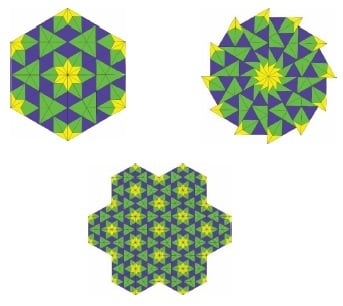
The prototiles obtained from the two-dimensional Delone faces are of three types of triangles with angles $\left(\frac{\pi }{3}, \frac{\pi }{3},\frac{\pi }{3}\right),$ $\left(\frac{\pi }{6}, \frac{\pi }{6},\frac{2\pi }{3}\right),\left(\frac{\pi }{6}, \frac{\pi }{3},\frac{\pi }{2}\right),$ represented by dark blue, yellow, and green triangles, respectively. Some patches of six-fold symmetric tilings by three triangles are shown in Figure 11, which follow from the substitution technique.

4.7. Prototiles from the Projection of the Voronoi Cell $V\left(0\right)$ of the Root Lattice $A_6$

The rhombic prototiles from the Voronoi cell $V\left(0\right)$ can be obtained from the formula $({(k_i)}_{\parallel },{(k_j)}_{\parallel })=\cos \left(\frac{2\pi \left(j-i\right)}{7}\right),i\ne j=1, 2,\dots ,7$. This would lead to three types of rhombi with angles $\left(\frac{\pi }{7},\frac{6\pi }{7}\right), \left(\frac{2\pi }{7},\frac{5\pi }{7}\right), \left(\frac{3\pi }{7},\frac{4\pi }{7}\right)$. There are numerous discussions on the seven-fold symmetric rhombic tiling with three rhombi. One particular construction is based on the cut and projection technique from a seven-dimensional cubic lattice [13]. See also the website of Professor Gerard t’ Hooft. A patch obtained by substitution technique is illustrated in Figure 12.

4.8. Projection of the Delone Cells of the Root Lattice $A_6$

The prototiles obtained from two-dimensional Delone faces are of four types of triangles with angles $\left(\frac{\pi }{7},\frac{\pi }{7},\frac{5\pi }{7}\right), \left(\frac{2\pi }{7},\frac{2\pi }{7},\frac{3\pi }{7}\right), \left(\frac{3\pi }{7},\frac{3\pi }{7},\frac{\pi }{7}\right), \mathrm{and} \left(\frac{\pi }{7},\frac{2\pi }{7},\frac{4\pi }{7}\right)$. The substitution tilings by the last three triangles are widely known as Danzer tiling. The number of prototiles obtained by projection here is the same as the tiles obtained from the tangents of the deltoid [41]. They have illustrated the patches involving only three of the triangles. In Figure 13, we illustrate a patch of sevenfold symmetric tiling comprising of all four triangles.

4.9. Prototiles from the Projection of the Voronoi CELL $V\left(0\right)$ of the Root Lattice $A_7$

The famous eightfold symmetric rhombic tiling by two prototiles is known as Amman–Beenker tiling [6]. Interestingly, enough we obtain the same prototiles from the projection of the Voronoi cell $V\left(0\right)$ of the root lattice $A_7$. The point group of the aperiodic tiling is the dihedral group $D_8$ of order 16 and the prototiles are generated by the pair of vectors satisfying the scalar product $({(k_i)}_{\parallel },{(k_j)}_{\parallel })=\cos \left(\frac{2\pi \left(j-i\right)}{8}\right),i\ne j=1, 2,\dots ,8$. We obtained two Amman–Beenker prototiles, one rhombus with angles $\left(\frac{\pi }{4},\frac{3\pi }{4}\right)$ and a square $\left(\frac{\pi }{2},\frac{\pi }{2}\right)$. A patch of aperiodic tiling is illustrated in Figure 14.

4.10. Projection of the Delone Cells of the Root Lattice $A_7$

Substituting $n=7$ in (13), we obtain five different triangular prototiles from the projection of the Delone cells of the root lattice $A_7$. Three of the prototiles are the isosceles triangles with angles $\left(\frac{\pi }{8},\frac{\pi }{8},\frac{6\pi }{8}\right)$, $\left(\frac{2\pi }{8},\frac{2\pi }{8},\frac{4\pi }{8}\right)$, $\left(\frac{3\pi }{8},\frac{3\pi }{8},\frac{2\pi }{8}\right)$ and the other two are the scalene triangles with angles $\left(\frac{\pi }{8},\frac{2\pi }{8},\frac{5\pi }{8}\right)$, $\left(\frac{\pi }{8},\frac{3\pi }{8},\frac{4\pi }{8}\right)$. So far as we know, no one has studied the tilings of the plane with these prototiles. Two patches of eightfold symmetric tilings with these prototiles are depicted in Figure 15.

4.11. Prototiles from Projection of the Voronoi Cell of the Root Lattice $A_{11}$

The 12-fold symmetric rhombic tiling has 3 prototiles of rhombuses with interior angles $\left(\frac{\pi }{6},\frac{5\pi }{6}\right)$, $\left(\frac{\pi }{3},\frac{2\pi }{3}\right)$, and $\left(\frac{\pi }{2},\frac{\pi }{2}\right)$. A patch of 12-fold symmetric tiling obtained by substitution technique is depicted in Figure 16.

4.12. Prototiles from the Projection of the Delone Cells of the Root Lattice $A_{11}$

The number of prototiles in this case is 12. As the rank of the Coxeter–Weyl group is increasing, the number of the triangular prototiles are also increasing. The 12 triangles are given as the set of integers $\left(n_1,n_2,n_3\right)$ defined in Section 3 as

$$\left(1, 1, 10\right), \left(1, 2, 9\right), \left(1, 3, 8\right), \left(1, 4, 7\right), \left(1, 5, 6\right), \left(2, 2, 8\right), \left(2, 3, 7\right), \left(2, 4, 6\right), \left(2, 5, 5\right),\left(3,3,6\right),\left(3,4,7\right),\left(4,4,4\right).$$

A patch of 12-fold symmetric tiling is depicted in Figure 17.

5. Concluding Remarks

Rhombic prototiles usually arise from projection of the higher dimensional cubic lattices $B_{n+1},$ because two-dimensional square faces project onto rhombuses and represent the local $2\left(n+1\right)$-fold symmetric rhombic aperiodic tilings of the Coxeter plane. Depending on the shift of the Coxeter plane, one may reduce the tilings to $\left(n+1\right)$-fold symmetric aperiodic tilings. The rhombic $\left(n+1\right)$-fold symmetric aperiodic tilings can also be obtained from the lattice $A_n,$ for the latter lattice is a sub-lattice of the lattice $B_{n+1}$. One may visualize that the lattice $B_{n+1}$ projects onto the lattice $A_n$ at first stage, as the Voronoi cell of the cubic lattice projects onto the Voronoi cell of the root lattice $A_n$. So, the classification of the rhombic aperiodic tilings of both lattices are the same. An advantage of the root lattice $A_n$ is that it can be tiled by the Delone cells with triangular two-dimensional faces. Projections of the Delone cells of the root lattice $A_n$ allow the classifications of the triangular aperiodic tilings. A systematic study of the projections of the Delone and Voronoi cells of the root and weight lattices of the simply laced ADE Lie algebras may lead to more interesting prototiles and aperiodic tilings. The present paper was concerned only with the aperiodic rhombic and triangular tilings of the root lattice exemplifying the 5-fold, 8-fold and 12-fold symmetric aperiodic tilings as they represent some quasicrystallographic structures.

References

- Shechtman, D.; Blech, I.; Gratias, D.; Cahn, J.W. Metallic phase with long-range orientational order and no translational symmetry. Phys. Rev. Lett. 1984, 53, 1951–1953. [Google Scholar] [CrossRef]
- Di Vincenzo, D.; Steinhardt, P.J. Quasicrystals: The State of the Art; World Scientific Publishers: Singapore, 1991. [Google Scholar]
- Janot, C. Quasicrystals: A Primer, 2rd ed.; Oxford University Press: Oxford, UK, 2012. [Google Scholar]
- Senechal, M. Quasicrystals and Geometry; Cambridge University Press: Cambridge, UK, 1995. [Google Scholar]
- Baake, M.; Grimm, U. Aperiodic Order, Volume 1: A Mathematical Invitation; Cambridge University Press: Cambridge, UK, 2013. [Google Scholar]
- Grünbaum, B.; Shephard, G.C. Tilings and Patterns; Freeman: New York, NY, USA, 1987. [Google Scholar]
- Penrose, R. The role of aesthetics in pure and applied mathematical research. Bull. Inst. Math. Appl. 1974, 10, 266–271. [Google Scholar]
- Penrose, R. Roger Penrose’s Pentaplexity article on aperiodic tiling. Eureka 1978, 39, 16–22. [Google Scholar]
- de Bruijn, N.G. Algebraic theory of Penrose’s non-periodic tilings of the plane. Nederl. Akad. Wetensch. Proc. Ser. 1981, 84, 38–66. [Google Scholar] [CrossRef]
- Duneau, M.; Katz, A. Quasiperiodic patterns. Phys. Rev. Lett. 1985, 54, 2688–2691. [Google Scholar] [CrossRef] [PubMed]
- Baake, M.; Joseph, D.; Kramer, P.; Schlottmann, M. Root lattices and quasicrystals. J. Phys. A Math. Gen. 1990, 23, L1037–L1041. [Google Scholar] [CrossRef] [Green Version]
- Chen, L.; Moody, R.V.; Patera, J. Fields Institute for Research in Mathematical Sciences Monographs Series 10; AMS: Providence, RI, USA, 1998; pp. 135–178. [Google Scholar]
- Whittaker, E.J.W.; Whittaker, R.M. Some generalized Penrose patterns from projections of n-dimensional lattices. Acta Crystallogr. Sect. A Found. Adv. 1988, 44, 105–112. [Google Scholar]
- Koca, M.; Koca, N.; Koc, R. Group-theoretical analysis of aperiodic tilings from projections of higher-dimensional lattices Bn. Acta Crystallogr. Sect. A Found. Adv. 2015, 71, 175–185. [Google Scholar]
- Boyle, L.; Steinhardt, P.J. Coxeter pairs, Ammann patterns and Penrose-like tilings. arXiv 2016, arXiv:1608.08215. [Google Scholar]
- Koca, N.O.; Koca, M.; Al-Siyabi, A. SU (5) grand unified theory, its polytopes and 5-fold symmetric aperiodic tiling. Int. J. Geom. Methods Mod. Phys. 2018, 5, 1850058. [Google Scholar] [CrossRef]
- Masáková, Z.; Patera, J.; Pelantová, E. Inflation centres of the cut and project quasicrystals. J. Phys. A Math. Gen. 1998, 31, 1443. [Google Scholar] [CrossRef]
- Meyer, Y. Algebraic Numbers and Harmonic Analysis, 1st ed.; North-Holland Pub. Co.: Amsterdam, The Netherlands, 1972. [Google Scholar]
- Lagarias, J.C. Meyer’s concept of quasicrystal and quasiregular sets. Commun. Math. Phys. 1996, 179, 365–376. [Google Scholar] [CrossRef]
- Moody, R.V. Meyer Sets and Their Duals, in The Mathematics of Long-Range Aperiodic Order, NATO ASI Series C; Kluwer Academic Publishers: Dordrecht, The Netherlands, 1997; Volume 489, pp. 403–441. [Google Scholar]
- Voronoi, G. Nouvelles applications des paramètres continus à la théorie des formes quadratiques. Deuxième mémoire. Recherches sur les parallélloèdres primitifs. J. Für Die Reine Und Angew. Math. 1908, 134, 198–287. [Google Scholar] [CrossRef]
- Voronoi, G. Part II of Voronoi (1908). J. Für Die Reine Und Angew. Math. 1909, 136, 67–181. [Google Scholar] [CrossRef]
- Delaunay, N.B. Izv. Sur la partition régulière de l’espace à 4 dimensions. Première partie. Akad. Nauk SSSR Otdel. Fiz. Mat. Nauk. 1929, 1, 79–110. [Google Scholar]
- Delaunay, N.B. Geometry of positive quadratic forms. Usp. Mat. Nauk. 1938, 3, 16–62. [Google Scholar]
- Delaunay, N.B. Geometry of positive quadratic forms. Part II. Usp. Mat. Nauk. 1938, 4, 102–164. [Google Scholar]
- Conway, J.H.; Sloane, N.J.A. Sphere Packings, Lattices and Groups; Springer: New York, NY, USA, 1988. [Google Scholar]
- Conway, J.H.; Sloane, N.J.A. Miscellanea Mathematica; Hilton, P., Hirzebruch, F., Remmert, R., Eds.; Springer: New York, NY, USA, 1991; pp. 71–108. [Google Scholar]
- Deza, M.; Grishukhin, V. Nonrigidity degrees of root lattices and their duals. Geom. Dedicate 2004, 104, 15–24. [Google Scholar] [CrossRef]
- Engel, P. Geometric Crystallography: An Axiomatic Introduction to Crystallography; Springer: Dordrecht, The Netherlands, 1986. [Google Scholar]
- Engel, P.; Michel, L.; Senechal, M. Lattice geometry. Preprint IHES /P/04/45. 1994. [Google Scholar]
- Moody, R.V.; Patera, J. Voronoi and Delaunay cells of root lattices: Classification of their faces and facets by Coxeter-Dynkin diagrams. J. Phys. A Math. Gen. 1992, 25, 5089–5134. [Google Scholar] [CrossRef]
- Koca, M.; Ozdes Koca, N.; Al-Siyabi, A.; Koc, R. Explicit construction of the Voronoi and Delaunay cells of W(An) and W(Dn) lattices and their facets. Acta Crystallogr. Sect. A Found. Adv. 2018, 74, 499–511. [Google Scholar]
- Ausloos, M.; Bartolacci, F.; Castellano, N.G.; Cerqueti, R. Exploring how innovation strategies at time of crisis influence performance: A cluster analysis perspective. Technol. Anal. Strateg. Manag. 2018, 30, 484–497. [Google Scholar] [CrossRef]
- Coxeter, H.S.M. Regular Polytopes, 3rd ed.; Dover Publications: New York, NY, USA, 1973. [Google Scholar]
- Grünbaum, B. Convex Polytopes; Wiley: New York, NY, USA, 1967. [Google Scholar]
- Humphreys, J.E. Cambridge Studies in Advanced Mathematics, Reflection Groups and Coxeter Groups; Cambridge University Press: Cambridge, UK, 1990; Volume 29. [Google Scholar]
- Michel, L. Bravais Classes, Voronoi Cells, Delone Cells, Symmetry and Structural Properties of Condensed Matter; Lulek, T., Florek, W., Walcerz, S., Eds.; World Scientific: Singapore, 1995; p. 279. [Google Scholar]
- Michel, L. Complete Description of the Voronoi Cell of the Lie Algebra An Weight Lattice. On the Bounds for the Number of d-Faces of the n-Dimensional Voronoi Cells, Algebraic Methods in Physics; Saint-Aubin, Y., Vinet, L., Eds.; Springer: Berlin/Heidelberg, Germany, 2001; pp. 149–171. [Google Scholar]
- Koca, M.; Koca, N.O.; Koc, R. Affine Coxeter group Wa (A4), quaternions, and decagonal quasicrystals. Int. J. Geom. Meth. Mod. Phys. 2014, 11, 1450031. [Google Scholar] [CrossRef]
- Carter, R.W. Simple Groups of Lie Type; John Wiley & Sons: New York, NY, USA, 1972; pp. 158–169. [Google Scholar]
- Nischke, K.P.; Danzer, L. A construction of inflation rules based on n-fold symmetry. Discret. Comput. Geom. 1996, 15, 221–236. [Google Scholar] [CrossRef]
Figure 1.
(a) Coxeter–Dynkin diagram of , (b) extended Coxeter–Dynkin diagram of .