An Optimization Framework for Codes Classification and Performance Evaluation of RISC Microprocessors

Abstract

Pipelines, in Reduced Instruction Set Computer (RISC) microprocessors, are expected to provide increased throughputs in most cases. However, there are a few instructions, and therefore entire assembly language codes, that execute faster and hazard-free without pipelines. It is usual for the compilers to generate codes from high level description that are more suitable for the underlying hardware to maintain symmetry with respect to performance; this, however, is not always guaranteed. Therefore, instead of trying to optimize the description to suit the processor design, we try to determine the more suitable processor variant for the given code during compile time, and dynamically reconfigure the system accordingly. In doing so, however, we first need to classify each code according to its suitability to a different processor variant. The latter, in turn, gives us confidence in performance symmetry against various types of codes—this is the primary contribution of the proposed work. We first develop mathematical performance models of three conventional microprocessor designs, and propose a symmetry-improving nonlinear optimization method to achieve code-to-design mapping. Our analysis is based on four different architectures and 324,000 different assembly language codes, each with between 10 and 1000 instructions with different percentages of commonly seen instruction types. Our results suggest that in the sub-micron era, where execution time of each instruction is merely in a few nanoseconds, codes accumulating as low as 5% (or above) hazard causing instructions execute more swiftly on processors without pipelines.

1. Introduction

Reduced Instruction Set Computer [1], or RISC for short, has seen tremendous advancement over the last four decades. Starting from a simple MIPS [2], RISC processors dominated in smartphones and tablet computers [3], and have recently been used in a supercomputer named Sunway TaihuLight [4], comprising ten million cores—making it the fastest supercomputer in the world (https://www.top500.org/lists/2017/11/). It has also been reported (https://www.theverge.com/2017/3/9/14867310/arm-servers-microsoft-intel-compute-conference) that Microsoft (R) has recently unveiled its new Advanced RISC Machines (ARM) server designs, thereby beginning to challenge Intel’s dominance of the industry.

Earlier versions of the RISC processor did not have pipeline stages; instead each instruction was executed exactly in a clock cycle in a mutually exclusive manner—therefore, the name Single Cycle Processor (SCP) [5]. The performance limitations of the SCP were addressed in the advanced versions, which were based on multicycle execution of each instruction, and later followed by incorporation of pipelining, in which multiple instructions could be executed in parallel [6]. Since pipelining was supposed to guarantee massive throughputs, it became the de facto architecture for most modern processors [7,8], video coders/decoders [9,10], and crypto systems [11,12], to name a few. Unfortunately, it was completely overlooked that there might be situations in which the older variants, SCP and Multicycle Processors (MCP), could outperform the Pipelined Processors (PiP). One such situation could be the way an assembly language program was written. It is often the case that a particular instruction causes hazards that are not suitable for the PiP, and rather executes more swiftly on an SCP. The greater the hazardous instructions in the assembly language code, the more suitable the simpler variant shall be. Therefore, in this work we try to analyze the given assembly language code first, before making choice of the processing architecture.

While proceeding miniaturization has allowed integration of billions of transistors on a chip [13], and resources are readily available in abundance, excessive power consumption, rather than size, in digital circuits, such as microprocessors, is becoming a much graver concern. In our context, fabricating the three variants of RISC processors on a single chip, and then making a choice between them according to the assembly language code should resolve the problem, however, only at the expense of increased dynamic power consumption. Luckily, there exists a technique called Dynamic Partial Reconfiguration (DPR) [14,15], which allows real-time reconfiguration of a part of the circuit, while another part is still in execution. Therefore, it is possible to generate partial bit files for each variant, keep them in the reconfigurable memory of the chip, and download one of them at a time on to the system according to the code being executed without having to stop or restart the whole system. Importantly, this will constrain the power consumption only to the active processor type. This, however, was only possible if we were first able to classify the assembly language codes according to their suitable processor variant, using some classification method [16].

In this work, we first develop a mathematical performance model for each of the three design paradigms (SCP, MCP, and PiP) using a set of commonly seen instructions. By subjecting these models to a symmetry-targeted monotone optimization technique, we determine which class of variants does a given assembly language code, with a certain percentage of each instruction, suit the best. We carry out our analysis on 8-bit, 16-bit, 32-bit and 64-bit MIPS processors, where the number of instructions in each code varies between 10 and 1000. Our confidence stems from 324,000 assembly language codes, each comprising different percentage of each instruction, per processor architecture. Please note that it is beyond the scope of this work to present design and operation of the dynamically reconfigurable (DR) processor; instead, we try the use of each design paradigm according to the given assembly language program by comparing their execution times with each other, and advocating the DR processor that promises performance symmetry in every circumstance for the given code in run time. The major contributions of this work, therefore, are as follows:

• Performance modeling of three conventional processor types for commonly seen instructions
• Classification of assembly language codes for code-to-processor mapping using an optimization technique based on symmetry-improving nonlinear transformation

We conclude that in the sub-micron era, where execution time of each instruction is merely in a few nanoseconds, codes accumulating as low as 5% hazard causing instructions execute more swiftly on processors without pipelines. Our results shall be vital in the context of multi-processor systems-on-chip and chip multi-processors, where one more efficient function unit is replaced by multiple simpler variants in order to attain increased throughputs by exploiting parallelism, yet, keeping the complexity of the system unaffected or marginally increased [17]. To the best of our knowledge, there is no framework available in the literature that could be considered equivalent to the proposed one.

The rest of the paper is organized as follows: In Section 2, we review some of the recent applications of DPR, and introduce our basic processors and the instructions that they support. A mathematical performance model for each processor is presented in Section 3, which is subsequently used to define three optimization problems and their solutions in Section 4—this is the main contribution, which also comprises our proposed research methodology. Section 5 presents results and evaluation, and a few sample assembly language codes that suit SCP more than the PiP according to the proposed formulation. We conclude the paper in Section 6.

2. Background and Related Work

2.1. Dynamic Partial Reconfiguration

Dynamic Partial Reconfiguration (DPR) is a technique used to update the logic blocks dynamically while a part of the system is still in execution. The DPR allows the designers to generate partial bit files, which can be implemented and downloaded into the system without the need for system shutdown or restart. As a result, the system functionality is upgraded in runtime without any interruption.

The digital systems using the concept of DPR can be categorized into two: a static non reconfigurable part of the design, and runtime reconfigurable part. The former uses the generated full bit stream of the design downloaded into the system at boot time, whereas, the runtime reconfigurable part of the design may comprise several independent reconfiguration regions. These regions have a flexibility to be reconfigured in runtime by downloading the generated partial bit streams without affecting the functionality of the static non reconfigurable part [18].

The system reconfiguration time for a specific reconfigurable region using the DPR concept is proportional to the partial bit stream size. This timing constraint is a key factor in determining the worst case execution time of the design, and is considered as a time overhead each time the system is reconfigured [19].

The major advantage of DPR is that it enhances design flexibility and minimizes the design area. This promising feature can be used to implement numerous system applications used in diverse engineering fields, such as signal, image and video processing [20]. The concept of DPR is also used for database management. An energy aware SQL query acceleration method using DPR concept on XILINX ZYNQ platform has been presented [21], and a significant improvement in energy consumption as compared to X86 based system is shown. Another diverse field recently using the DPR concept is the evolution of artificial neural networks on FPGA. A very unique method to address fault problems in synapses of spiking neural networks using astrocyte regulation, inspired by brain recovery process is demonstrated [22].

The DPR concept may also be used in applications and systems where latency is considered as one of the prime factors to determine the system’s performance. Various processor design styles [23,24] may be implemented in runtime that will have a significant impact in terms of execution time—thereby on performance of a specific program, as discussed in this work.

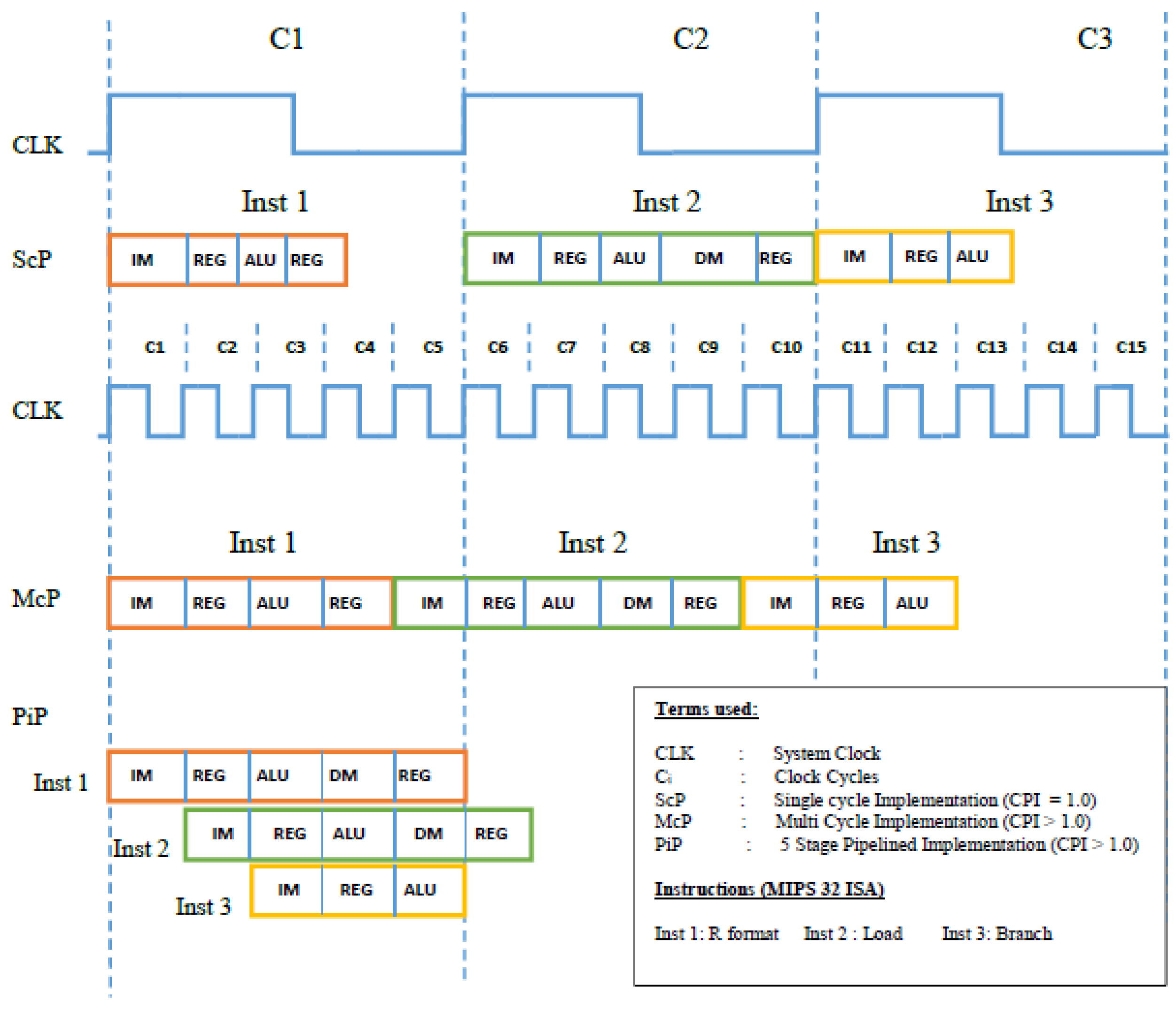
2.2. Processor Design Styles

RISC architectures, especially when used in industrial embedded systems applications, generally follow one of the three design paradigms. These include single cycle, multi cycle, and pipelined architectures. MIPS [2] is still considered as the benchmark architecture lying in core of most of the modern RISC processors. This is why, in this work we restrict our analysis to MIPS, but we try to keep our assumptions and methodology as general as possible. In what follows, we briefly present the design and operation of each of the three design paradigms in turn.

2.2.1. SCP

As the name suggests, an SCP is guaranteed to execute each instruction in the instruction set architecture (ISA) exactly in one clock cycle, where each instruction is supposed to access various function units constituting the processor. These units typically include instruction/program memory, register file, arithmetic and logic unit (ALU), data memory, and control unit (CU), each with a different latency. Since each instruction may access a different set of units in a unique sequence, the execution time for each instruction will be different, and naturally, the clock cycle time should be long enough to accommodate the slowest instruction (with the largest execution time).

2.2.2. MCP

An MCP executes each instruction in more than one clock cycles, depending upon the number of function units it accesses. Therefore, a longer instruction will consume several clock cycles while executing, whereas the shorter instructions will consume less. The clock cycle is just long enough to accommodate only one function unit—naturally it must be the slowest function unit to dictate the clock cycle time.

Since only one function unit is supposed to work in each clock cycle, it has become a convention to name each clock cycle after the function unit in charge of that clock cycle: Instruction Fetch (read the program memory), Decode (read the operands in the register file, and CU decodes OP-Code), Execute (ALU either performs the desired operation or computes physical address to read/write the data memory), Memory Access (read/write the data memory or register write for some instructions), and Write-back (data read from memory is written on to a register).

2.2.3. PiP

The pipelining technique divides the datapath into n pipeline stages, named exactly like clock cycles on the MCP, where each stage consists of exactly one function unit. These types of processors are supposed to achieve higher throughput than the previous ones, by ensuring that no pipeline stage remains idle at any point in time. Instead, n instructions can form a queue in the datapath, while each occupies a pipeline stage simultaneously, thereby exploiting parallelism. Each stage, m, needs to be synchronized with $m-1$ and $m+1$ neighboring stages, otherwise data from one stage may interfere the operation of the next. Understandably, the clock cycle time is determined according to the slowest pipeline stage, which ensures proper synchronization between the pipeline stages. Figure 1 presents timing diagram for the three variants on random instructions.

A drawback associated with PiP is the existence of structural, data, and control hazards [25]. Without going into details of each of those, it is essential mentioning that a few of data and control hazards require stalling the pipeline, inserting a bubble, or flushing a pipeline register for correct operation. In either case, each of such hazards will incur delay of a time slot on top of the normal execution time of the instruction causing hazard. In case the code to be executed comprises several instructions causing hazards, the execution time may exceed that of the SCP or MCP, making latter an appropriate choice specifically for this code. However, in integrated circuits that are not dynamically reconfigurable, one has to bear this undesired overhead.

2.2.4. Instruction Types

As there can be infinitely many types of instructions, each accessing the function units infinitely many times, it is usually reasonable to restrict the analysis to a specific instruction types. There are five basic types of instructions supported by, more or less, every microprocessor. These include:

• Register (R)—Format, in which the source as well as the destination operands belong to the register file.
• Load Word (LW), in which a data item is fetched from data memory and loaded in a register. The physical address is formed by adding a base address, which comes from a register, to an offset encoded in the instruction.
• Store Word (SW), in which the data item is read from a register and moved into a location on data memory, where physical address is computed in the same manner as for LW.
• Branch, in which flow of the program changes based on a condition: instead of fetching the next sequential instruction, instruction present at the target address is fetched on to the processor. The condition is usually checked by the ALU or a comparator on operands from register file. Please note that until the condition is checked (say found true), at least one instruction, usually the one next in line sequentially, may have already been fetched into the pipeline—leading to a control hazard in case of PiP. It is called a hazard since the incorrectly fetched instruction needs to be flushed out of the pipeline before it carries out an erroneous activity, e.g., a memory read/write or a register write.
• Jump, in which flow of the program changes unconditionally. Likewise for the branch instruction in a PiP, Jump will require flushing the pipeline at least once, before the correct instruction is fetched.

Although there are several variants of these instructions, we will do the formulation only for the basic instructions enumerated above in the following section. Our objective is to estimate the execution times for different instruction mix, i.e., for assembly language codes comprising varying percentages of the selected instructions on each processor. The execution time of a program comprising I instructions, in general, is given as Equation (1).

$$E=I\times CPI\times CLK$$

(1)

where CPI refers to number of clock cycles per instruction, and $CLK$ is clock cycle time. The formulation in the next section will enable us to classify codes according to their appropriateness for each type of processor. This classification requires optimization of the performance models, which can be achieved by various methods—generally categorized into deterministic and stochastic optimization methods—discussed next.

2.3. Optimization Methods

The stochastic optimization methods are used in situations where data, for some reason, are not known in advance, or at least not known with certainty [26]. Bio-inspired techniques, over the years, have gained attention in solving such optimization problems, which incorporate the uncertainty into the model; a few recent examples include [27,28,29,30]. Advantages of these techniques are best leveraged if the solution search space is not well-structured and understood. Naturally, their latency, in terms of convergence rate, will be substantial, yet they are known to be best-effort techniques, since their objective is to obtain a near-optimal solution [31,32].

As shall be seen in Section 3 and Section 4, the mathematical models that we have developed, and the optimization problem at hand, hardly have an uncertainty involved, due to which the solution search space is nicely structured as well. This relieves us from employing much more complex stochastic optimization, and turn to much simpler solutions for deterministic optimization problems. The mathematical model has yielded a nonlinear optimization problem, for which we have made use of symmetry-targeted nonlinear transformation [33] (discussed later in Section 4), followed by a widely adopted method of linear programming. An optimization problem is said to be linear programming problem if its objective function, decision variables and constraints are all linear functions. Such problems are typically handled using the simplex method, in which the decision variables are iteratively updated to yield the most feasible solution (optimal objective function) [34].

While, the details on the proposed optimization method will be presented in Section 4, in what follows, we present modeling of the three processor types first.

3. Mathematical Modeling

3.1. Preliminary Assumptions

Let $\mathbb{L}=\{{\alpha }_i,{\alpha }_{i+1},\cdots ,{\alpha }_{i+4}\}$ be the set of latencies for the major function sequences involved in execution of a typical instruction on a processor implementing Harvard architecture. Here ${\alpha }_i$, $\forall i\in \mathbb{N}$ and $i<6$, represents IM access, RF access, ALU operation, DM access, and CU operation respectively. For simplicity, we are assuming that ${\alpha }_{RFread}={\alpha }_{RFwrite}$ and similarly ${\alpha }_{DMread}={\alpha }_{DMwrite}$. Also, it is realistic to assume that ${\alpha }_{CU}<{\alpha }_{RFread}$. Without the loss of generality, let us assume the instruction mix is as follows: $Branch=x_1\%$, $Jump=x_2\%$, $R-Format=x_3\%$, $Load=x_4\%$, and $Store=x_5\%$. Considering the fact that each variant of the processor will suffer the same penalty, we also assume the probability of read/write miss to be zero.

3.2. Formulation for SCP

The execution time for each type of instruction is formulated as follows in

Table 1. Execution times ($E_i$) for each type of instruction on Single Cycle Processor.

Instruction	Expression
$Branch$	$E_1$	=	${\sum }_{i=1}^3{\alpha }_i$
$Jump$	$E_2$	=	${\alpha }_1+{\alpha }_5$
$R-Format$	$E_3$	=	$E_1+{\alpha }_2$
$Load$	$E_4$	=	$E_1+{\alpha }_2+{\alpha }_4$
$Store$	$E_5$	=	$E_4-{\alpha }_2$

:

The clock cycle time for this type of processor $(CL{K}_S)$ is given by Equation (2).

$$CL{K}_S=ma{x}_{i=1}^5{E}_i$$

(2)

The execution time $(E_S)$ of the given code, also termed as User CPU Time is given by Equation (3):

$$E_S=I\times CL{K}_S$$

(3)

where I refers to the number of instructions in the given code; note that the CPI for SCP is 1. It is widely understood that by employing pausible clocks [25], each instruction may be executed by a different clock cycle, and therefore the performance of such processors may be significantly improved. In that case, Equation (2) will not hold; we will have to compute the average clock cycle time, considering different $E_i$—let us denote it with $CL{K}_{SV}$, given by Equation (4).

$$CL{K}_{SV}=\frac{1}{100}(x_1{E}_1+x_2{E}_2+x_3{E}_3+x_4{E}_4+x_5{E}_5)$$

(4)

Similarly, Equation (3) for the execution time for this variant will now have to be modified accordingly, given by Equation (5).

$$E_{SV}=I\times CL{K}_{SV}$$

(5)

3.3. Formulation for MCP

In multicycle processors, the clock cycle time, $CL{K}_M$ is determined by the slowest function unit, and each instruction may consume multiple clock cycles to execute, as shown in

Table 2. Clock Cycles $(C_i)$ to execute each type of instruction on Multicycle Processor.

Instruction	Number of Clock Cycles
$Branch$	$C_1$	=	3
$Jump$	$C_2$	=	3
$R-Format$	$C_3$	=	4
$Load$	$C_4$	=	5
$Store$	$C_5$	=	4

. Its execution time, $E_M$, is given by Equation (6).

$$E_M=I\times CP{I}_M\times CL{K}_M$$

(6)

where $CP{I}_{av}$ and $CL{K}_M$ are given by Equations (7) and (8) respectively.

$$CP{I}_M=\frac{1}{100}(3x_1+3x_2+4x_3+5x_4+4x_5)$$

(7)

$$CL{K}_M=ma{x}_{i=1}^5{\alpha }_i$$

(8)

Once again, pausible clocking may be employed to reduce $CL{K}_M$, but this time the improvement will not be notable. While clock cycles 1 and 4, requiring memory accesses, should be according to Equation (8), clock cycles 3 and 5 should be dictated by ${\alpha }_3$ and ${\alpha }_2$ respectively, and clock cycle 2 should depend upon the condition $max({\alpha }_2,{\alpha }_3)$ due to the overlap of register file access and ALU operation. The average $CL{K}_{MV}$ in this case will be computed as Equation (9).

$$CL{K}_{MV}=\frac{1}{5}({\alpha }_2+{\alpha }_3+max({\alpha }_2,{\alpha }_3)+2{\alpha }_4)$$

(9)

3.4. Formulation for PiP

Unfortunately, formulation for the PiP is not that simple. The data hazards that require stalling the pipeline tend to add an extra time slot; so the more the hazards, the more the cycles will be wasted. Similarly, the control hazards also increase the latency by one time slot, for example, the Jump instruction will unconditionally cost an extra time slot, and Branch instructions, if true, will do the same. All this needs to be accounted for while computing the exact CPU time for the given code.

Equation (8) holds true for this processor too; so $CL{K}_P=CL{K}_M$. Other than the time slots wasted due to conditions discussed above, the execution time is computed as follows: the first instruction consumes n time slots for n-stage deep pipeline, while each of the following instructions is executed in one time slot. This is given by Equation (10).

$$E_{P\_base}=n\times CL{K}_P+(I-1)\times CL{K}_P$$

(10)

As far as additional time slots due to hazards are concerned, each case needs to be addressed independently. We have mentioned already that each Jump instruction will unconditionally cost an extra time slot. Therefore, $x_2\%$ Jump instructions will add an overhead of $0.01\times x_2\times I$ clock cycles in the overall execution time. Likewise, for Branch instructions that turn out to be true, $0.01\times x_1\times I$ clock cycles will be added. However, in this case, the probability of Branch being true must be considered as well. Since this is nondeterministic, we assume a fair decision, i.e., $50\%$ branches will be true.

The last case that remains is of a data hazard that forces a stall in the pipeline, i.e., a Load instruction followed by a dependent instruction. Recall that any instruction, other than Jump, may cause a data hazard with the preceding Load instruction with some probability deduced from the total number of registers in the register file. Furthermore, the dependency may exist between the target register ($\$Rd$) of the Load and any of the two source operands ($\$Rs$) or ($\$Rt$) of the following instruction. The probability of a hazard due to matching of ($\$Rd$) with any one of ($\$Rs$) and ($\$Rt$) is given by Equation (11)

$$Prob\_hazard=\frac{2R_{max}-1}{R_{max}^2}$$

(11)

where $R_{max}$ is the total number of registers in the register file. Since a hazard cannot be caused by a Jump instruction, the probability for being a hazardous instruction is important, and is given by Equation (12).

$$Prob\_hazardous\_inst=\frac{x_4}{100}(1-\frac{x_2}{100})\times I$$

(12)

Taking into account the cases for control and data hazards discussed above, the modified execution time for the PiP is given by Equation (13).

$$E_P=E_{P\_base}+I\times CL{K}_P[\frac{1}{2}\frac{x_1}{100}+\frac{x_2}{100}+\frac{x_4}{100}(1-\frac{x_2}{100})(\frac{2R_{max}-1}{R_{max}^2})]$$

(13)

Substituting Equation (10) into Equation (13) and performing simplification for $n=5$, simplified $E_P$ is given by Equation (14)

$$E_{P\_simp}=4CL{K}_P+ICL{K}_P[1+\frac{1}{2}\frac{x_1}{100}+\frac{x_2}{100}+\frac{x_4}{100}(1-\frac{x_2}{100})(\frac{2R_{max}-1}{R_{max}^2})]$$

(14)

3.5. Estimating Worst and Best Case Performance

Our objective is to maximize and minimize $E_{ϵ}$ for estimating worst and best case performance of each processor type, where $ϵ\in \{S,SV,M,P\_simp\}$ corresponding to Equations (3), (5), (6), and (14) respectively. For a given I, $E_S$, Equation (3), is a constant value; therefore, $E_{Smax}=E_{Smin}$− making this type of processor suitable only for codes comprising very few instructions.

For the variant of SCP given by Equation (5), $E_{SVmax}\Rightarrow CL{K}_{SVmax}$, and $E_{SVmin}\Rightarrow CL{K}_{SVmin}$ where $CL{K}_{SV}$ is given in Equation (4). Since $E_4>E_i\forall i\in \{1\cdots 5\}:i\ne 4$, and $E_2<E_i\forall i\in \{1\cdots 5\}:i\ne 2$, from Figure 4, and ${\sum }_{i=1}^5{x}_i=100$, $CL{K}_{SVmax}$ and $CL{K}_{SVmin}$ are given by Equations (15) and (16) respectively.

$$CL{K}_{SVmax}=E_4//x_4=100,x_1=x_2=x_3=x_5=0$$

(15)

$$CL{K}_{SVmin}=E_2//x_2=100,x_1=x_3=x_4=x_5=0$$

(16)

For the case of MCP, given by Equation (6), the worst case performance corresponds to $E_{Mmax}\Rightarrow CP{I}_{Mmax}$, Equation (7). Similarly, the best case performance requires minimizing Equation (7). It is understandable that $CP{I}_{Mmax}=5$ for $x_4=100$ and $x_1=x_2=x_3=x_5=0$, and $CL{K}_{Mmax}={\alpha }_4$, since we usually assume data memory access to be the slowest function step. Similarly, $CP{I}_{Mmin}=3$ for $x_1=100$ or $x_2=100$.

For the case of PiP, the instruction mix dictates the best and worst case performance. $E_{P\_simp}$, Equation (14), is modified as following, Equations (17) and (18) to obtain $E_{P\_simp\_min}$ and $E_{P\_simp\_max}$ accordingly.

$$E_{P\_simp\_min}=4CL{K}_P+ICL{K}_P//for{x}_1=x_2=x_4=0$$

(17)

$$E_{P\_simp\_max}=4CL{K}_P+2ICL{K}_P//for{x}_2=100,x_1=x_4=0$$

(18)

3.6. Discussion

Based on the formulation presented above, a few observations may be conveniently made:

• The second variant of SCP performs much better for shorter instructions, such as Jump and Branch. So, the more the shorter instructions in the code, the more suitable the SCP should be.
• The performance of the PiP entirely depends upon instruction mix: if there is no hazardous instruction, this type will stand out as the best. However, the more the control hazards in the code, the larger the execution time will be. Furthermore, $CL{K}_P$ is dictated by the slowest function step, which means the larger the difference between the latencies of function units, the larger the $CL{K}_P$ will be in comparison to $CL{K}_{SV}$.
• In terms of performance, it is difficult for the MCP to beat the other two. The reason for this observation is its $CP{I}_M$ of 3 for shorter instructions, which suit the SCP more. On the other hand, the PiP will outclass it for longer instructions.

So, we have to optimize instruction mix, and latencies of the function units to determine regions where the SCP will outperform the PiP. Based on our results, the compilers will be able to determine the better processing platform for the given application in run-time.

4. Problem Statement and Proposed Optimization

4.1. Problem Statement & System Model

The first objective, optimization problem ($O{P}_1$), of the proposed work is given by Equation (19)

$$O{P}_1:\underset{\mathbf{x}}{min}{E}_{P\_simp}-E_{SV}$$

(19)

subject to:

• $C_{11}:E_{P\_simp}-E_{SV}>0$
• $C_{21}:{\sum }_{i=1}^5{x}_i=100$
• $C_{31}:0\le$x$\le 100$

where $E_{P\_simp}$ and $E_{SV}$ are given by Equations (5) and (14) respectively in terms of decision variables: x $=\{x_i\}\forall i\in \{1\cdots 5\}$, and $C_{11}to{C}_{31}$ are the constraints that the optimized solution must satisfy. The inputs to our system include two types of microprocessors that have five types of instructions in their ISA, and we assume 8, 16, 32, and 64 bit architectures, which usually support eight, sixteen, thirty two, and sixty four general purpose registers respectively. Another input is latency of the function units, ${\alpha }_i\forall i\in \{1\dots 5\}$. Please note that ${\alpha }_i\approx {\alpha }_4$ are technology dependent—for DDR(2−4) SDRAM. The number of instructions in the given code I is the final input.

Using Equations (14) and (5), and following some trivial simplification and rearrangement, $E_{P\_simp}-E_{SV}$ may be written as Equation (20), which may further be simplified to Equation (21).

$$E_{P\_simp}-E_{SV}=CL{K}_P(I+4)+\sum _{i=1}^5({\varrho }_{i}I)x_i+({\varrho }_{6}I)x_2{x}_4$$

(20)

where

• ${\varrho }_1=0.5CL{K}_P-E_1$
• ${\varrho }_2=CL{K}_P-E_2$
• ${\varrho }_3=-E_3$
• ${\varrho }_4=CL{K}_P(\frac{2R_{max}-1}{R_{max}^2})-E_4$
• ${\varrho }_5=-E_5$
• ${\varrho }_6=CL{K}_P(\frac{1-2R_{max}}{R_{max}^2})$

$$E_{P\_simp}-E_{SV}=({\varrho }_{6}I)x_2{x}_4+U(\mathbf{x})$$

(21)

Clearly, the product $x_2{x}_4$ makes our objective function a nonlinear programming (NLP) problem [35]. Solving NLP problems requires nonconvex to convex relaxation [36], i.e., symmetry-improving nonlinear transformation by relaxing the bounds, in order to eradicate possibility of getting multiple local minima. Shachar et al. [37] demonstrated that variable transformation with symmetric distribution (close to Gausian) helps in achieving linearity in the inter-variable relationship. Although it is often not expedient to achieve symmetry due to irregular structure of the variable, yet, it proves advantageous. We, therefore, introduce a variable, Z, as a first step to linearize Equation (21), leading to $O{P}_2$, given by Equation (22).

$$O{P}_2:\underset{\mathbf{x},Z}{min}Z$$

(22)

subject to:

• $C_{12}:Z\ge 0$
• $C_{22}:({\varrho }_{6}I)x_2{x}_4+U(\mathbf{x})=Z$
• $C_{32}:{\sum }_{i=1}^5{x}_i=100$
• $C_{42}:0\le \mathbf{x}\le 100$

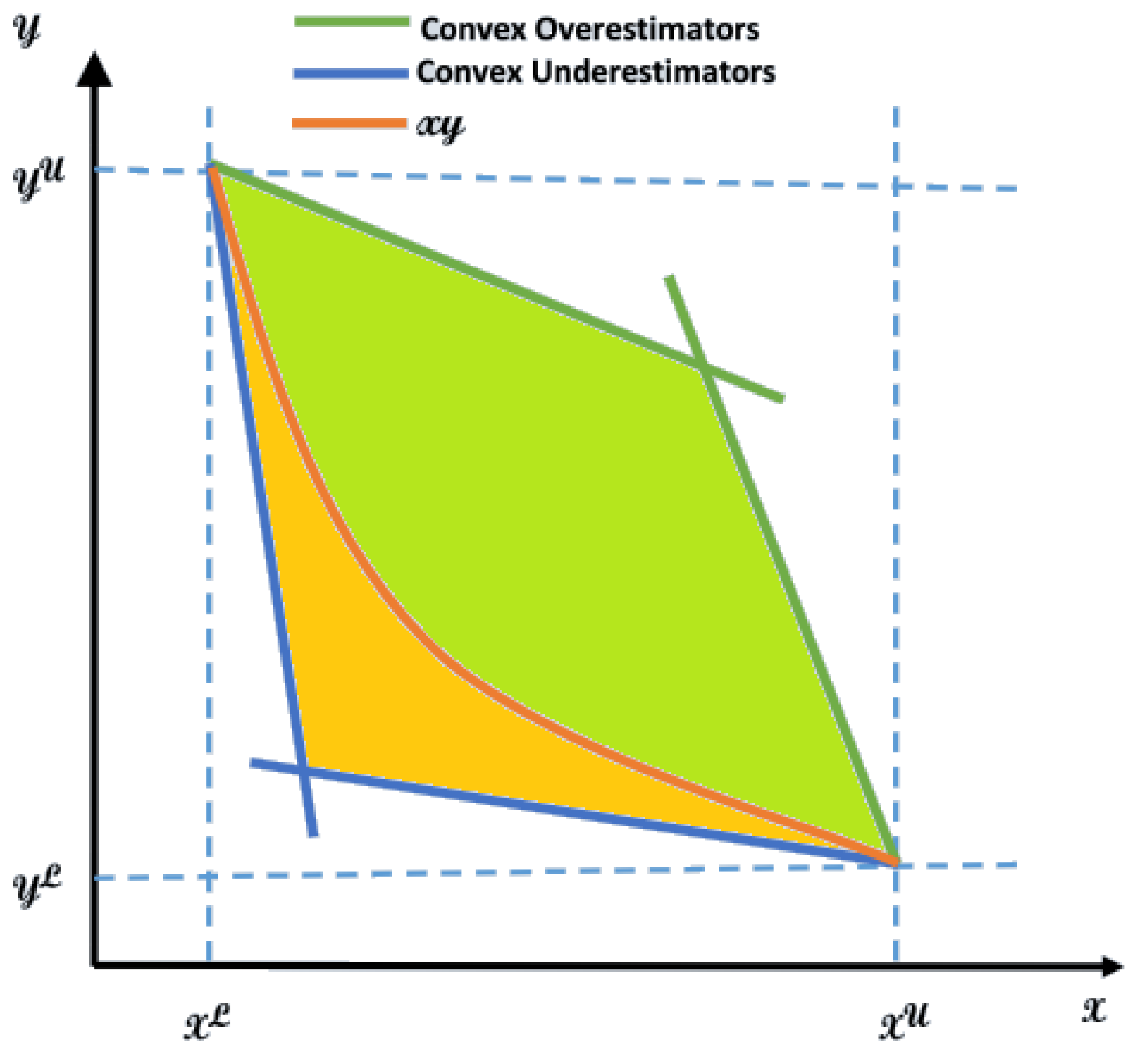
4.2. Convex Relaxation using McCormick’s Envelopes

Although nonlinear to linear transformation reduces computational complexity, the obtained solution will only be optimal to the relaxed objective function, rather than to the original. Therefore, relaxation only provides a lower bound closer to the actual optimal solution, while the upper bound may then be obtained by solving the original nonconvex problem using solutions acquired from the relaxed optimization [38]. Please note that tighter relaxation on bounds will yield solutions closer to the optimal solution. McCormick’s Envelopes provides such relaxation, i.e., it retains convexity by keeping tight bounds [39]. Figure 2 presents under and over estimators in McCormick’s envelopes for a nonlinear function $w=xy$, where U and L stand for upper and lower bounds respectively.

For solving $O{P}_2$ using McCormick’s envelopes, recall that $x_2{x}_4=\frac{Z-U(\mathbf{x})}{{\varrho }_{6}I}$ from $C_{22}$. Then, the under and over estimators are given by

• $\frac{Z-U(\mathbf{x})}{{\varrho }_{6}I}\ge x_2^L{x}_4+x_2{x}_4^L-x_2^L{x}_4^L$
• $\frac{Z-U(\mathbf{x})}{{\varrho }_{6}I}\ge x_2^U{x}_4+x_2{x}_4^U-x_2^U{x}_4^U$
• $\frac{Z-U(\mathbf{x})}{{\varrho }_{6}I}\le x_2^L{x}_4+x_2{x}_4^U-x_2^L{x}_4^U$
• $\frac{Z-U(\mathbf{x})}{{\varrho }_{6}I}\le x_2^U{x}_4+x_2{x}_4^L-x_2^U{x}_4^L$

where $x_2^L\le x_2\le x_2^U$, $x_4^L\le x_4\le x_4^U$ and lower and upper bounds are given above by $C_{31}$ and $C_{42}$. With these new linear constraints, we are able to transform a nonlinear problem, Equation (22), into a linear optimization problem, $O{P}_3$, as follows:

$$O{P}_3:\underset{\mathbf{x},Z}{min}Z$$

(23)

subject to:

• $C_{13}:Z\ge 0$
• $C_{23}:{\sum }_{i=1}^5{x}_i=100$
• $C_{33}:0\le \mathbf{x}\le 100$
• $C_{43}:\frac{Z-U(\mathbf{x})}{{\varrho }_{6}I}\ge 0$
• $C_{53}:\frac{Z-U(\mathbf{x})}{{\varrho }_{6}I}\ge 100(x_2+x_4)-10000$
• $C_{63}:\frac{Z-U(\mathbf{x})}{{\varrho }_{6}I}\le 100x_2$
• $C_{73}:\frac{Z-U(\mathbf{x})}{{\varrho }_{6}I}\le 100x_4$

which may be solved using conventionally used interior point [40] or simplex method of linear programming [34].

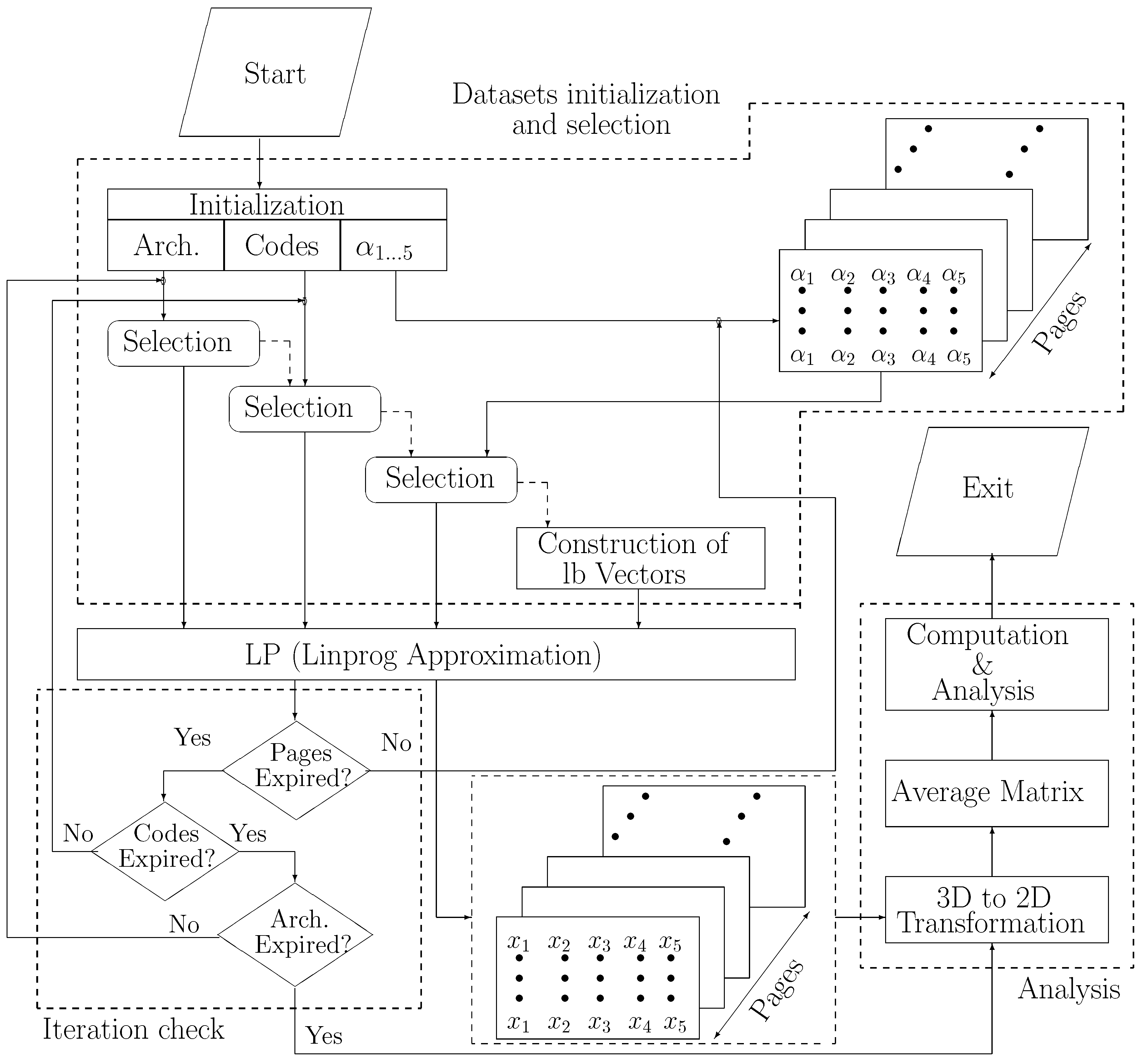
4.3. Proposed Methodology and Algorithm

Figure 3 summarizes our research methodology. We initialize the system by randomly choosing various architectures (Arch., $\Gamma$), various codes of different lengths ($\mathbb{C}$), and a large set of ${\alpha }_i$ arranged in pages ($\mathfrak{F}$) as shown. Each round of execution makes a selection from each of these inputs, and constructs a vector of lower bound (lb) on each type of instruction, except for Jump. To determine confidence intervals for feasible solutions, at each iteration we increment lb on each type of instruction by a certain number − details will be given in the evaluation section. By doing so, the optimizer ($\mathbb{L}\mathbb{P}$) is forced to find a solution in higher percentages of Jump instructions − providing a wide coverage of feasible solutions. The proposed Algorithm 1 continues to run until the number of pages ($P_{max}$), codes ($C_{max}$), and architectures ($R_{max}$) have expired. During each round of execution, a page of feasible solutions, comprising percentage of each instruction, is recorded. Upon termination, average percentage of each instruction ($\mathbb{A}$), across the pages, is computed via 3D to 2D transformation ($T_{mat}$), following which in depth analysis of the results is carried out. This analysis mainly involve observing ratios of Jump and Branch to rest of the instructions in feasible solutions ($B_2^R$, $J_2^R$). The objective of this analysis is to determine contribution of the former two instructions in a code that should satisfy $O{P}_3$, i.e., the cases where SCP performs better than the PiP.

Algorithm 1: Proposed Algorithm.

5. Evaluation and Sample Codes

To verify the proposed approach, we have modeled the linear optimization problem, given by Equation (23), using the methodology described in Section 4.3 in MATLAB. The linear programming solver that we have used is linprog, which uses dual-simplex method to generate an optimal solution. Our samples and datasets are initialized as discussed in the following subsection.

5.1. Data Initialization

For evaluating and comparing performances of SCP and PiP with each other, we have chosen the following vectors:

• $R_{max}=\{8,16,32,64\}$—representing four different architectures
• ${\alpha }_1={\alpha }_4=\{1,2,3,4,5,6,7,8\}$—representing propagation delays of function modules. The vector is chosen, as such, for simplicity, since ${\alpha }_i,\forall i\in \{1,4\}$, is technology dependent, and may lie in the range $\{1-8\}ns$ for recent technology nodes. Here, ${\alpha }_2$ and ${\alpha }_3$ will always be smaller than the other two, and are randomly selected.
• $I=\{10,100,500,1000\}$—representing four different assembly language code lengths. These values will give us a confidence interval for performance of each processor’s variant.
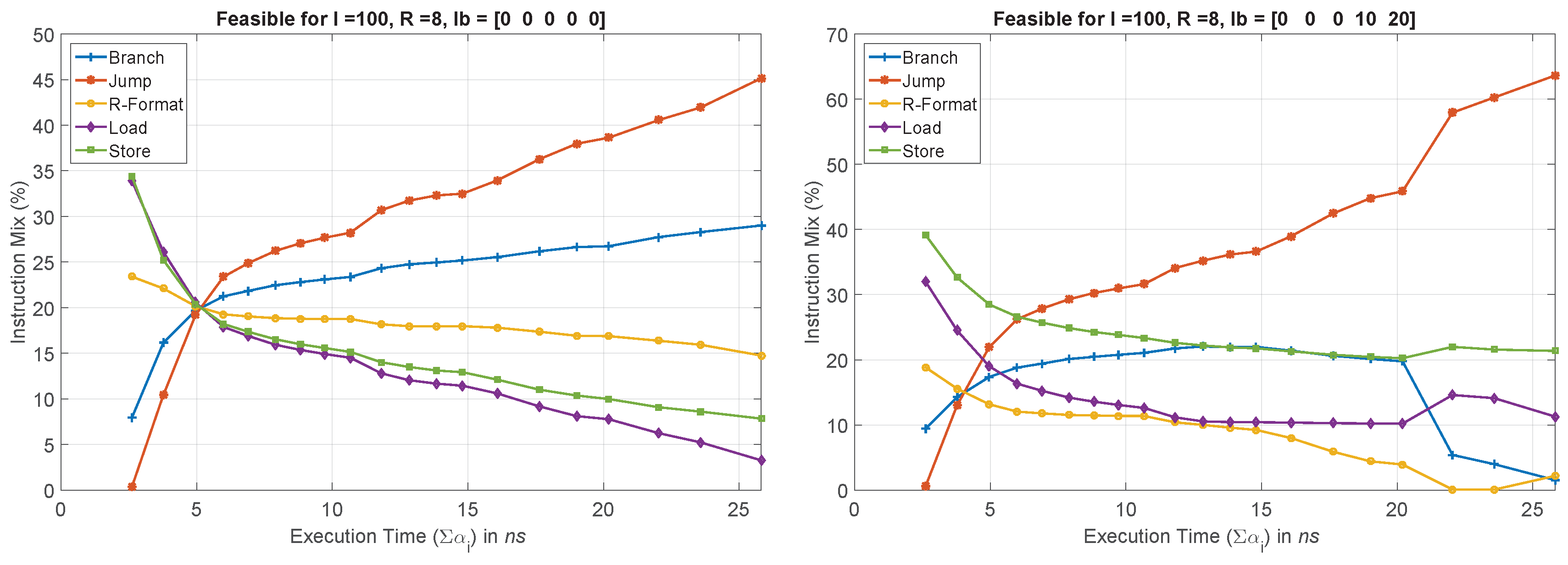
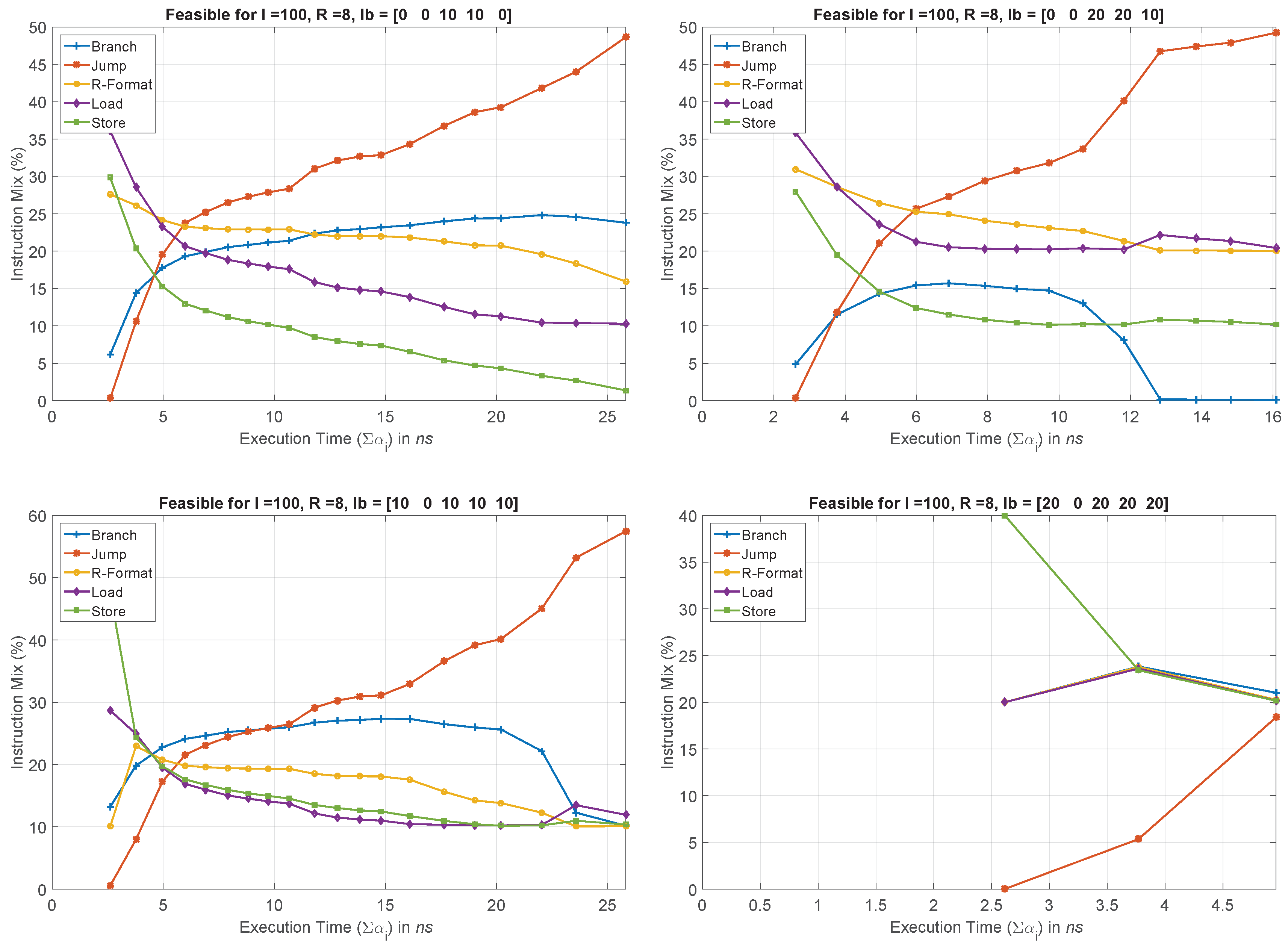
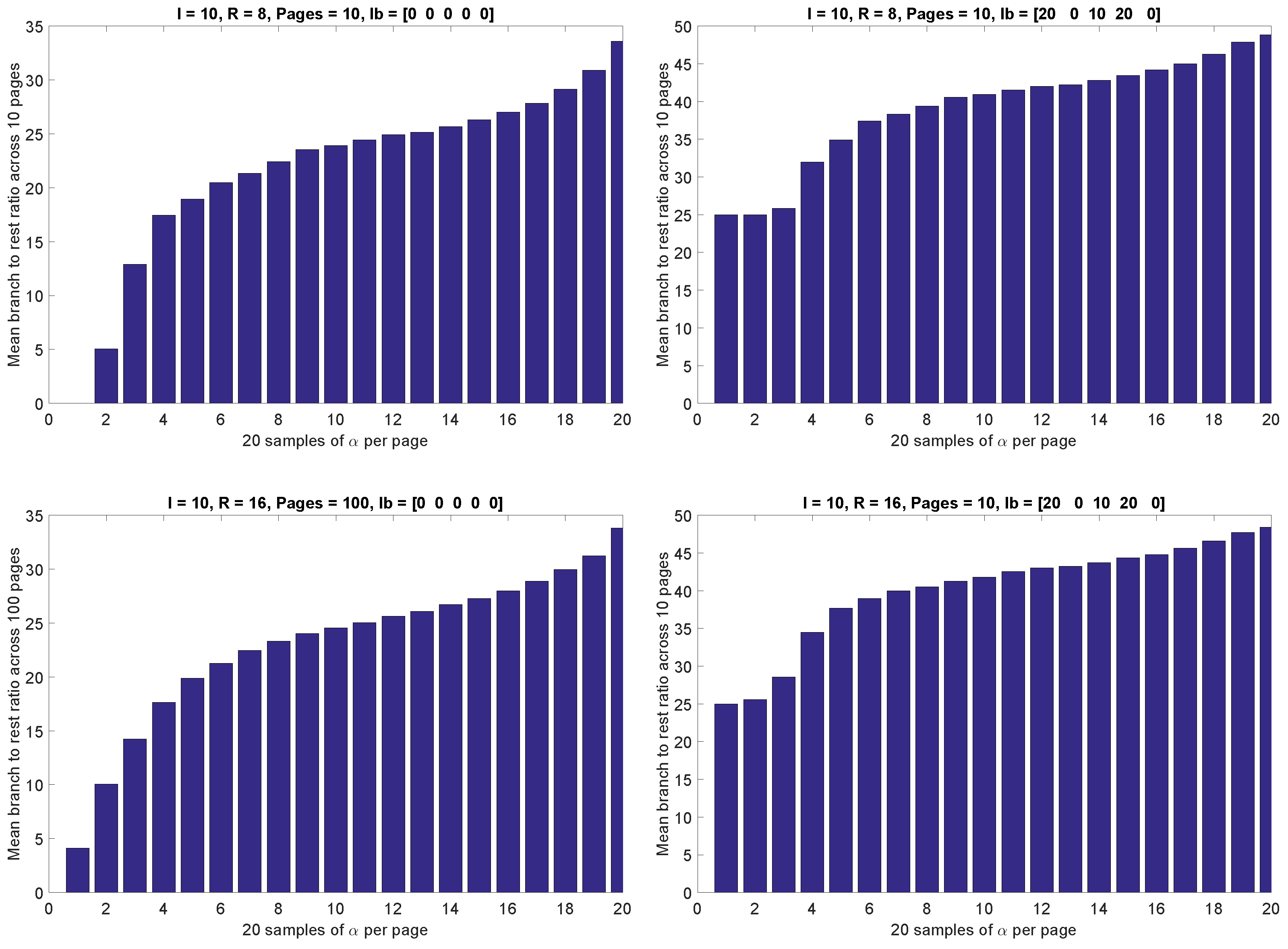
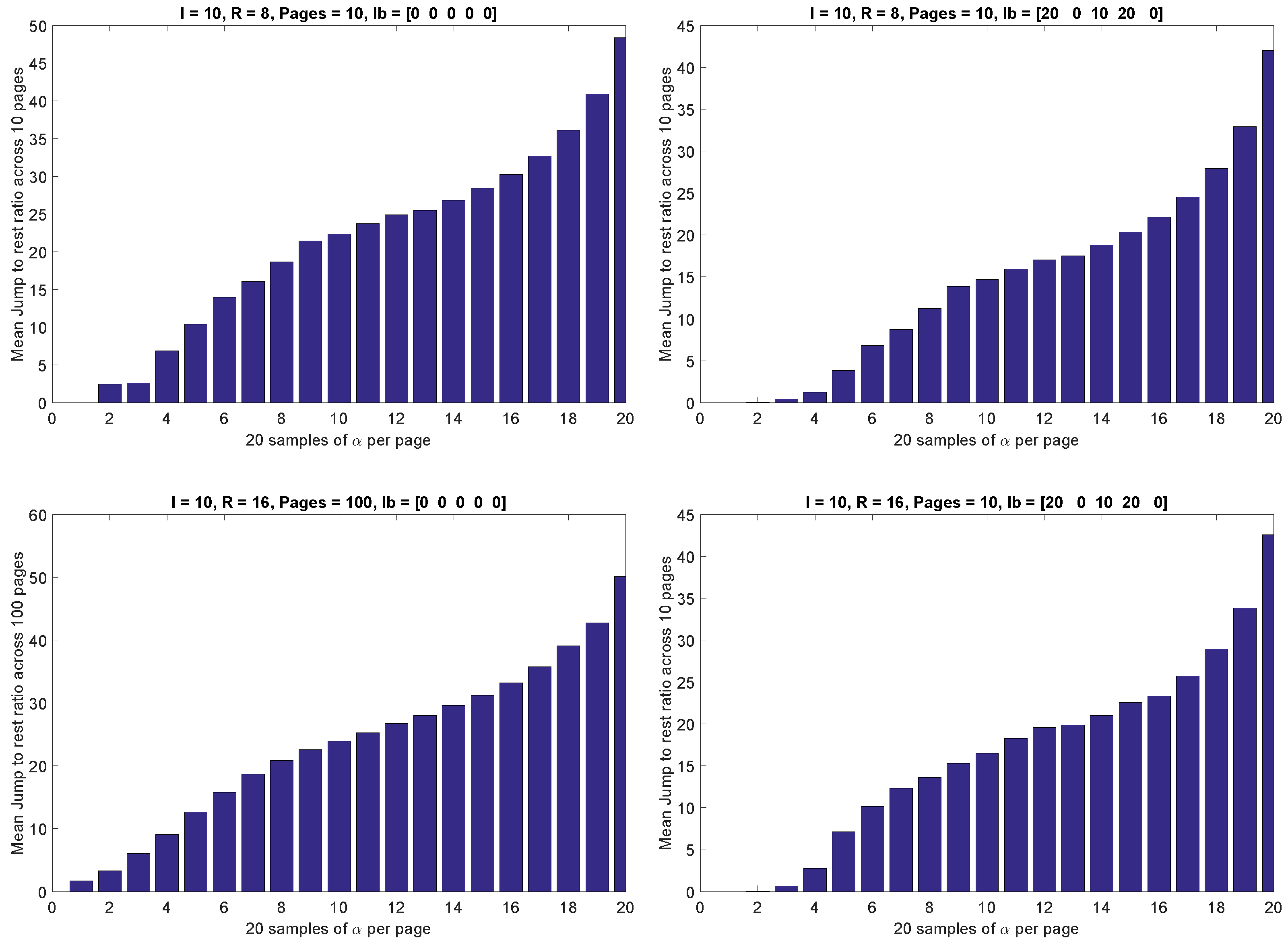
• $lb=\{x_{1\_min},x_{2\_min},x_{3\_min},x_{4\_min},x_{5\_min}\}$— representing lb on each type of instructions, $x_i$, in percentage. Since we already know that jump is the shortest instruction, and will matter the most in yielding feasible solutions to the optimization problems, we do not constrain its lb, and rather treat it as an output. Therefore, $x_{2\_min}=0$. Whereas, we iteratively vary the rest between $\{0,10,20\}$, resulting in $3^4(=81)$ assembly language codes with different instruction mix.

To have acceptable confidence in our results, we had to exploit a larger sample space; we, therefore, randomly generated 1000 values for each ${\alpha }_i$, resulting in a total of $(1000\times codes)=(1000\times 81)$ permutations per assembly language code length per architecture. The results given and discussed below are average values of these total $81,000\times 4=324,000$ iterations for each architecture.

5.2. Simulation Results

Some simulation results for an 8-bit architecture with hundred instructions in the assembly language code, and varying lb are summarized in Figure 4. Each figure in the table plots instruction mix against execution time for a different lb. Please note that advancement in technology will lead to smaller execution times, therefore, x-axis on each plot may represent newer to older processors (from left to right). Before commenting on each result, recall that the optimizer is supposed to find the number of shorter (jump, branch) instructions in a given code such that SCP performs better than the PiP.

In the case of unconstrained lb, i.e., when $lb=[00000]$, observe how conveniently the optimizer is able to find the feasible solutions. Especially at smaller execution times, possible solutions exist without any significant contribution by the shorter instructions. At greater execution times (>20 ns), however, much accumulated contribution (>50%) is needed by the shorter instructions for possible feasible solutions. With increasing lb on $x_3$, $x_4$, and $x_5$, observe how the number of feasible solutions continues to decrease. For example, consider the case when $lb=[00202010]$, i.e., when $x_3$, $x_4$, and $x_5$ together constitute more than half instructions in the given code, the optimizer fails to find feasible solutions beyond execution time 16 ns. Furthermore, the obtained feasible solutions comprise larger percentage of jump instructions. By continuously increasing lb, one may easily observe that the number of feasible solutions continue to drop down. For example, when $lb=[200202020]$, there exists no feasible solution beyond execution time 5 ns. These results are interpreted as follows: for $\sum {\alpha }_i>$ 20 ns, i.e., relatively older processors, an assembly language code, in which jump and branch accumulate for fewer than 50% instructions, suits the PiP more than the SCP. On the other hand, in the case of recent technology nodes with $\sum {\alpha }_i\le$ 5 ns, the codes with merely 20% contribution by the shorter instructions will suit the SCP more than the PiP.

To observe how should the number of branch instructions in a code vary to yield feasible results against increasing execution times, we have plotted the ratio between branch ($x_1)$ and rest of the instructions ($x_3$, $x_4$, and $x_5$), as shown in Figure 5. These results were also generated for the same number of iterations as before, and then their average was computed. For ease of understanding, we have just plotted them for a few specific cases. The trend, however, remains the same for all iterations, as depicted. While the vertical axis, here, corresponds to the obtained ratio between branch and other instructions, the horizontal axis shows the size of each page (we randomly selected 20 samples of ${\alpha }_i$ per page, and the number of pages was 1000). The $\alpha$ samples were initially sorted is ascending order, i.e., the last sample leads to highest execution time (oldest processor in other words). It may be conveniently observed that with increasing execution times, the number of Branch instructions must continue to increase with respect to rest of the instructions, except Jump.

Similarly, Figure 6 presents the case of ratio of Jump to rest of the instructions. Being the shortest instruction in the ISA, the Jump requires its contribution in the given code to be significantly higher than the rest. Once again the trend suggests that for larger execution times, contribution of the shorter instruction, Jump in this case, should be enormous − mostly $\ge 50\%$.

It is important to note in these results that reduction in feature sizes and voltage swings—leading to faster circuits, and therefore, processors—is giving SCP an opportunity to outperform the more modern PiP in average assembly language programs. Therefore, the modern processing platforms are recommended to offer more flexibility, to be able to switch between multiple architectures and design styles, say by means of dynamic partial reconfiguration.

5.3. Sample Codes and Mapping

The following three assembly language codes have been adopted (as they were) from two textbooks: one on MIPS32 and the other on 8051 microprocessors. The purpose of presenting them here is to map each of them to one of the two design paradigms we have discussed, SCP and PiP, with respect to technology, i.e., execution times. Please note that the first two are high-level descriptions, whose assembly codes may be found in the reference book, or with the Supplementary Material.

Code 1: Factorial [2]

$intfact(intn)\{$

$if(n<1)return(1);$

$elsereturn(n\times fact(n-1));\}$

Code 2: Swap & sort [2]

$voidsort(intv[],intn)\{$

$inti,j;$

$for(i=0;i<n;i+=1)\{$

$for(j=i-1;j\ge 0\&\&v[j]>v[j+1];j+=1)\{$

$swap(v,j);\}\}\}$

$voidswap(intv[],intk)\{$

$inttemp;$

$temp=v[k];$

$v[k]=v[k+1];$

$v[k+1]=temp;\}$

Code 3: A 10 kHz square wave using 8051 timers [41]

ORG 8100H
MOV TMOD, #02H	;8-bit auto-reload mode
MOV TH0, #-50	;-50 reload value in TH0
SETB TR0	;start timer
LOOP: JNB TF0 LOOP	;wait for overflow
CLR TF0	;clear timer overflow flag
CPL P1.0	;toggle port bit
SJMP LOOP	;repeat
END

It may be seen in the above codes that use of jumps and branches is increased in scenarios where some operations are to be performed repeatedly, i.e., in loops. In Code 2, the total number of iterations is determined based on n, and the complexity is determined as $\frac{n(n-1)}{2}$ in an average case. In Code 3, the delays are implemented to generate a square wave with 50 percent duty cycle and a period of 100 microseconds. More than 90 percent of the time, processor will be busy in processing jumps and branches. Based on this knowledge, the following code-to-processor mapping, i.e., suitability, may be concluded.

The approximate contribution by Jump and Branch instructions in each of the three codes is $30\%$, $20\%$, and $90\%$ respectively. For these statistics, the proposed framework suggests that Code 1 will map much better on the SCP than the PiP only if execution time, i.e., $\sum {\alpha }_i<$ 5 ns. This may be observed in the top four plots in Figure 4. Similarly, if $\sum {\alpha }_i<$ 3.5 ns, SCP will execute Code 2 better than the PiP. This may be observed in the plot corresponding to $lb=[00202010]$. Finally, for Code 3, SCP will conveniently outperform the PiP for $\sum {\alpha }_i\le$ 45 ns. Please note that these sample codes were chosen because of the fact that they provide a diverse contribution by the instructions favoring the SCP. This has given us significant confidence in the obtained results.

6. Conclusions

The mathematical models that we have developed have suggested that there may be situations, specifically assembly language codes, in which simpler processors may perform better than the more advanced pipelined processors. For a system to yield optimal performance in every situation—post fabrication—it should be possible to switch between the simpler and advanced variants, whichever more suitable, during compile time. To do so, however, one should be able to analyze the given code, and determine which variant it suits more. For this purpose, (1) we have presented performance models for three types of processors, (2) proposed a framework based on a symmetry-targeted non-linear optimization method for code classification, and (3) advocated on using dynamic partial reconfiguration to keep the area and power overhead of the system to minimum, besides making it flexible for swift switching. Our analysis is thorough, and it leads to the conclusion that for recent technology nodes, in the submicron era, it is even more convenient for simpler processors to outperform the pipelined processors. Therefore, the modern systems should flexibly adapt to the given situation by means of dynamic partial reconfiguration.

As a prospective step, following this theoretical framework, we aim to (1) design the three types of processors on an FPGA, supporting dynamic partial reconfiguration, (2) execute multiple benchmark codes available in the literature, (3) estimate the performance of each type, and (4) carrying out a detailed quantitative comparison between them. This will help us practically validate our mathematical models, and will give us confidence in our claim.

References

1. Patterson, D.A.; Sequin, C.H. RISC I: A Reduced Instruction Set VLSI Computer. In Proceedings of the 8th Annual Symposium on Computer Architecture ISCA ’81, Minneapolis, MN, USA, 12–14 May 1981; IEEE Computer Society Press: Los Alamitos, CA, USA, 1981; pp. 443–457. [Google Scholar]
2. Patterson, D.A.; Hennessy, J.L. Computer Organization and Design MIPS Edition: The Hardware/Software Interface; Newnes: Bathurst, Australia, 2013. [Google Scholar]
3. Kumar, R.; Pawar, L.; Aggarwal, A. Smartphones hardware Architectures and Their Issues. Int. J. Eng. Res. Appl. 2014, 4, 81–83. [Google Scholar]
4. Fu, H.; Liao, J.; Yang, J.; Wang, L.; Song, Z.; Huang, X.; Yang, C.; Xue, W.; Liu, F.; Qiao, F.; et al. The Sunway TaihuLight supercomputer: system and applications. Sci. China Inf. Sci. 2016, 59, 072001. [Google Scholar] [CrossRef]
5. David, A.P.; John, L.H. Computer Organization and Design: The Hardware/Software Interface; Morgan Kaufmann Publishers: San mateo, CA, USA, 2005; Volume 1, p. 998. [Google Scholar]
6. Obaidat, M.; Abu-Saymeh, D.S. Performance of RISC-based multiprocessors. Comput. Electr. Eng. 1993, 19, 185–192. [Google Scholar] [CrossRef]
7. Shen, J.P.; Lipasti, M.H. Modern Processor Design: Fundamentals of Superscalar Processors; Waveland Press: Long Grove, IL, USA, 2013. [Google Scholar]
8. Vargas, V.; Ramos, P.; Méhaut, J.F.; Velazco, R. NMR-MPar: A fault-tolerance approach for multi-core and many-core processors. Appl. Sci. 2018, 8, 465. [Google Scholar] [CrossRef]
9. Wang, S.H.; Peng, W.H.; He, Y.; Lin, G.Y.; Lin, C.Y.; Chang, S.C.; Wang, C.N.; Chiang, T. A software-hardware co-implementation of MPEG-4 advanced video coding (AVC) decoder with block level pipelining. J. VLSI Signal Process. Syst. Signal Image Video Technol. 2005, 41, 93–110. [Google Scholar] [CrossRef]
10. Khan, S.; Rashid, M.; Javaid, F. A high performance processor architecture for multimedia applications. Comput. Electr. Eng. 2018, 66, 14–29. [Google Scholar] [CrossRef]
11. Liu, Q.; Xu, Z.; Yuan, Y. High throughput and secure advanced encryption standard on field programmable gate array with fine pipelining and enhanced key expansion. IET Comput. Digit. Tech. 2015, 9, 175–184. [Google Scholar] [CrossRef]
12. Mukhtar, N.; Mehrabi, M.; Kong, Y.; Anjum, A. Machine-Learning-Based Side-Channel Evaluation of Elliptic-Curve Cryptographic FPGA Processor. Appl. Sci. 2019, 9, 64. [Google Scholar] [CrossRef]
13. Tummala, R.; Nedumthakady, N.; Ravichandran, S.; DeProspo, B.; Sundaram, V. Heterogeneous and homogeneous package integration technologies at device and system levels. In Proceedings of the Pan Pacific Microelectronics Symposium (Pan Pacific), Waimea, HI, USA, 5–8 February 2018; pp. 1–5. [Google Scholar]
14. Hussein, F.; Daoud, L.; Rafla, N. HexCell: a Hexagonal Cell for Evolvable Systolic Arrays on FPGAs. In Proceedings of the 2018 ACM/SIGDA International Symposium on Field-Programmable Gate Arrays, Monterey, CA, USA, 25–27 February 2018; p. 293. [Google Scholar]
15. Skvortsov, V.V.; Zvyagina, M.I.; Skitev, A.A. Sharing resources in heterogeneous multitasking computer systems based on FPGA with the use of partial reconfiguration. In Proceedings of the 2018 IEEE Conference of Russian Young Researchers in Electrical and Electronic Engineering (EIConRus), Moscow, Russia, 29 January–1 February 2018; pp. 370–373. [Google Scholar]
16. Alfian, G.; Syafrudin, M.; Yoon, B.; Rhee, J. False Positive RFID Detection Using Classification Models. Appl. Sci. 2019, 9, 1154. [Google Scholar] [CrossRef]
17. Gu, X.; Fang, L.; Liu, P.; Hu, Q. Multiple Chip Multiprocessor Cache Coherence Operation Method and Multiple Chip Multiprocessor. U.S. Patent 16/138,824, 24 January 2019. [Google Scholar]
18. Pezzarossa, L.; Kristensen, A.T.; Schoeberl, M.; Sparsø, J. Can Real-Time Systems Benefit from Dynamic Partial Reconfiguration? In Proceedings of the Nordic Circuits and Systems Conference (NORCAS): NORCHIP and International Symposium of System-on-Chip (SoC), Linköping, Sweden, 23–25 October 2017.
19. Pezzarossa, L.; Schoeberl, M.; Sparsø, J. Reconfiguration in FPGA-based multi-core platforms for hard real-time applications. In Proceedings of the 11th International Symposium on Reconfigurable Communication-centric Systems-on-Chip (ReCoSoC), Tallinn, Estonia, 27–29 June 2016; pp. 1–8. [Google Scholar]
20. Hassan, A.; Mostafa, H.; Fahmy, H.A.; Ismail, Y. Exploiting the Dynamic Partial Reconfiguration on NoC-Based FPGA. In Proceedings of the 2017 New Generation of Exploiting the Dynamic Partial Reconfiguration on NoC-Based FPGA, Genoa, Italy, 6–9 September 2017; pp. 277–280. [Google Scholar]
21. Becher, A.; Bauer, F.; Ziener, D.; Teich, J. Energy-aware SQL query acceleration through FPGA-based dynamic partial reconfiguration. In Proceedings of the 24th International Conference on IEEE Field Programmable Logic and Applications (FPL), Munich, Germany, 2–4 September 2014; pp. 1–8. [Google Scholar]
22. Johnson, A.P.; Liu, J.; Millard, A.G.; Karim, S.; Tyrrell, A.M.; Harkin, J.; Timmis, J.; McDaid, L.J.; Halliday, D.M. Homeostatic Fault Tolerance in Spiking Neural Networks: A Dynamic Hardware Perspective. IEEE Trans. Circuits Syst. I Regul. Pap. 2018, 65, 687–699. [Google Scholar] [CrossRef]
23. Birk, Y.; Fiksman, E. Dynamic reconfiguration architectures for multi-context FPGAs. Comput. Electr. Eng. 2009, 35, 878–903. [Google Scholar] [CrossRef]
24. Emami, S.; Sedighi, M. An optimized reconfigurable architecture for hardware implementation of decimal arithmetic. Comput. Electr. Eng. 2017, 63, 18–29. [Google Scholar] [CrossRef]
25. Aagaard, M.; Leeser, M. Reasoning about pipelines with structural hazards. In Theorem Provers in Circuit Design; Springer: Berlin, Germany, 1995; pp. 13–32. [Google Scholar] [Green Version]
26. Alghunaim, S.A.; Sayed, A.H. Distributed coupled multi-agent stochastic optimization. IEEE Trans. Autom. Control 2019. [Google Scholar] [CrossRef]
27. Abed-alguni, B.H. Island-based Cuckoo Search with Highly Disruptive Polynomial Mutation. Int. J. Artif. Intell. 2019, 17, 57–82. [Google Scholar]
28. Shams, M.; Rashedi, E.; Dashti, S.M.; Hakimi, A. Ideal gas optimization algorithm. Int. J. Artif. Intell. 2017, 15, 116–130. [Google Scholar]
29. Soares, A.; Râbelo, R.; Delbem, A. Optimization based on phylogram analysis. Expert Syst. Appl. 2017, 78, 32–50. [Google Scholar] [CrossRef]
30. Precup, R.E.; David, R.C. Nature-Inspired Optimization Algorithms for Fuzzy Controlled Servo Systems; Butterworth-Heinemann: Oxford, UK, 2019. [Google Scholar]
31. Esbensen, H. Computing near-optimal solutions to the Steiner problem in a graph using a genetic algorithm. Networks 1995, 26, 173–185. [Google Scholar] [CrossRef]
32. Oulghelou, M.; Allery, C. Hyper bi-calibrated interpolation on the Grassmann manifold for near real time flow control using genetic algorithm. arXiv, 2019; arXiv:1903.03611. [Google Scholar]
33. Fushchich, W.I.; Shtelen, W.; Serov, N. Symmetry Analysis and Exact Solutions of Equations of Nonlinear Mathematical Physics; Springer: Berlin, Germany, 1997. [Google Scholar]
34. Zoutendijk, G. Methods of Feasible Directions: A Study in Linear and Non-Linear Programming; Elsevier: Amsterdam, The Netherlands, 1960. [Google Scholar]
35. Bazaraa, M.S.; Sherali, H.D.; Shetty, C.M. Nonlinear Programming: Theory andAlgorithms; John Wiley & Sons: Hoboken, NJ, USA, 2013. [Google Scholar]
36. Zhang, S.; Huang, J.; Yang, J. Raising Power Loss Equalizing Degree of Coil Array by Convex Quadratic Optimization Commutation for Magnetic Levitation Planar Motors. Appl. Sci. 2019, 9, 79. [Google Scholar] [CrossRef]
37. Shachar, N.; Mitelpunkt, A.; Kozlovski, T.; Galili, T.; Frostig, T.; Brill, B.; Marcus-Kalish, M.; Benjamini, Y. The importance of nonlinear transformations use in medical data analysis. JMIR Med. Inform. 2018, 6, e27. [Google Scholar] [CrossRef]
38. Westerlund, T.; Lundell, A.; Westerlund, J. On convex relaxations in nonconvex optimization. Chem. Eng. Trans. 2011, 24, 331–336. [Google Scholar]
39. Castro, P.M. Tightening piecewise McCormick relaxations for bilinear problems. Comput. Chem. Eng. 2015, 72, 300–311. [Google Scholar] [CrossRef] [Green Version]
40. Hinder, O.; Ye, Y. A one-phase interior point method for nonconvex optimization. arXiv, 2018; arXiv:1801.03072. [Google Scholar]
41. MacKenzie, I.S.; Phan, R.C.W. The 8051 Microcontroller; Prentice Hall: Upper Saddle River, NJ, USA, 1999; Volume 3. [Google Scholar]
Figure 1. Timing in each processor variant.
Symmetry 11 00938 g001
Figure 2. McCormick Envelopes: under and over estimators (reprinted).
Symmetry 11 00938 g002
Figure 3. Proposed Methodology.
Symmetry 11 00938 g003
Figure 4. Instruction mix for feasible solutions with varying lower bounds (lb).
Symmetry 11 00938 g004aSymmetry 11 00938 g004b
Figure 5. Ratio of branch instruction to rest for feasible solutions.
Symmetry 11 00938 g005
Figure 6. Ratio of jump instruction to rest for feasible solutions.
Symmetry 11 00938 g006