Radial and Bilateral Fluctuating Asymmetry of Iris pumila Flowers as Indicators of Environmental Stress

 ,
,
Abstract
:1. Introduction
2. Materials and Methods
2.1. Species Description
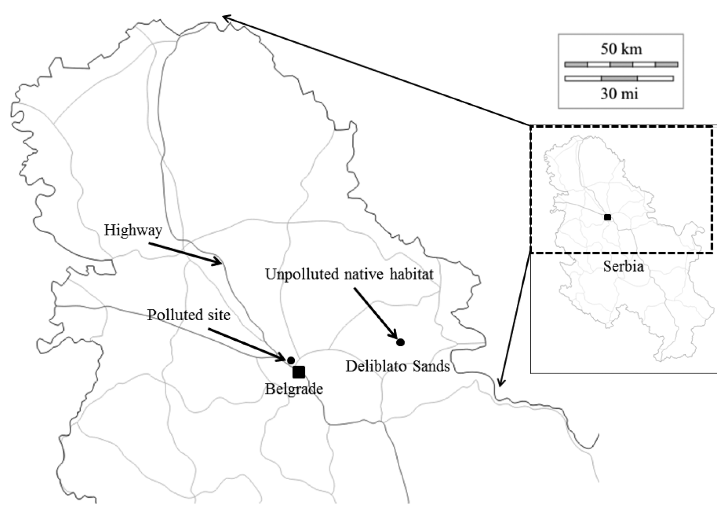
2.2. Study Sites
2.3. Sampling Design
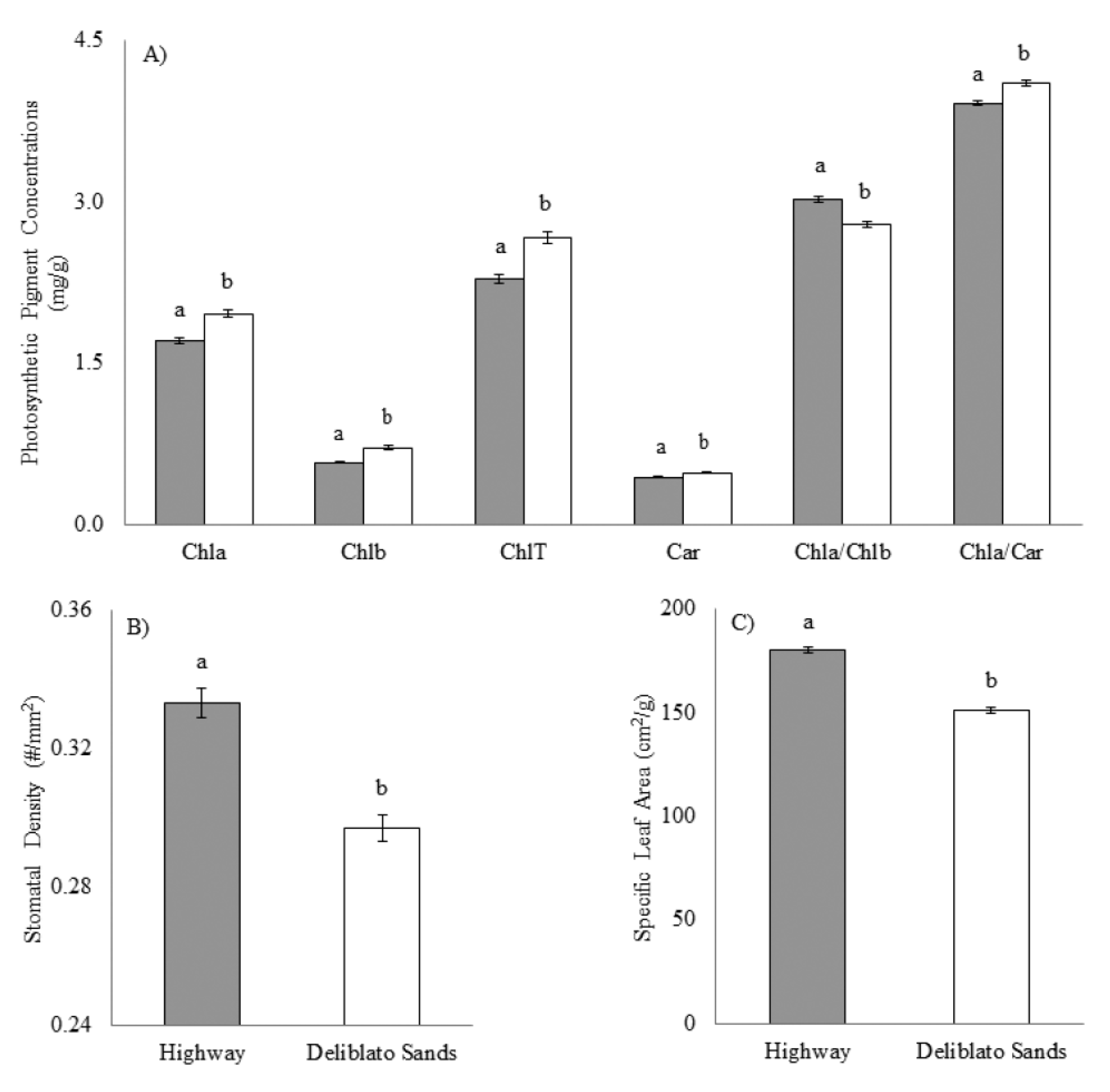
2.3.1. Photosynthetic Pigment Concentrations, Stomatal Density, and Specific Leaf Area
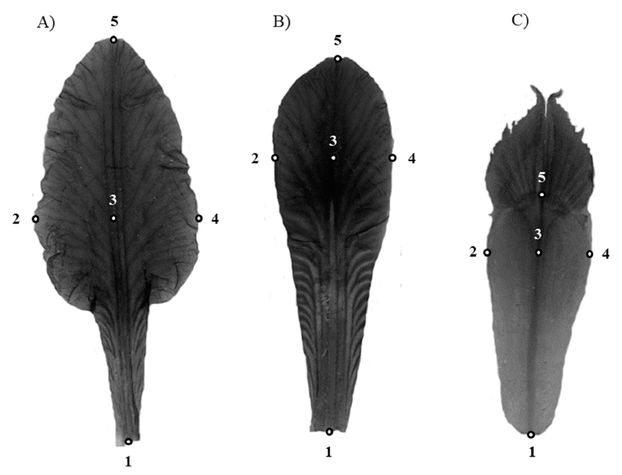
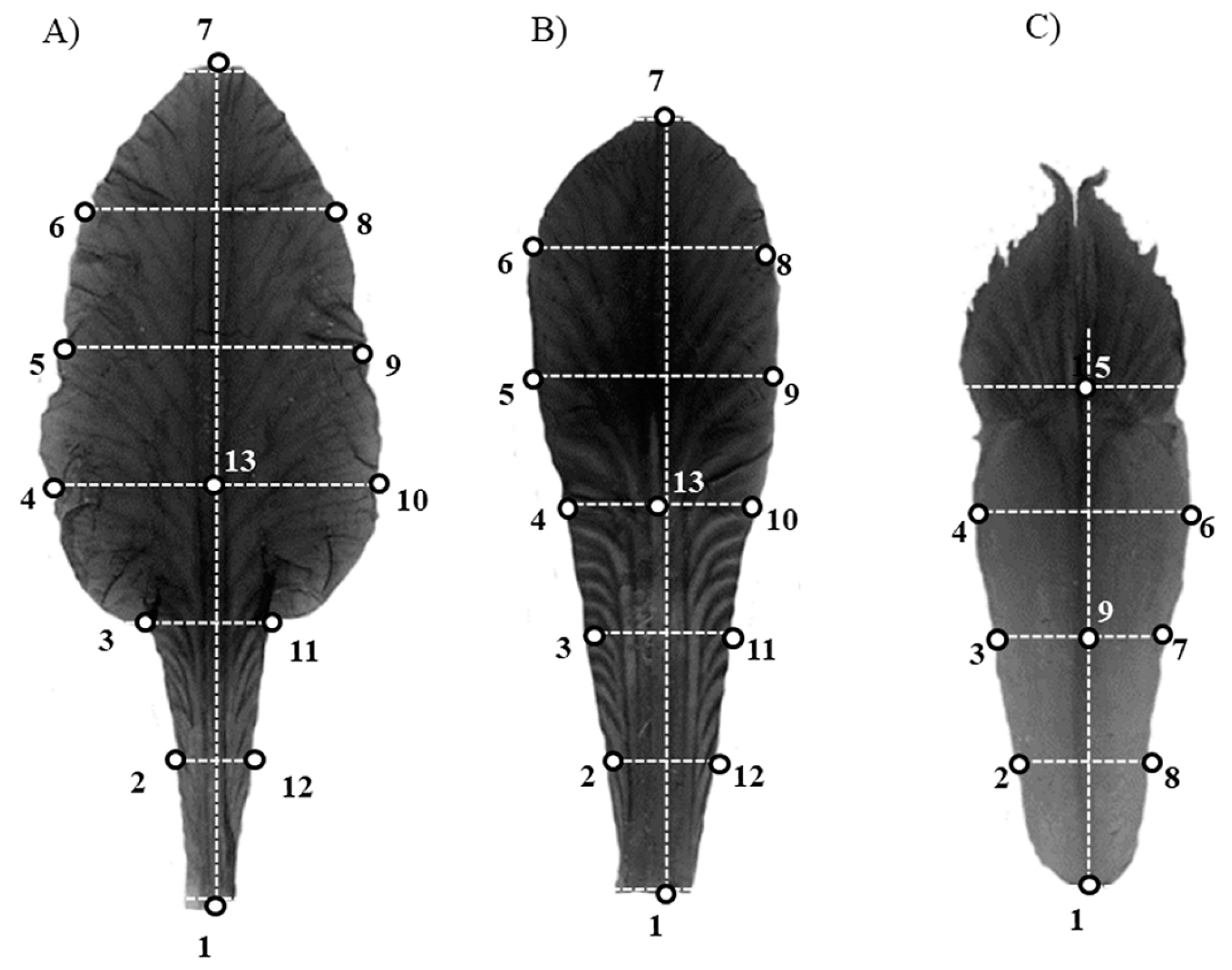
2.3.2. Radial and Bilateral Fluctuating Asymmetry
Linear Morphometrics
Geometric Morphometrics
2.4. Statistical Analyses
2.4.1. Photosynthetic Pigment Concentrations, Stomatal Density, and Specific Leaf Area
2.4.2. Radial and Bilateral Fluctuating Asymmetry
Linear Morphometrics
Geometric Morphometrics
3. Results
3.1. Photosynthetic Pigment Concentrations, Stomatal Density, and Specific Leaf Area
3.2. Radial and Bilateral Fluctuating Asymmetry
3.2.1. Linear Morphometrics
3.2.2. Geometric Morphometrics
4. Discussion
5. Conclusions
- The chosen site was proven stressful and, therefore, appropriate for testing the suitability of various flower asymmetry indices, as demonstrated by lower levels of photosynthetic pigment concentrations and higher stomatal density and specific leaf area, in transplanted plants.
- All but one of the analyzed asymmetry indices failed to detect a significant effect of a heavily polluted environment, with a demonstrated stressful effect on Iris pumila plants.
- Iris pumila flower asymmetry is not suitable for biomonitoring purposes.
Author Contributions
Funding
Acknowledgments
Conflicts of Interest
References
- Møller, A.P.; Shykoff, J.A. Morphological developmental stability in plants: Patterns and causes. Int. J. Plant Sci. 1999, 160, S135–S146. [Google Scholar] [CrossRef] [PubMed]
- Palmer, A.R.; Strobeck, C. Fluctuating asymmetry analyses revisited. In Developmental Instability: Causes and Consequences; Polak, M., Ed.; Oxford University Press: Oxford, UK, 2003; pp. 279–319. [Google Scholar]
- Clarke, G.M. The genetic basis of developmental stability. V. Inter- and intra-individual character variation. Heredity 1998, 80, 562–567. [Google Scholar] [CrossRef]
- Van Dongen, S. How repeatable is the estimation of developmental stability by fluctuating asymmetry? Proc. R. Soc. B Biol. Sci. 1998, 265, 1423–1427. [Google Scholar] [CrossRef]
- Graham, J.H.; Raz, S.; Hel-Or, H.; Nevo, E. Fluctuating asymmetry: Methods, theory, and applications. Symmetry 2010, 2, 466–540. [Google Scholar] [CrossRef]
- Palmer, A.R. Fluctuating asymmetry analyses: A primer. In Developmental Instability: Its Origins and Evolutionary Implications; Markow, T.A., Ed.; Kluwer: Dordrecht, The Netherlands, 1994; pp. 335–364. [Google Scholar]
- Angold, P.G. The impact of a road upon adjacent heathland vegetation: Effects on plant species composition. J. Appl. Ecol. 1997, 34, 409–417. [Google Scholar] [CrossRef]
- Cottingham, K.L.; Carpenter, S.R. Population, community, and ecosystem variates as ecological indicators: Phytoplankton responses to whole-lake enrichment. Ecol. Appl. 1998, 8, 508–530. [Google Scholar] [CrossRef]
- Komac, B.; Alados, C.L. Fluctuating asymmetry and Echinospartum horridum fitness components. Ecol. Indic. 2012, 18, 252–258. [Google Scholar] [CrossRef]
- Alados, C.L.; Navarro, T.; Escós, J.; Cabezudo, B.; Emlen, J.M. Translational and fluctuating asymmetry as tools to detect stress in stress-adapted and nonadapted plants. Int. J. Plant Sci. 2001, 162, 607–616. [Google Scholar] [CrossRef]
- Balasooriya, B.L.W.K.; Samson, R.; Mbikwa, F.; Vitharana, U.W.A.; Boeckx, P.; Van Meirvenne, M. Biomonitoring of urban habitat quality by anatomical and chemical leaf characteristics. Environ. Exp. Bot. 2009, 65, 386–394. [Google Scholar] [CrossRef]
- Cañas, M.S.; Carreras, H.A.; Orellana, L.; Pignata, M.L. Correlation between environmental conditions and foliar chemical parameters in Ligustrum lucidum Ait. exposed to urban air pollutants. J. Environ. Manag. 1997, 49, 167–181. [Google Scholar]
- Carreras, H.A.; Cañas, M.S.; Pignata, M.L. Differences in responses to urban air pollutants by Ligustrum lucidum Ait. and Ligustrum lucidum Ait. f. tricolor (Rehd.) Rehd. Environ. Pollut. 1996, 93, 211–218. [Google Scholar] [CrossRef]
- Markert, B. Definitions and principles for bioindication and biomonitoring of trace metals in the environment. J. Trace Elem. Med. Biol. 2007, 21, 77–82. [Google Scholar] [CrossRef] [PubMed]
- Graham, J.H.; Duda, J.J.; Brown, M.L.; Kitchen, S.; Emlen, J.M.; Malol, J.; Bankstahl, E.; Krzysik, A.J.; Balbach, H.; Freeman, D.C. The effects of drought and disturbance on the growth and developmental instability of loblolly pine (Pinus taeda L.). Ecol. Indic. 2012, 20, 143–150. [Google Scholar] [CrossRef]
- Raz, S.; Graham, J.H.; Hel-Or, H.; Pavlíček, T.; Nevo, E. Developmental instability of vascular plants in contrasting microclimates at ‘Evolution Canyon’. Biol. J. Linn. Soc. 2011, 102, 786–797. [Google Scholar] [CrossRef]
- Barišić Klisarić, N.; Miljković, D.; Avramov, S.; Živković, U.; Tarasjev, A. Fluctuating asymmetry in Robinia pseudoacacia leaves—Possible in situ biomarker? Environ. Sci. Pollut. Res. 2014, 21, 12928–12940. [Google Scholar] [CrossRef] [PubMed]
- Venâncio, H.; Alves-Silva, E.; Santos, J.C. Leaf phenotypic variation and developmental instability in relation to different light regimes. Acta Bot. Bras. 2016, 30, 296–303. [Google Scholar] [CrossRef] [Green Version]
- Kozlov, M.V.; Wilsey, B.J.; Koricheva, J.; Haukioja, E. Fluctuating asymmetry of birch leaves increases under pollution impact. J. Appl. Ecol. 1996, 33, 1489–1495. [Google Scholar] [CrossRef]
- Watson, P.J.; Thornhill, R. Fluctuating asymmetry and sexual selection. Trends Ecol. Evol. 1994, 9, 21–25. [Google Scholar] [CrossRef]
- Citerne, H.; Jabbour, F.; Nadot, S.; Damerval, C. The Evolution of Floral Symmetry. Adv. Bot. Res. 2010, 54, 85–137. [Google Scholar]
- Klingenberg, C.P. Analyzing fluctuating asymmetry with geometric morphometrics: Concepts, methods, and applications. Symmetry 2015, 7, 843–934. [Google Scholar] [CrossRef]
- Endress, P.K. Symmetry in Flowers: Diversity and Evolution. Int. J. Plant Sci. 1999, 160, S3–S23. [Google Scholar] [CrossRef] [PubMed] [Green Version]
- Møller, A.P.; Sorci, G. Insect preference for symmetrical artificial flowers. Oecologia 1998, 114, 37–42. [Google Scholar] [CrossRef] [PubMed]
- Møller, A.P.; Eriksson, M. Pollinator preference for symmetrical flowers and sexual selection in plants. Oikos 1995, 73, 15–22. [Google Scholar] [CrossRef]
- Alados, C.L.; Giner, M.L.; Dehesa, L.; Escos, J.; Barroso, F.G.; Emlen, J.M.; Freeman, D.C. Developmental instability and fitness in Periploca laevigata experiencing grazing disturbance. Int. J. Plant Sci. 2002, 163, 969–978. [Google Scholar] [CrossRef]
- Tucić, B.; Miljković, D. Fluctuating asymmetry of floral organ traits in natural populations of Iris pumila from contrasting light habitats. Plant Species Biol. 2010, 25, 173–184. [Google Scholar] [CrossRef]
- Helsen, P.; Van Dongen, S. Associations between floral asymmetry and individual genetic variability differ among three Prickly Pear (Opuntia echios) populations. Symmetry 2016, 8, 116. [Google Scholar] [CrossRef]
- Tarasjev, A.; Avramov, S.; Miljković, D. Evolutionary biology studies on the Iris pumila clonal plant: Advantages of a good model system, main findings and directions for further research. Arch. Biol. Sci. 2012, 64, 159–174. [Google Scholar] [CrossRef]
- Miljković, D. Developmental stability of Iris pumila flower traits: A common garden experiment. Arch. Biol. Sci. 2012, 64, 123–133. [Google Scholar] [CrossRef]
- Radović, S.; Urosević, A.; Hočevar, K.; Vuleta, A.; Manitasević-Jovanović, S.; Tucić, B. Geometric morphometrics of functionally distinct floral organs in Iris pumila: Analyzing patterns of symmetric and asymmetric shape variations. Arch. Biol. Sci. 2017, 69, 223–231. [Google Scholar] [CrossRef]
- Tarasjev, A. Relationship between phenotypic plasticity and developmental instability in Iris pumila L. Russ. J. Genet. 1995, 31, 1409–1416. [Google Scholar]
- Hogg, I.D.; Eadie, J.M.; Dudley Williams, D.; Turner, D. Evaluating fluctuating asymmetry in a stream-dwelling insect as an indicator of low-level thermal stress: A large-scale field experiment. J. Appl. Ecol. 2001, 38, 1326–1339. [Google Scholar] [CrossRef]
- Gostin, I.N. Air pollution effects on the leaf structure of some Fabaceae species. Not. Bot. Horti Agrobot. Cluj-Napoca 2009, 37, 57–63. [Google Scholar]
- Arellano, P.; Tansey, K.; Balzter, H.; Tellkamp, M.; Martin, R.; Bidel, L. Plant family-specific impacts of petroleum pollution on biodiversity and leaf chlorophyll content in the Amazon rainforest of Ecuador. PLoS ONE 2017, 12, e0169867. [Google Scholar] [CrossRef]
- Pignata, M.L.; Gudifio, G.L.; Cafiasa, M.S.; Orellanab, L. Relationship between foliar chemical parameters measured in Melia azedarach L. and environmental conditions in urban areas. Sci. Total Environ. 1999, 243–244, 85–96. [Google Scholar] [CrossRef]
- Haruna, H.; Aliko, A.A.; Ahmad, F.A.; Abubakar, A.W. Effect of automobile exhaust on some leaf micromorphological characteristics of some members of Verbanaceae, Annonaceae and Euphorbiaceae families. Bayero J. Pure Appl. Sci. 2017, 10, 251–258. [Google Scholar] [CrossRef]
- Shiv, K.; Ila, P. Stomatal analysis in Cassia occidentalis L. in response to automobile pollution along roadsides in Meerut city, India. Int. Res. J. Sci. Eng. 2014, 2, 167–170. [Google Scholar]
- Dineva, S.B. Comparative studies of the leaf morphology and structure of white ash Fraxinus americana L. and London plane tree Platanus acerifolia Willd. growing in polluted area. Dendrobiology 2004, 52, 3–8. [Google Scholar]
- Wuytack, T.; Wuyts, K.; Van Dongen, S.; Baeten, L.; Kardel, F.; Verheyen, K.; Samson, R. The effect of air pollution and other environmental stressors on leaf fluctuating asymmetry and specific leaf area of Salix alba L. Environ. Pollut. 2011, 159, 2405–2411. [Google Scholar] [CrossRef]
- Poorter, H.; Niinemets, Ü.; Poorter, L.; Wright, I.J.; Villar, R. Causes and consequences of variation in leaf mass per area (LMA): A meta-analysis. New Phytol. 2009, 182, 565–588. [Google Scholar] [CrossRef]
- Mitra, J. Karyotype Analysis of Bearded Iris. Bot. Gaz. 1955, 117, 265–293. [Google Scholar] [CrossRef]
- Purger, D.; Csiky, J.; Topić, J. Dwarf iris, Iris pumila L. (Iridaceae), a new species of the Croatian flora. Acta Bot. Croat. 2008, 67, 97–102. [Google Scholar]
- Randolph, L.F. The geographic distribution of European and Eastern Mediterranean species of bearded Iris. In Iris Year Book; British Iris Society: Tunbridge Wells, UK, 1955; pp. 35–46. [Google Scholar]
- Stevanović, V. The Red Data Book of Flora of Serbia 1. Extinct and Extremely Endangered Taxa; Stevanović, V., Tatić, B., Eds.; Ministry of the Environment of the Republic of Serbia, Faculty of Biology, University of Belgrade, Institute for Protection of Nature of the Republic of Serbia: Belgrade, Serbia, 1999. [Google Scholar]
- Stjepanović-Veseličić, L. Vegetation of the Deliblato Sands; Institute for Ecology and Biogeography: Belgrade, Serbia, 1953. [Google Scholar]
- Goldblatt, P.; Manning, J.C. The Iris Family: Natural History and Classification; Timber Press: Portland, OR, USA, 2008; ISBN 0881928976. [Google Scholar]
- Wu, Q.-G.; Cutler, D.F. Taxonomic, evolutionary and ecological implications of the leaf anatomy of rhizomatous Iris species. Bot. J. Linn. Soc. 1985, 90, 253–303. [Google Scholar] [CrossRef]
- Neal, P.R.; Dafni, A.; Giurfa, M. Floral symmetry and its role in plant-pollinator systems: Terminology, distribution, and hypotheses. Annu. Rev. Ecol. Syst. 1998, 29, 345–373. [Google Scholar] [CrossRef]
- UNESCO. WHC Tentative List; UNESCO World Heritage Centre: Paris, France, 2002. [Google Scholar]
- The Government of the Republic of Serbia. Decree on Criteria for State Road Categorization; Official Gazette of the Republic of Serbia: Belgrade, Serbia, 2013.
- Jayaratne, E.R.; Wang, L.; Heuff, D.; Morawska, L.; Ferreira, L. Increase in particle number emissions from motor vehicles due to interruption of steady traffic flow. Transp. Res. Part D Transp. Environ. 2009, 14, 521–526. [Google Scholar] [CrossRef] [Green Version]
- Tarasjev, A. Flowering phenology in natural populations of Iris pumila. Ecography 1997, 20, 48–54. [Google Scholar] [CrossRef]
- Tarasjev, A.; Barisić Klisarić, N.; Stojković, B.; Avramov, S. Phenotypic plasticity and between population differentiation in Iris pumila transplants between native open and anthropogenic shade habitats. Russ. J. Genet. 2009, 45, 944–952. [Google Scholar] [CrossRef]
- Tarasjev, A.; Tucić, B. Morphological differentiation of Iris pumila populations in Deliblato sands. In Proceedings of the Deliblato Sands Conference, Belgrade, Serbia, January 1994; Volume 6, pp. 289–297. [Google Scholar]
- Hiscox, J.D.; Israelstam, G.F. A method for the extraction of chlorophyll from leaf tissue without maceration. Can. J. Bot. 1979, 57, 1332–1334. [Google Scholar] [CrossRef]
- Minocha, R.; Martinez, G.; Lyons, B.; Long, S. Development of a standardized methodology for quantifying total chlorophyll and carotenoids from foliage of hardwood and conifer tree species. Can. J. Res. 2009, 39, 849–861. [Google Scholar] [CrossRef]
- Pazourek, J. The effect of light intensity on stomatal frequency in leaves of Iris hollandica hort., var. wedgwood. Biol. Plant. 1970, 12, 208–215. [Google Scholar] [CrossRef]
- Wilson, P.J.; Thompson, K.; Hodgson, J.G. Specific leaf area and leaf dry matter content as alternative predictors of plant strategies. New Phytol. 1999, 143, 155–162. [Google Scholar] [CrossRef]
- Sheets, H.D.; Zelditch, M. TMorphGen6. 2003. Available online: http://www3.canisiuse.du/~sheets/ morphsofthtml (accessed on 15 December 2013).
- Rohlf, F.J. TpsDIG 2.16. 2010. Available online: http://life.bio.sunysb.edu/morph/soft- dataacq.html (accessed on 15 December 2013).
- Sheets, H.D. Imp, Integrated Morphometric Package. 2000. Available online: http://www.canisius.edu/~sheets/morphsoft.html (accessed on 15 December 2003).
- Klingenberg, C.P. MorphoJ: An integrated software package for geometric morphometrics. Mol. Ecol. Resour. 2011, 11, 353–357. [Google Scholar] [CrossRef] [PubMed]
- Klingenberg, C.P.; Barluenga, M.; Meyer, A. Shape analysis of symmetric structures: Quantifying variation among individuals and asymmetry. Evolution 2002, 56, 1909–1920. [Google Scholar] [CrossRef] [PubMed]
- SAS Institute SAS 9.1.3 2011. Statistical Analysis System Institute, Inc. 2011. The SAS System for Windows (release 9.3.). Cary, North Carolina, USA. Available online: http://support.sas.com/software/93/ (accessed on 17 June 2019).
- Scheffe, H. A Method for judging all contrasts in the analysis of variance. Biometrika 1953, 40, 87–104. [Google Scholar]
- Palmer, A.R.; Strobeck, C. Fluctuating asymmetry: Measurement, analysis, patterns. Annu. Rev. Ecol. Syst. 1986, 17, 391–421. [Google Scholar] [CrossRef]
- Palmer, A.R.; Strobeck, C. Appendix V. Fluctuating-asymmetry analysis: A step-by-step example. In Developmental Instability: Causes and Consequences; Polak, M., Ed.; Oxford University Press: Oxford, UK, 2003. [Google Scholar]
- Leung, B.; Forbes, M.R.; Houle, D. Fluctuating asymmetry as a bioindicator of stress: Comparing efficacy of analyses involving multiple traits. Am. Nat. 2000, 155, 101–115. [Google Scholar] [CrossRef] [PubMed]
- Zar, J.H. Biostatistical Analysis, 5th ed.; Lynch, D., Ed.; Prentice Hall: Upper Saddle River, NJ, USA, 2010. [Google Scholar]
- Palmer, A.R.; Strobeck, C. Fluctuating asymmetry as a measure of developmental stability: Implications of non-normal distributions and power of statistical tests. Acta Zool. Fenn. 1992, 191, 57–72. [Google Scholar]
- Day, R.W.; Quinn, G.P. Comparisons of treatments after an analysis of variance in ecology. Ecol. Monogr. 1989, 59, 433–463. [Google Scholar] [CrossRef]
- Sokal, R.; Rohlf, F. Biometry; Freeman and Company: New York, NY, USA, 1995. [Google Scholar]
- Rohlf, F.J.; Slice, D. Extensions of the Procrustes method for the optimal superimposition of landmarks. Syst. Zool. 1990, 39, 40–59. [Google Scholar] [CrossRef]
- Klingenberg, C.P.; Monteiro, L.R. Distances and directions in multidimensional shape spaces: Implications for morphometric applications. Syst. Biol. 2005, 54, 678–688. [Google Scholar] [CrossRef]
- Graham, J.H.; Freeman, D.C.; Emlen, J.M. Antisymmetry, directional asymmetry, and dynamic morphogenesis. Genetica 1993, 89, 121–137. [Google Scholar] [CrossRef]
- Jozic, M.; Peer, T.; Türk, R. The impact of the tunnel exhausts in terms of heavy metals to the surrounding ecosystem. Environ. Monit. Assess. 2009, 150, 261–271. [Google Scholar] [CrossRef] [PubMed]
- Gajić, G.; Mitrović, M.; Pavlović, P.; Stevanović, B.; Djurdjević, L.; Kostić, O. An assessment of the tolerance of Ligustrum ovalifolium Hassk. to traffic-generated Pb using physiological and biochemical markers. Ecotoxicol. Environ. Saf. 2009, 72, 1090–1101. [Google Scholar]
- Seiler, A. Ecological Effects of Roads: A Review; Swedish University of Agricultural Sciences: Uppsala, Sweden, 2001. [Google Scholar]
- Rai, R.; Rajput, M.; Agrawal, M.; Agrawal, S.B. Gaseous air pollutants: A review on current and future trends of emissions and impact on agriculture. J. Sci. Res. 2011, 55, 77–102. [Google Scholar]
- Giri, S.; Shrivastava, D.; Deshmukh, K.; Dubey, P. Effect of air pollution on chlorophyll content of leaves. Curr. Agric. Res. J. 2013, 1, 93–98. [Google Scholar] [CrossRef]
- Sharma, P.; Dubey, R.S. Lead toxicity in plants. Braz. J. Plant Physiol. 2005, 17, 35–52. [Google Scholar] [CrossRef] [Green Version]
- Ratola, N.; Amigo, J.M.; Oliveira, M.S.N.; Araújo, R.; Silva, J.A.; Alves, A. Differences between Pinus pinea and Pinus pinaster as bioindicators of polycyclic aromatic hydrocarbons. Environ. Exp. Bot. 2011, 72, 339–347. [Google Scholar] [CrossRef]
- Wolfenden, J.; Mansfield, T.A. Physiological disturbances in plants caused by air pollutants. Proc. R. Soc. Edinb. Sect. B Biol. Sci. 1991, 97, 117–138. [Google Scholar] [CrossRef]
- Gutschick, V.P. Biotic and abiotic consequences of differences in leaf structure. New Phytol. 1999, 143, 3–18. [Google Scholar] [CrossRef]
- Unsworth, M.H.; Black, V.J. Stomatal responses to pollutants. In Stomatal Physiology; Jarvis, P.G., Manfield, T.A., Eds.; Cambridge University Press: Cambridge, UK, 1981; Volume 191. [Google Scholar]
- Weinstein, L.H.; Davison, A.W. Native plant species suitable as bioindicators and biomonitors for airborne fluoride. Environ. Pollut. 2003, 125, 3–11. [Google Scholar] [CrossRef]
- Miljković, D.; Avramov, S.; Vujić, V.; Rubinjoni, L.; Barišić Klisarić, N.; Živković, U.; Tarasjev, A. Lead and nickel accumulation in Iris pumila: Consideration of its usefulness as a potential bioindicator in the natural protected area of Deliblato sands, Serbia. Arch. Biol. Sci. 2014, 66, 331–336. [Google Scholar] [CrossRef]
- Barišić Klisarić, N.; Miljković, D.; Avramov, S.; Živković, U.; Tarasjev, A. Developmental instability in German Iris flower as a potential biomonitoring method. Arch. Biol. Sci. 2016, 68, 837–844. [Google Scholar] [CrossRef]
- Alados, C.L.; Navarro, T.; Cabezudo, B. Tolerance assessment of Cistus ladanifer to serpentine soils by developmental stability analysis. Plant Ecol. 1999, 143, 51–66. [Google Scholar] [CrossRef]


| Indices | Description |
|---|---|
| Radial Fluctuating Asymmetry | |
| Univariate indices | |
| sd = √∑(Xi − )2/N − 1 | Standard deviation—shows deviation magnitude of every single flower trait from the mean for the individual. |
| cv = sd/ | Coefficient of variation—ratio of the standard deviation of every single flower trait and the mean for the individual. |
| Multivariate indices | |
| MVsd = ∑sd/T | Combines information of sd from multiple traits (lengths or widths) of all three perianth parts. T is the number of traits per individual. |
| MVcv = ∑cv/T | Combines information of cv from multiple traits (lengths or widths) of all three perianth parts. T is the number of traits per individual. |
| Bilateral Fluctuating Asymmetry | |
| Univariate indices | |
| FA1 = mean |R − L| | Express fluctuating asymmetry as an absolute difference between sides (no trait size correction). |
| FA8a = mean |ln(R)| − |ln(L)| | Express fluctuating asymmetry as difference between absolute logarithms of sides (with trait size correction). |
| FA10a = 0.798 √2σ2i | Measures magnitude of total nondirectional asymmetry for a trait, on untransformed replicate measurements, after measurement error MS (MSm) has been partitioned out. |
| σ2i = (MSsj − MSm)/M | MSsj and MSm from a side (s) × part(flower(clone) (j) ANOVA on untransformed data. M is the number of replicate measurements per side. |
| FA10b = 0.798 √2σ2i | Measures magnitude of total nondirectional asymmetry for a trait, on logarithm transformed replicate measurements, after measurement error MS (MSm) has been partitioned out. |
| σ2i = (MSsj − MSm)/M | MSsj and MSm from a side (s) x part(flower(clone) (j) ANOVA on logarithm transformed data. M is the number of replicate measurements per side. |
| Composite index | |
| CFA2 = |FAij|/avg|FAj| j = 1 to k | Combines information of standardized absolute FA values. FA values (|R − L|) of any given trait (j) for each individual (i) are first divided by the average FA for that trait and then summarized. |
| AnalyzedTraits | df | MS | F | ||||||
|---|---|---|---|---|---|---|---|---|---|
| Site | Clone | Error | Site | Clone | Error | Site | Clone | ||
| PPC | Chla | 1 | 155 | 127 | 4.023 | 0.170 | 0.156 | 25.87 *** | 1.10 ns |
| Chlb | 1 | 155 | 127 | 1.280 | 0.027 | 0.027 | 47.14 *** | 1.00 ns | |
| ChlT | 1 | 155 | 127 | 9.842 | 0.312 | 0.289 | 34.07 *** | 1.08 ns | |
| Car | 1 | 155 | 127 | 0.121 | 0.008 | 0.008 | 15.36 *** | 1.01 ns | |
| Chla/Chlb | 1 | 155 | 127 | 0.161 | 0.011 | 0.011 | 15.17 ** | 1.01 ns | |
| Chla/Car | 1 | 155 | 127 | 2.012 | 0.091 | 0.076 | 26.40 *** | 1.20 ns | |
| SD | 1 | 157 | 121 | 0.073 | 0.003 | 0.002 | 30.49 *** | 1.45 ns | |
| SLA | 1 | 154 | 128 | 5.761 × 10 4 | 3.895 × 10 2 | 2.764 × 10 2 | 208.43 *** | 1.4 * | |
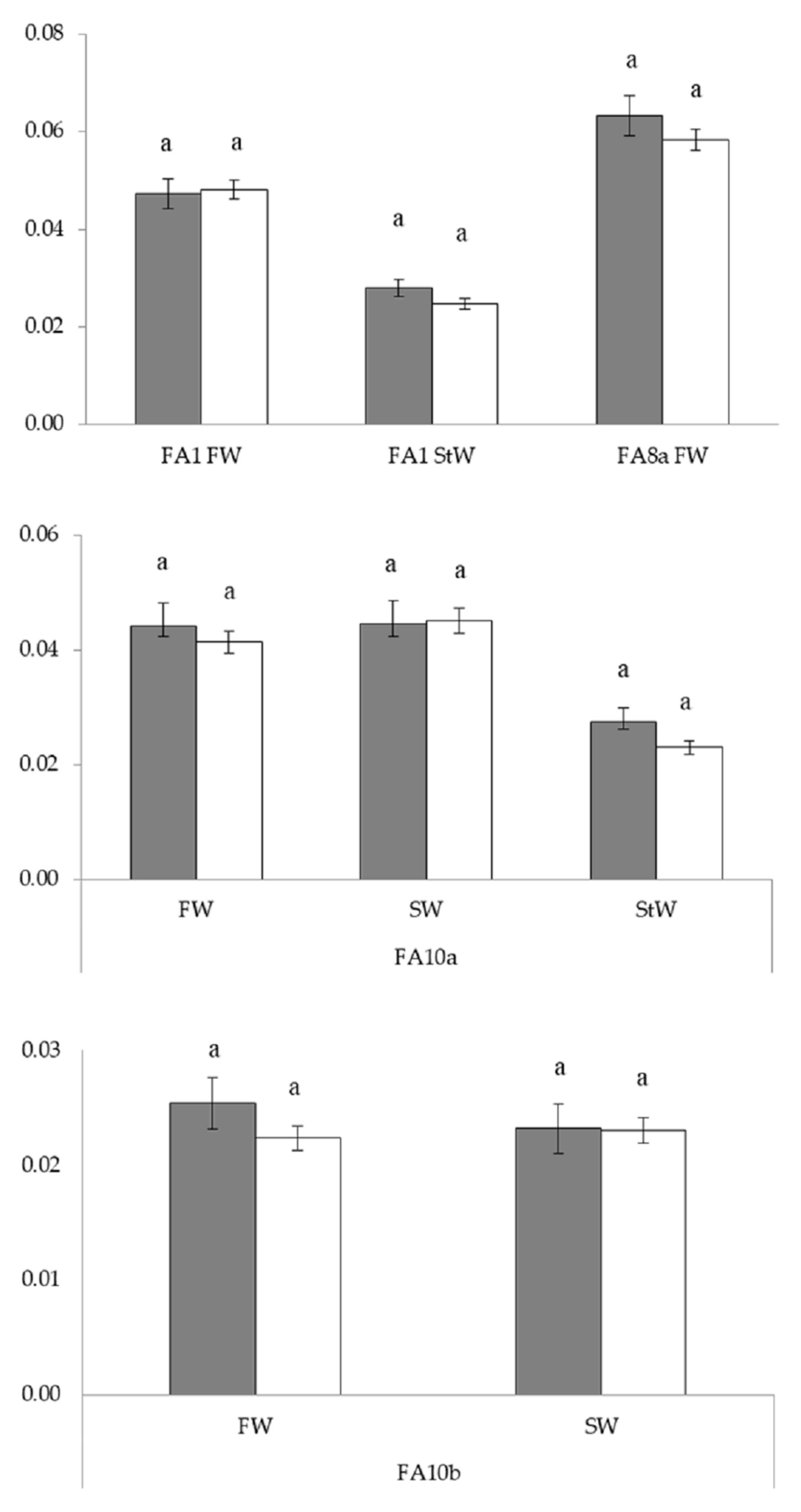
| Univariate FA | FA1 FW | FA1 StW | FA8a FW | |||||||
|---|---|---|---|---|---|---|---|---|---|---|
| df | MS (10−3) | F | df | MS (10−3) | F | df | MS (10−3) | F | ||
| S | 1 | 0.03 | 0.02 ns | 1 | 1.22 | 2.48 ns | 1 | 4.05 | 1.30 ns | |
| C | 56 | 1.94 | 1.46 * | 55 | 0.52 | 1.26 ns | 56 | 2.73 | 1.31 ns | |
| S × C | 52 | 1.69 | 1.28 ns | 49 | 0.49 | 1.19 ns | 52 | 3.12 | 1.50 * | |
| F(S × C) | 200 | 1.53 | 1.16 ns | 174 | 0.47 | 1.13 ns | 200 | 2.31 | 1.11 ns | |
| Error | 598 | 1.33 | 524 | 0.42 | 598 | 2.08 | ||||
| FW | SW | StW | ||||||||
| df1/df2 | F | df1/df2 | F | df1/df2 | F | |||||
| FA10a | ||||||||||
| S | 119/707 | 1.07 ns | 182/651 | 0.99 ns | 181/621 | 1.19 ns | ||||
| FA10b | ||||||||||
| S | 119/707 | 1.37 ns | 182/651 | 1.01 ns | 181/621 | 1.20 ns | ||||
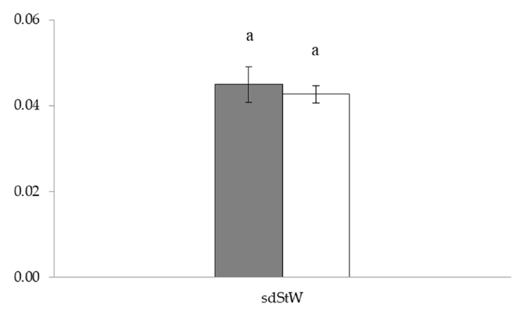
| Univariate RA | sd StW | |||||||||
| df | MS (10−3) | F | ||||||||
| S | 1 | 0.34 | 0.23 ns | |||||||
| C | 55 | 1.21 | 1.59 * | |||||||
| S × C | 49 | 1.50 | 1.98 ** | |||||||
| Error | 280 | 0.76 | ||||||||
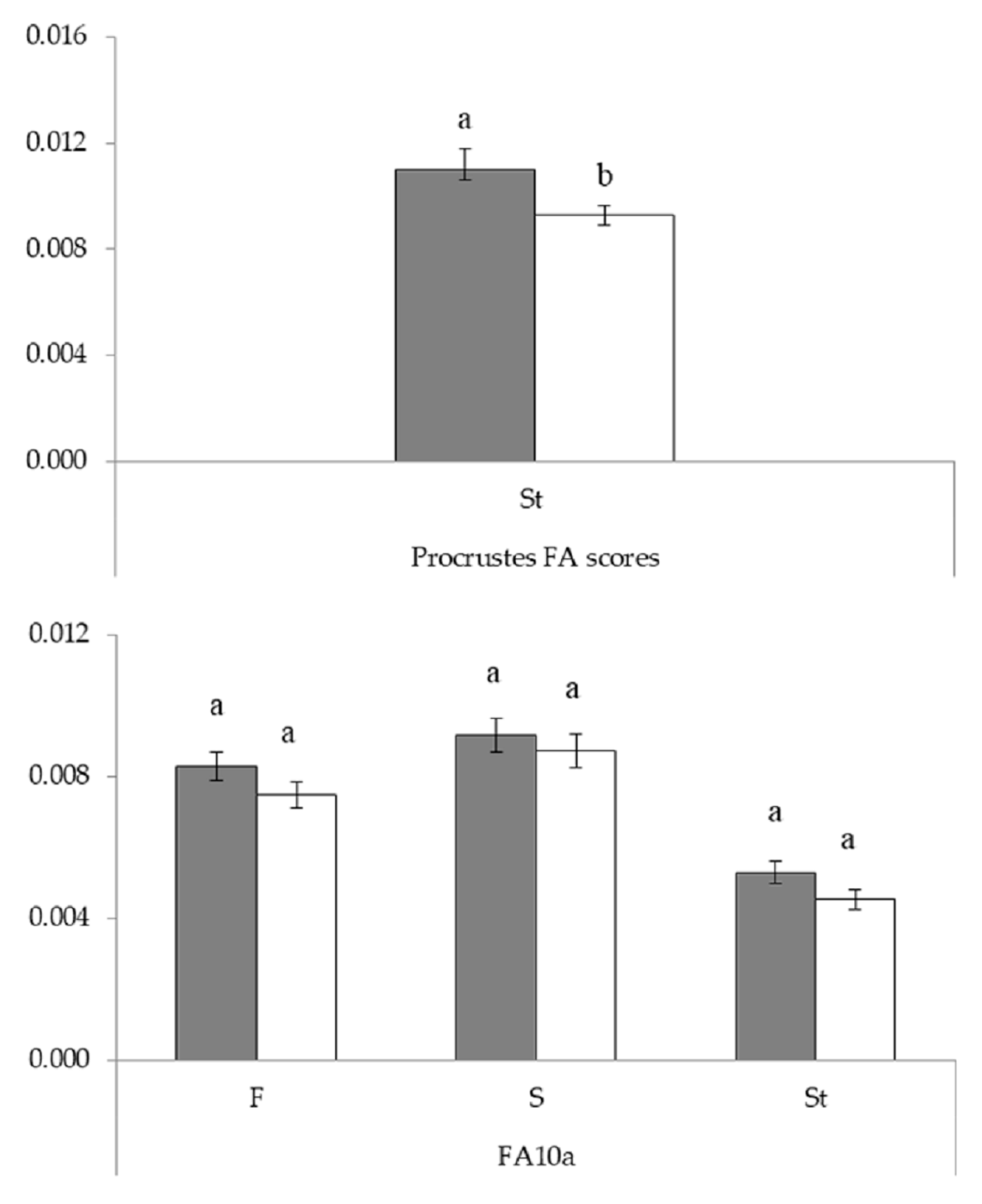
| Shape FA | F | S | St | ||||
|---|---|---|---|---|---|---|---|
| FA10a Site | df1/df2 | F | df1/df2 | F | df1/df2 | F | |
| 594/605 | 1.11 ns | 614/550 | 1.05 ns | 378/392 | 1.16 ns | ||
| Shape RA | St | ||||||
| df | MS (10−6) | F | |||||
| Site | 1 | 81.28 | 4.00 * | ||||
| Error | 110 | 20.31 | |||||
© 2019 by the authors. Licensee MDPI, Basel, Switzerland. This article is an open access article distributed under the terms and conditions of the Creative Commons Attribution (CC BY) license (http://creativecommons.org/licenses/by/4.0/).
Share and Cite
Barišić Klisarić, N.; Miljković, D.; Avramov, S.; Živković, U.; Tarasjev, A. Radial and Bilateral Fluctuating Asymmetry of Iris pumila Flowers as Indicators of Environmental Stress. Symmetry 2019, 11, 818. https://doi.org/10.3390/sym11060818
Barišić Klisarić N, Miljković D, Avramov S, Živković U, Tarasjev A. Radial and Bilateral Fluctuating Asymmetry of Iris pumila Flowers as Indicators of Environmental Stress. Symmetry. 2019; 11(6):818. https://doi.org/10.3390/sym11060818
Chicago/Turabian StyleBarišić Klisarić, Nataša, Danijela Miljković, Stevan Avramov, Uroš Živković, and Aleksej Tarasjev. 2019. "Radial and Bilateral Fluctuating Asymmetry of Iris pumila Flowers as Indicators of Environmental Stress" Symmetry 11, no. 6: 818. https://doi.org/10.3390/sym11060818