Mean-Field Expansion, Regularization Issue, and Multi-Quark Functions in Nambu–Jona-Lasinio Model

Abstract

In this paper, the results of the investigation of multi-quark equations in the Nambu–Jona-Lasinio (NJL) model in the mean-field expansion are presented. The multi-quark functions have been considered up to the third order of expansion. One of the purposes of our computations is the study of corrections of higher orders to parameters of the model. The important problem of the application of the NJL model is regularization. We compare the NJL model with 4-dimensional cutoff regularization and the dimensionally analytical regularization. We also discuss so-called “predictive regularization” in the NJL model, and a modification of this regularization, which is free of the Landau pole, is proposed. To calculate the high-order corrections, we use the Legendre transform method in the framework of bilocal-source formalism, which allows one effectively to take into consideration the symmetry constraints. A generalization of the mean-field expansion for other types of multi-quark sources is also discussed.

1. Introduction

Quantum chromodynamics as the theory of strong interactions has achieved great successes in the description of various hadronic processes. Due to the asymptotic freedom of this theory it explains processes at short distances. However, for the quantitative description of the region of intermediate and large distances, simplified effective models are necessary.

In 1961, Nambu and Jona-Lasinio [1] constructed a superconducting-type model based on four-fermion interaction for understanding a nucleon mass nature and a mechanism of spontaneous breaking of chiral symmetry.

Eguchi [2] and Kikkawa [3] reformulated the Nambu–Jona-Lasinio (NJL) model for quark fields (see also [4,5]). Hatsuda and Kunihiro [6] used an improved NJL model for description of dense and hot media of hadrons. This model can be applied to study light nuclei as well. The NJL model is currently the most successful model of quantum chromodynamics in non-perturbative region (see [7,8,9,10,11,12] for reviews and further references).

The applications of NJL model in recent years, has intensified in various problems of nuclear physics and a cosmology (see [13,14,15,16,17,18,19,20,21,22,23,24,25,26,27,28,29] and references therein). Of great interest is the generalization of the NJL model, which contains the quark confinement mechanism (the so-called Polyakov-loop extended Nambu–Jona-Lasinio model, or PNJL model; see, for example [22] and references therein). Consideration of this model, however, is beyond the scope of our work.

Among applications of phenomenological models are investigations of multi-quark functions, which are main topic of the present work. The formalism of multilocal sources are basic idea behind of this approach [30,31]. The method of multilocal sources has been used in various field-theoretical studies and may be employed for similar calculations in effective model as well [32,33].

The multi-quark functions appear in the mean-field expansions (MFE) of the NJL model in higher-order terms. To obtain the MFE the iteration scheme of the Schwinger-Dyson solutions with the bilocal fermion source have been used [32,33]. This iterative approach is fruitful because equations under discussion have a simple structure, and the solution of these equations at all orders is an algebraic problem. In this work we consider equations for correlation functions of the NJL model up to the third order of MFE. The leading order (LO) and a first step of this scheme include the equations for the quark propagator, the two-quark function and the next-to-leading (NLO) correction to the quark propagator. The second order of MFE includes the equations for the four-quark and the three-quark functions and the equations for the NLO two-quark function and next-to-next-to-leading order (NNLO) quark propagator.

We have solved the four-quark and three-quark equations. The third step of iterations, which includes equations for the six-quark and five-quark functions and the equations for the NLO four-quark and three-quark functions, is also investigated.

The NJL model in the MFE contains quark loops and corresponding ultraviolet divergences. Therefore, regularization procedure is the essential point for this model. Traditionally used regularizations for the NJL model are based on a four-dimensional (4D) cutoff in Euclidean momenta or a three-dimensional momentum cutoff. The Pauli-Villars regularization, or non-local Gauss form-factors, are also used. However, the most popular and very convenient for calculations dimensional regularization is the least used for the NJL model. The reason is related to the next issue: a regularizations parameter for NJL model is involved in physical quantities. Therefore, it is the essential parameter for NJL model. However, the parameter of dimensional regularization is a deviation from the physical dimension of space, which cannot be connected directly with any physical quantity.

An alternative approach is a consideration of the dimensional regularization as a variant of the analytical regularization. In framework of this treatment all computations are made in 4D Euclidean momentum space. For regularization of the divergent integrals, a weight function into integrand is included, and the regularization parameter is a power of this function. This variant of dimensional regularization is consistently developed and applied to the NJL model by Krewald and Nakayama [34]. The parameter of such regularization is not at all a deviation from the physical dimension of space. We assume that this parameter can be treated as a “trace of gluons” in the effective four-quark self-action of NJL model. Such treatment in some sense is similar to the non-local versions of the NJL model.

In our paper we analyze the dimensional regularization in the NLO of the MFE in the frame of Krewald and Nakayama approach. (We introduce the new term “dimensionally analytical regularization” (DAR) for avoiding an unnecessary association with the traditional dimensional regularization).

An interesting attempt for a deliverance of the NJL model from the regularization dependence made in the work of Battistel, Dallabona and Krein (BDK) [35] (see also [36,37]). Main idea of the method, named by authors as “predictive regularization”, consists of a separation of the finite parts of divergent integrals from the divergent ones, and then the integration is done without regularization. A significant result of work [35] is a proof of the fulfillment of symmetry constraints for correlation functions. We discuss some features of the computational scheme of work [35]. The main problem of this method is the singularity of meson propagators in the region of Euclidean momenta. The existence of these Landau singularities is an essential problem for any computations beyond the leading approximation. A modification of this scheme is proposed, which is free from Landau poles and conserves the main features of the approach of [35] (see also [38,39,40]).

The structure of the paper is following. In Section 2 we construct MFE in the fermion bilocal-source formalism. The DAR of the NJL model is discussed in Section 3. The predictive regularization and the problem of Landau ghost is discussed in Section 4.

A purpose of our computations is to study the corrections of higher orders to parameters of the model, such as the chiral condensate and pion-decay constant. The sigma-meson and pion contributions to the chiral quark condensate are considered in Section 5. The chiral condensate is the principal order parameter of dynamical chiral symmetry breaking (DCSB). As our computations demonstrate, the pion contribution to chiral condensate is inversely proportional to the regularization parameter of DAR and is independent of other parameters of the model. The sigma-meson contribution is small for admissible values of the parameter (see [41,42,43]).

In Section 6 we investigate the corrections to the two-quark function by the method of the Legendre transform with respect to the bilocal source [30,31]. As is shown, this method is an effective way to take into account the constraints following from the chiral Ward identity (see also [44]).

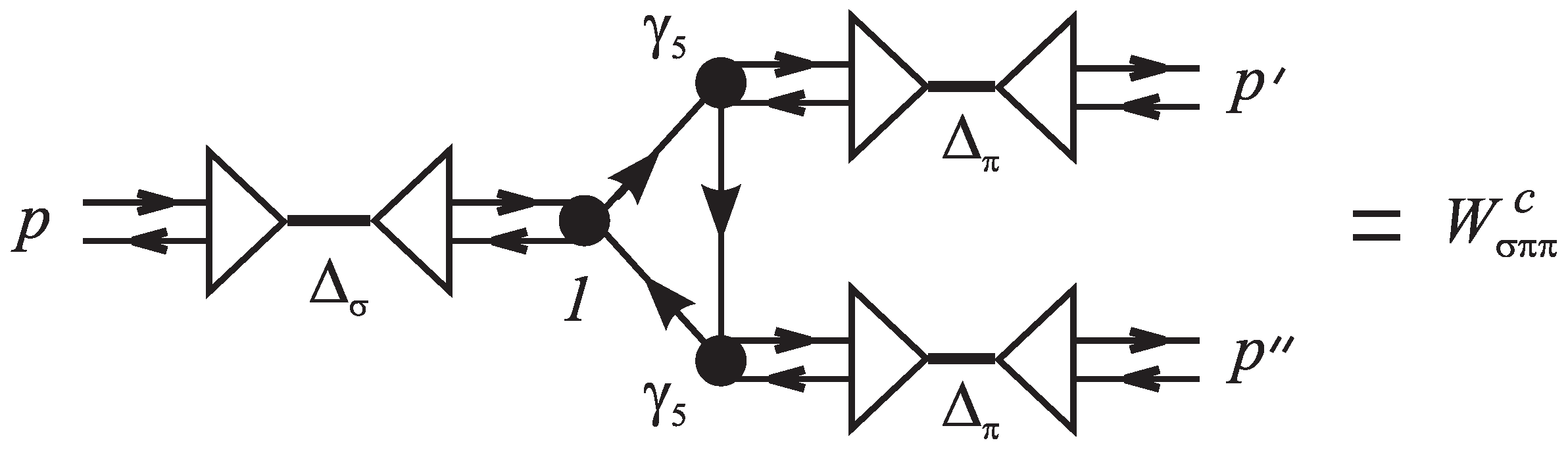
In Section 7 we consider the higher orders of the iteration scheme. We calculate the three-quark function, which describes the decay $\sigma \to \pi \pi$ and a correction to pion-decay constant.

In Section 8 the generalization of the MFE for the NJL model in the framework of the diquark and triple-quark sources formalism is shortly discussed. Such generalization can be fruitful, in particular, for the quantum-field description of nucleons.

2. The Mean-Field Expansion in the Bilocal-Source Formalism

Let us consider the chiral-symmetric NJL model. The model is based on u and d quark fields $\psi \left(x\right)$. The two-flavor NJL model Lagrangian is

$$L=\overline{\psi }i\widehat{\partial }\psi +\frac{g}{2}\left[{\left(\overline{\psi }\psi \right)}^2+{\left(\overline{\psi }i{\gamma }_5{\tau }^a\psi \right)}^2\right],$$

(1)

where g is the four-fermion coupling constant with the mass dimension $m^{-2}$. Here we omit the bare masses of u and d quarks which are much smaller than the QCD scale. The chiral $S{U}_V\left(2\right)\times S{U}_A\left(2\right)$ invariance prohibits a mass term in the Lagrangian. In Equation (1) $\psi \equiv {\psi }_j^{\alpha c}$, where $\alpha =1,2,3,4$, $c=1,\dots ,N_c$ and $j=1,2$ are spinor, color and isotopic (flavor) indexes correspondingly, and $\widehat{\partial }\equiv {\gamma }^{\mu }{\partial }_{\mu }$. The $SU\left(2\right)$-group generators ${\tau }^a$ are normalized as $tr\left({\tau }^a{\tau }^b\right)=2{\delta }^{ab}$.

The generating functional G of vacuum expectation values of T-products of fields (correlation functions) can be written as the following functional integral with bilocal quark-antiquark source $\eta$:

$$G\left(\eta \right)=\int d(\psi ,\overline{\psi })expi\left\{\int dxL-\int dxdy\overline{\psi }\left(y\right)\eta (y,x)\psi \left(x\right)\right\}.$$

(2)

The n-th functional derivation with respect to source $\eta$ of generating functional G is the $2n$-point (n-particle) function:

$$\frac{{\delta }^{n}G}{\delta \eta (y_1,x_1)\cdots \delta \eta (y_n,x_n)}{|}_{\eta =0}=i^n<0\mid T\left\{\psi \left(x_1\right)\overline{\psi }\left(y_1\right)\cdots \psi \left(x_n\right)\overline{\psi }\left(y_n\right)\right\}\mid 0>\equiv S_n\left(\begin{array}{cc}{x}_1& y_1\\ \cdots & \cdots \\ x_n& y_n\end{array}\right).$$

The translational invariance of the functional integration measure implies relation

$$\int d(\psi ,\overline{\psi })\frac{\delta }{\delta \overline{\psi }\left(x\right)}\overline{\psi }\left(y\right)exp\left\{\int dxL\left(x\right)-\int dxdy\overline{\psi }\left(x\right)\eta (x,y)\psi \left(y\right)\right\}=0,$$

that can be written as the functional-differential Schwinger–Dyson equation (SDE):

$$\delta (x-y)G+i{\widehat{\partial }}_x\frac{\delta G}{\delta \eta (y,x)}+ig\left\{\frac{\delta }{\delta \eta (y,x)}tr\left[\frac{\delta G}{\delta \eta (x,x)}\right]-{\gamma }_5{\tau }^a\frac{\delta }{\delta \eta (y,x)}tr\left[{\gamma }_5{\tau }^a\frac{\delta G}{\delta \eta (x,x)}\right]\right\}$$

$$=\int d{x}_1\eta (x,x_1)\frac{\delta G}{\delta \eta (y,x_1)}.$$

(3)

To formulate the MFE we shall use the procedure which was proposed in Reference [45]. A leading approximation is the SDE (3) with zero r.h.s.:

$$G^{\left(0\right)}+i{\widehat{\partial }}_x\frac{\delta G^{\left(0\right)}}{\delta \eta }+ig\left\{\frac{\delta }{\delta \eta }tr\left[\frac{\delta G^{\left(0\right)}}{\delta \eta }\right]-{\gamma }_5{\tau }^a\frac{\delta }{\delta \eta }tr\left[{\gamma }_5{\tau }^a\frac{\delta G^{\left(0\right)}}{\delta \eta }\right]\right\}=0.$$

The solution of the leading approximation equation is the functional

$$G^{\left(0\right)}=exp\left\{\mathrm{T}\mathrm{r}\left(S\ast \eta \right)\right\},$$

where $\mathrm{T}\mathrm{r}$ is the operator trace and ∗ is the multiplication of operators. A function S (quark propagator) in above formula for $G^{\left(0\right)}$ is the solution of following equation

$$\delta \left(x\right)+i\widehat{\partial }S\left(x\right)+igS\left(x\right)tr\left[S\left(0\right)\right]=0.$$

(4)

The leading approximation produces the linear iteration procedure in which the term with bilocal source $\eta$ must be considered to be perturbation [32,33]. Thus, we can construct the iteration scheme for generating functional G

$$G=G^{\left(0\right)}+G^{\left(1\right)}+\cdots +G^{\left(n\right)}+\cdots .$$

This series consists of the step-by-step solutions of the following equations

$$G^{\left(n\right)}+i{\widehat{\partial }}_x\frac{\delta G^{\left(n\right)}}{\delta \eta }+ig\left\{\frac{\delta }{\delta \eta }tr\left[\frac{\delta G^{\left(n\right)}}{\delta \eta }\right]-{\gamma }_5{\tau }^a\frac{\delta }{\delta \eta }tr\left[{\gamma }_5{\tau }^a\frac{\delta G^{\left(n\right)}}{\delta \eta }\right]\right\}=\eta \ast \frac{\delta G^{(n-1)}}{\delta \eta }.$$

(5)

The functional $G^{\left(n\right)}$ is

$$G^{\left(n\right)}=P^{\left(n\right)}{G}^{\left(0\right)}.$$

Here $P^{\left(n\right)}$ are $2n$ -th degree polynomials on bilocal source $\eta$.

Leading-order correlator S is a quark propagator (a single-particle function). It is

$$S_{cd,jk}={\delta }_{cd}{\delta }_{jk}{(m-\widehat{p})}^{-1},$$

(6)

where m is the dynamical quark mass that is a solution of the gap equation of the NJL model in the chiral limit

$$m=-8igm{N}_c\int \frac{d\tilde{q}}{m^2-q^2}.$$

(7)

(In our work, we include a phase factor in an integration over momentum space $d\tilde{q}\equiv d^{4}q/{\left(2\pi \right)}^4$). The basic order parameter, which defines a degree of DCSB, is a quantity

$$\chi =<0|\overline{\psi }\psi {|0>=itrS\left(x\right)|}_{x\to 0},$$

where we take the trace over all discrete indices. It is easy to see that from Equations (6) and (7) it follows

$$\chi =-\frac{m}{g}.$$

(8)

It is a regularization-independent formula.

The quark chiral condensate c is defined for each flavor separately and in the chiral limit considered here it is

$$c={\left(\frac{\chi }{2}\right)}^{1/3}.$$

(9)

Equation (7) is the main equation, which describes the principal phenomenon of NJL model—DCSB. The divergent integral in Equation (7) should be considered to be a regularization (see Section 3).

2.1. First-Step Equations

In this subsection we discuss the structure of first step of iteration scheme.

Gap Equation (7) always has the chiral-symmetric trivial solution $m=0$. An energetically preferable physical solution $m\ne 0$, i.e., a solution with DCSB also exists, and below we shall consider a solution at $m\ne 0$ only.

The functional of the first step of iteration scheme can be represented as

$$G^{\left(1\right)}=\left\{\frac{1}{2}\mathrm{T}\mathrm{r}\left(S_2\ast {\eta }^2\right)+\mathrm{T}\mathrm{r}\left(S^{\left(1\right)}\ast \eta \right)\right\}{G}^{\left(0\right)}.$$

(10)

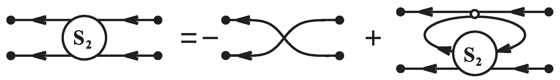
In this step two-quark function $S_2$ and NLO correction $S^{\left(1\right)}$ to quark propagator emerge.

According to Equation (5) at $n=1$ we obtain for two-particle functions $S_2$ and NLO correction to quark propagator $S^{\left(1\right)}$ following equations:

$$S_2\left(\begin{array}{cc}x& y\\ x^{\prime }& y^{\prime }\end{array}\right)=-S(x-y^{\prime })S(x^{\prime }-y)$$

$$+ig\int d{x}_1\{\left(S(x-x_1)S(x_1-y)\right)t{r}_u\left[S_2\left(\begin{array}{cc}{x}_1& x_1\\ x^{\prime }& y^{\prime }\end{array}\right)\right]$$

$$-\left(S(x-x_1){\gamma }_5{\tau }^{a}S(x_1-y)\right)t{r}_u\left[{\gamma }_5{\tau }^a{S}_2\left(\begin{array}{cc}{x}_1& x_1\\ x^{\prime }& y^{\prime }\end{array}\right)\right]\},$$

(11)

(here and hereafter $t{r}_u$ denotes the upper line trace of functions $S_2$) and

$$S^{\left(1\right)}(x-y)=ig\int d{x}_{1}S(x-x_1)\left\{S_2\left(\begin{array}{cc}{x}_1& y\\ x_1& x_1\end{array}\right)-{\gamma }_5{\tau }^a{S}_2\left(\begin{array}{cc}{x}_1& y\\ x_1& x_1\end{array}\right){\gamma }_5{\tau }^a\right\}$$

$$+ig\int d{x}_{1}S(x-x_1)S(x_1-y)tr\left[S^{\left(1\right)}\right]\left(0\right).$$

(12)

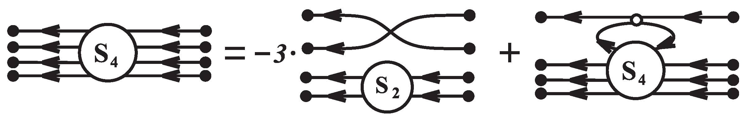
These equations are reduced in the momentum space to a system of simple algebraic forms. The graphical representations of two-quark function see on Figure 1, where the graphical notations of Figure 2 are used.

2.2. Pion and Sigma-Meson

Let us go to the amputated two-quark function

$$F_2=S^{-1}\ast S^{-1}\ast S_2\ast S^{-1}\ast S^{-1},$$

(13)

and separate the connected part of $F_2$

$$F_2^c\left(\begin{array}{cc}x& y\\ x^{\prime }& y^{\prime }\end{array}\right)=F_2\left(\begin{array}{cc}x& y\\ x^{\prime }& y^{\prime }\end{array}\right)+S^{-1}(x-y^{\prime })S^{-1}(x^{\prime }-y).$$

(14)

As a result of this procedure we get following equation for two-quark function $F_2^c$:

$$F_2^c\left(\begin{array}{cc}x& y\\ x^{\prime }& y^{\prime }\end{array}\right)=-ig\delta (x-y)\delta (x-y^{\prime })\delta (x^{\prime }-y)\{1·1-{\gamma }_5{\tau }^a·{\gamma }_5{\tau }^a\}$$

$$+ig\delta (x-y)\int d{x}_{1}d{y}_1\{t{r}_u\left[S(x-x_1)F_2^c\left(\begin{array}{cc}{x}_1& y_1\\ x^{\prime }& y^{\prime }\end{array}\right)S(y_1-y)\right]$$

$$-{\gamma }_5{\tau }^{a}t{r}_u\left[{\gamma }_5{\tau }^{a}S(x-x_1)F_2^c\left(\begin{array}{cc}{x}_1& y_1\\ x^{\prime }& y^{\prime }\end{array}\right)S(y_1-y)\right]\}.$$

(15)

Accounting the color, flavor, and Lorentz structures of the inhomogeneous term of this equation we obtain the general form of solution

$$F_2^c\left(\begin{array}{cc}x& y\\ x^{\prime }& y^{\prime }\end{array}\right)=\delta (x-y)\delta (x^{\prime }-y^{\prime })\{1·1A_{\sigma }(x-x^{\prime })+{\gamma }_5{\tau }^a·{\gamma }_5{\tau }^a{A}_{\pi }(x-x^{\prime })\},$$

(16)

where $A_{\sigma }$ and $A_{\pi }$ are the sigma meson (scalar) and pion (pseudoscalar) amplitudes, correspondingly. These are the solutions of the following equations

$$A_{\sigma }\left(x\right)=-ig\delta \left(x\right)+ig\int d{x}_{1}tr\left[S(x-x_1)S(x_1-x)\right]A_{\sigma }\left(x_1\right),$$

(17)

$$A_{\pi }\left(x\right)=ig\delta \left(x\right)-ig\int d{x}_{1}tr\left[{\gamma }_{5}S(x-x_1){\gamma }_{5}S(x_1-x)\right]A_{\pi }\left(x_1\right).$$

(18)

Going to the momentum space and accounting for gap Equation (7), one gets

$$A_{\sigma }\left(p\right)=\frac{1}{4N_c(4m^2-p^2)I_0\left(p\right)}$$

(19)

and

$$A_{\pi }\left(p\right)=\frac{1}{4N_c{p}^2{I}_0\left(p\right)}.$$

(20)

Here

$$I_0\left(p\right)=\int d\tilde{q}\frac{1}{(m^2-{(p+q)}^2)(q^2-m^2)}$$

(21)

is the divergent single-loop integral that should be treated as some regularization.

The scalar and pseudoscalar amplitudes, as can be observed in Equations (19) and (20), contain the simple poles, which indicate to the scalar particle with mass $2m$ (the sigma-meson) and to the massless pseudoscalar particle (pion). Such appearance of the pseudoscalar massless particle (Goldstone boson) in the spectrum has agree with the general Nambu-Goldstone-Bogoliubov (NGB) theorem.

From equation $S^{\left(1\right)}$ (12) for the NLO correction to quark propagator we can calculate the meson corrections to quark mass. This equation is transformed in the momentum space to a system of simple algebraic forms, which contain the NLO mass operator ${\mathsf{\Sigma }}^{\left(1\right)}=S^{-1}\ast S^{\left(1\right)}\ast S^{-1}$. We obtain from (12):

$${\mathsf{\Sigma }}^{\left(1\right)}\left(x\right)=S\left(x\right)A_{\sigma }\left(x\right)+3S(-x)A_{\pi }\left(x\right)+ig\delta \left(x\right)tr\left[S^{\left(1\right)}\left(0\right)\right].$$

(22)

3. Regularization Issue: DAR

The NJL model is based on the unrenormalized 4-fermion contact interaction, and the choice of the regularization scheme is an important issue in the effective use of this model. The integral $I_0$ in frameworks of different regularizations is finite for $P^2=4m^2$ and for $P^2=0$, (see, e.g., [8] for review) (The NJL model as the effective model of QCD is based on the color-current expansion and the Fierz transformation of the one-gluon exchange interaction (see, for example, [9] and references therein). Such approach implies the presence of some parameter which regulates the ultraviolet properties of the model. For this reason, a regularization with momentum cutoff seems to be very natural for this model. Other regularizations, although they do not have such a transparent physical interpretation, in some cases can be more convenient for computations or for the taking into account some special properties of the model), but a most popular gauge-invariant dimensional regularization should be used in this model with some special treatment.

We study in this section the NJL model with dimensional regularization in approach of Krewald and Nakayama [34] (see also [45,46,47,48,49,50,51]). Contrary to renormalized models, a regularization parameter of the NJL model is involved in formulas for observable quantities. This parameter is one of the essentials for the NJL model. However, dimensional regularization parameter, which typically is taken as a deviation of space dimension, does not allow any physical interpretation. Nevertheless, a different approach to the dimensional regularization exists: it can be considered as a variant of an analytical regularization. In this approach all calculations are made in 4D Euclidean momentum space, and the regularization parameter is treated as a power of a weight function, which regularizes divergent integrals. This approach to the dimensional regularization, based on ideas of Wilson and Collins, was consistently developed and applied to the NJL model by Krewald and Nakayama [34] in the mean-field approximation. We stress that in this treatment of dimensional regularization, the regularization parameter is not at all a deviation in the physical dimension of space.

The general characteristics of the approach are:

(i)

All computations are made in 4D Euclidean space;

(ii)

Translational invariance is supposed;

(iii)

The regularization procedure includes of modification of integration measure via the weight function which provides the convergence of integrals.

In this connection we shall use the term “dimensionally analytical” for this regularization to stress its properties which differ from the conventional approach of the dimensional regularization in a formal D-dimensional space.

Let us study of the NJL model gap Equation (7) for example. After performing integration by angles, the gap equation in the case $m\ne 0$ in Euclidean space is

$$2g\frac{{\mathsf{\Omega }}_4}{{\left(2\pi \right)}^4}\int \frac{q_e^{2}d{q}_e^2}{m^2+q_e^2}=1,$$

where ${\mathsf{\Omega }}_4=2{\pi }^2$. Let us (according the previous comment) include to the integrand the weight function

$$w_{\mathsf{\Lambda },D}\left(q_e^2\right)=w_{\mathsf{\Lambda }}\left(q_e^2\right)w_D\left(q_e^2\right)=\theta ({\mathsf{\Lambda }}^2-q_e^2)(\frac{{\mu }^2}{q_e^2}{)}^{2-D/2}.$$

The weight function $w_{\mathsf{\Lambda },D}$ is the product of two weight functions $w_{\mathsf{\Lambda }}$ and $w_D$. The first function $w_{\mathsf{\Lambda }}$ corresponds to the 4D cutoff regularization, and the second power function $w_D$ conforms to DAR.

The integration over $d{q}_e^2$ results in

$$\frac{2g{m}^2{\mathsf{\Omega }}_4}{{\left(2\pi \right)}^4}(\frac{m^2}{{\mu }^2}{)}^{D/2-2}{B}_{\frac{{\mathsf{\Lambda }}^2}{m^2+{\mathsf{\Lambda }}^2}}(D/2,1-D/2)=1.$$

Here $B_x(u,v)$—the incomplete Beta-function.

(a) Cutoff: By setting $D=4$, we have the following result:

$${\kappa }_{\mathsf{\Lambda }}(1-\frac{m^2}{{\mathsf{\Lambda }}^2}log(1+\frac{{\mathsf{\Lambda }}^2}{m^2}))=1,$$

(23)

where

$${\kappa }_{\mathsf{\Lambda }}=\frac{g{N}_c{\mathsf{\Lambda }}^2}{2{\pi }^2}.$$

(24)

(b) Dimensionally analytical regularization: When ${\mathsf{\Lambda }}^2\to \infty$, accounting for the formula $B_1(D/2,1-D/2)=\mathsf{\Gamma }(D/2)\mathsf{\Gamma }(1-D/2)$ and rescaling the scale parameter ${\mu }^2$ as

$${\left({\mu }^2\right)}^{2-D/2}=\frac{{\mathsf{\Omega }}_D}{{\mathsf{\Omega }}_4}\frac{{\left(2\pi \right)}^4}{{\left(2\pi \right)}^D}{\left(M\right)}^{2-D/2}$$

(25)

we obtain

$$\kappa \mathsf{\Gamma }(1-D/2)(\frac{m^2}{4\pi M^2}{)}^{D/2-2}=1,$$

(26)

where instead of g we introduce the dimensionless quantity

$$\kappa =\frac{g{N}_c{m}^2}{2{\pi }^2}.$$

(27)

Formula (26) corresponds exactly to the result of integration in D-dimensional space with the prescription

$$d\tilde{q}\equiv \frac{d^{4}q}{{\left(2\pi \right)}^4}\to \frac{{\left(M^2\right)}^{2-D/2}{d}^{D}q}{{\left(2\pi \right)}^D},$$

however, in our situation the computation was performed in the usual 4D space, i.e., in our case D is not a dimension of space. It is a parameter which enables the convergence. In particular, we are not restricted by the limit $D\to 4$ for the analysis of the results. We assume that a possible technique of regularization parameter is a power of some supplementary factor—the measure of gluon influence on the effective local 4-quark self-interaction of the NJL model.

We choose the regularization parameter $\xi$ as: (The parameter $\xi$ differs from the typically used parameter $\epsilon =(4-D)/2.$ They are related as $\epsilon =1+\xi$. Introduction of this notation protect unnecessary associations with the usual definition of the dimensional regularization.)

$$D=2-2\xi .$$

(28)

In terms of the parameter $\xi$ the gap Equation (26) is

$$\kappa \mathsf{\Gamma }\left(\xi \right)(\frac{4\pi M^2}{m^2}{)}^{1+\xi }=1.$$

(29)

The interval of convergence of the integral is $0<\xi <1.$ As we shall see below, this is also the interval of the physical values of the model parameters.

The LO chiral condensate correspondingly is

$${\left(c^3\right)}^{\left(0\right)}=itrS\left(0\right)=-\frac{m^3}{4{\pi }^2}(\frac{4\pi M^2}{m^2}{)}^{1+\xi }\mathsf{\Gamma }\left(\xi \right)=-\frac{m}{g}.$$

Two-Quark Amplitude and Model Parameters in Leading Approximation

First-step two-quark amplitude A (a connected part of amputated two-quark function) possesses the following color and flavor structure:

$$A_{c^{\prime }{d}^{\prime },j^{\prime }{k}^{\prime }}^{cd,jk}={\delta }^{cd}{\delta }^{c^{\prime }{d}^{\prime }}\left[{\delta }_{jk}{\delta }_{j^{\prime }{k}^{\prime }}{A}_{\sigma }+{\tau }_{jk}^a{\tau }_{j^{\prime }{k}^{\prime }}^a{A}_{\pi }\right].$$

(30)

Here $A_{\sigma }$ is the scalar amplitude, and $A_{\pi }$ is the pseudoscalar amplitude. In momentum space these amplitudes of the NJL model depend on a momentum p only, where p is a sum of quark and antiquark momenta. They have the form [46]:

$$A_{\sigma }\left(p\right)=-\frac{ig}{1-L_S\left(p\right)},$$

(31)

where $L_S\left(p\right)=ig\int d\tilde{q}trS(p+q)S\left(q\right)$ is the scalar quark loop, and

$$A_{\pi }\left(p\right)=\frac{ig}{1+L_P\left(p\right)},$$

(32)

where $L_P\left(p\right)=ig\int d\tilde{q}trS(p+q){\gamma }_{5}S\left(q\right){\gamma }_5$ is the pseudoscalar quark loop.

Using simple algebra and gap Equation (7), it is easy to obtain for $A_{\sigma }$ and $A_{\pi }$ in above-mentioned representations (19) and (20), where integral $I_0$ (see (21)) can be calculated as above. Going to Euclidean space, using a Feynman parameterization and changing an integration variable (which is possible due to translational invariance of the procedure), we perform the angular integration. According to our prescriptions, then we introduce into the integrand a weight function and calculate the integral over $d{q}_e^2$. For DAR we again obtain the result, which exactly corresponds to the result of integration with the formal transition to D-dimensional space:

$$I_0^{DAR}\left(p^2\right)=\frac{i{\left(4\pi \right)}^{1+\xi }\mathsf{\Gamma }(1+\xi )}{{\left(4\pi \right)}^2}{\int }_0^{1}du{\left(\frac{M^2}{m^2-u(1-u)p^2}\right)}^{1+\xi }.$$

The integral over $d{q}_e^2$ converges at $-1<\xi <1$. Taking into account the gap Equation (29) we obtain:

$$I_0^{DAR}\left(p^2\right)=\frac{i}{{\left(4\pi \right)}^2}\frac{\xi }{\kappa }{\int }_0^{1}du{\left(1-u(1-u)\frac{p^2}{m^2}\right)}^{-1-\xi }=\frac{i}{{\left(4\pi \right)}^2}\frac{\xi }{\kappa }F(1+\xi ,1;3/2;\frac{p^2}{4m^2}),$$

(33)

where $F(a,b;c;z)$ is Gauss hypergeometric function.

For 4D cutoff we correspondingly obtain:

$$I_0^{FDC}\left(p^2\right)=\frac{i}{{\left(4\pi \right)}^2}{\int }_0^{1}du\left[log\left(1+\frac{{\mathsf{\Lambda }}^2}{m^2-u(1-u)p^2}\right)-\frac{{\mathsf{\Lambda }}^2}{{\mathsf{\Lambda }}^2+m^2-u(1-u)p^2}\right].$$

(34)

Formulas for the condensate and the two-particle amplitudes allow to fix values of the model parameters in the leading approximation of MFE. For this purpose, we use regularization-independent Formulas (8), (9) and a formula for pion-decay constant in the NJL model (see [8]):

$$f_{\pi }^2=-4i{N}_c{m}^2{I}_0\left(0\right).$$

(35)

For DAR we obtain from (33):

$$I_0^{DAR}\left(0\right)=\frac{i}{{\left(4\pi \right)}^2}\frac{\xi }{\kappa },$$

(36)

and for 4D cutoff (FDC) (see (34)):

$$I_0^{FDC}\left(0\right)=\frac{i}{{\left(4\pi \right)}^2}\left[log\frac{{\mathsf{\Lambda }}^2+m^2}{m^2}-\frac{{\mathsf{\Lambda }}^2}{{\mathsf{\Lambda }}^2+m^2}\right].$$

(37)

Correspondingly we obtain for DAR very simple formula:

$${\left(f_{\pi }^2\right)}^{DAR}=\frac{\xi }{2g}.$$

(38)

For 4D cutoff the analogous formula is

$${\left(f_{\pi }^2\right)}^{FDC}=\frac{3m^2}{4{\pi }^2}\left[log(1+\frac{{\mathsf{\Lambda }}^2}{m^2})-\frac{{\mathsf{\Lambda }}^2}{m^2+{\mathsf{\Lambda }}^2}\right].$$

(39)

These formulas allow the definition of the values of principal model parameters. We choose the value $f_{\pi }=93$ MeV for the pion-decay constant. Since chiral quark condensate c is not directly measured value, we shall determine sets of parameters for typical values of this quantity. For DAR it is necessary also to fix a value of M (“subtraction point”). In work [45] we have used for this purpose a value of decay width ${\pi }^0\to 2\gamma$. Analysis of results of this work demonstrates that for very large range of condensate values (from −160 to −250 MeV) the value of M is practically permanent and is $M\approx 100$ MeV. Since here we shall take $M=100$ MeV.

The pseudoscalar amplitude associates with the pion, which in the chiral limit is a massless Goldstone boson. In both regularizations under consideration we can define a pion propagator as a pole term of the pseudoscalar amplitude:

$$A_{\pi }^{pole}\left(p\right)=\frac{1}{4N_c{I}_0\left(0\right)p^2},$$

(40)

where $I_0\left(0\right)$ is defined by Equation (36) for DAR and by (37) for 4D cutoff.

The situation is different for the scalar amplitude. Function $I_0\left(p^2\right)$ possesses in both regularizations a cut which originates in the point $p^2=4m^2$. For 4D cutoff it is possible to define a scalar sigma-meson propagator as

$$A_{\sigma }^{pole}\left(p\right)=\frac{1}{4N_c{I}_0\left(4m^2\right)(4m^2-p^2)},$$

(41)

since

$$I_0^{FDC}\left(4m^2\right)=\frac{i}{{\left(4\pi \right)}^2}\left[log\frac{{\mathsf{\Lambda }}^2+m^2}{m^2}+\frac{\mathsf{\Lambda }}{m}arctan\frac{m}{\mathsf{\Lambda }}\right]$$

is a finite quantity. However, for DAR $I_0^{DAR}\left(4m^2\right)$ is finite only at $\xi <-1/2$:

$$I_0^{DAR}\left(4m^2\right){|}_{\xi <-1/2}=-\frac{i}{8g{N}_c{m}^2}\frac{\xi }{1+2\xi }.$$

To interpret the sigma-meson as a particle in the NJL model with DAR we use the following trick: since in the interval $-1<\xi <-1/2$ integral $I_0$ converges we use the value in the point $p^2=m^2$ as a foundation for an analytical continuation of the pole part of the amplitude on parameter $\xi$ to the physical interval $0<\xi <1$. Then the sigma-meson propagator for DAR will be

$${\left(A_{\sigma }^{pole}\left(p\right)\right)}^{DAR}=\frac{2ig{m}^2(1+2\xi )}{(4m^2-p^2)\xi }.$$

(42)

This formula was used for a computation of the sigma-meson contribution in chiral condensate in work [45]. Surely, such procedure of definition of sigma-meson propagator seems to be a somewhat artificial. A more consistent procedure is a separation of a leading singular part of amplitude in the interval of physical values of regularization parameter $\xi$.

The separation of leading singularity near the point $p^2=0$ results for the pseudoscalar amplitude the same result (40), i.e., the pion in DAR possesses all properties of usual observable particle. For the scalar amplitude it is not so. At $p^2\to 4m^2$ we have in interval $0<\xi <1$:

$$I_0^{DAR}\cong \frac{i\sqrt{\pi }\mathsf{\Gamma }(\xi +1/2)}{16g{N}_c{m}^2\mathsf{\Gamma }\left(\xi \right)}{\left(\frac{4m^2}{4m^2-p^2}\right)}^{\xi +1/2},$$

and, correspondingly, the leading singularity is

$${\left(A_{\sigma }^{LS}\right)}^{DAR}\cong -\frac{ig\mathsf{\Gamma }\left(\xi \right)}{\sqrt{\pi }\mathsf{\Gamma }(\xi +1/2)}{\left(\frac{4m^2}{4m^2-p^2}\right)}^{1/2-\xi },$$

(43)

and the leading singularity of scalar amplitude in the model with DAR is of the fundamentally different type in comparison with the cutoff model. Instead of the pole term, which can be naturally interpret as sigma-particle propagator, we obtain for DAR the power behavior which depends on the regularization parameter $\xi$. Thus, we come to the conclusion that for DAR at physical parameter values the scalar amplitude $A_{\sigma }$ does not possess a pole term, which can be interpret as a physical scalar meson.

4. Regularization Issue: Predictive Formulation of the Nambu-Jona-Lasinio Model and Ghost Problem

A very interesting attempt for deliverance the NJL model from the regularization dependence was made in the work [35] (see also [36,37]). The main idea of this approach is to avoid the explicit evaluation of divergent integrals with any specific regularization. The finite parts of integrals are separated of the divergent ones and are integrated without any regularization. Then the NJL model becomes predictive in the sense that its consequences do not depend on the specific regularization of divergent integrals. An important result of work [35] is a proof of the fulfillment of all symmetry constraints. The choice of parameters results in the acceptable values of the quark mass and other parameters of the model.

In this section we analyze some features of this computational scheme We shall name the computational scheme of work [35] as the BDK approach, or the implicit regularization. In particular, we point a connection of the BDK approach with the differential regularization of Gelfand and Shilov [52]. The hard problem of the BDK approach is singularity of meson propagators in the Euclidean region of momenta. The presence of this singularity (Landau pole, or Landau ghost [53]) prevents to any computations beyond the leading approximation. We discuss a modification of the scheme (see also [38,39,40]), which is free of Landau poles and maintains the major features of the BDK approach.

The leading approximation of the model is the mean-field approximation, which coincides with the LO of $1/N_c$–expansion. All correlation functions of the leading approximation are given in terms of single-loop integrals. The problem of computations of these integrals can be transformed to the definition of following five divergent integrals (see [35]):

$$\{I_1;I_1^{\mu }\}=\int d\tilde{k}\frac{\{1;k^{\mu }\}}{{(k+k_1)}^2-m^2},$$

(44)

$$\{I_2;I_2^{\mu };I_2^{\mu \nu }\}=\int d\tilde{k}\frac{\{1;k^{\mu };k^{\mu }{k}^{\nu }\}}{[{(k+k_1)}^2-m^2][{(k+k_2)}^2-m^2]}.$$

(45)

Here m is the dynamical (constituent) quark mass, which is a non-trivial solution of the gap equation for the NJL model.

A basic tool for the definition of integrals (44) and (45) in the BDK approach is an algebraic identity for the propagator function (see Equation (28) in work [35]). With the identity the divergent parts of integrals (44) and (45) have been rewritten via three tensorial and two scalar external-momentum-independent integrals which were treated in the sense of some unspecified regularization. Then integrals (44) and (45) have been represented in terms of these five integrals and two standard convergent integrals (see formulas of section III in work [35]).

In this connection we note some general regularization-independent property of integrals (44) and (45), namely integrals $\{I_1;I_1^{\mu }\}$ and $\{I_2;I_2^{\mu };\}$ are connected with following relations

$$\frac{\partial I_1(k_1;m^2)}{\partial m^2}=I_2(k_1,k_1;m^2)$$

(46)

and

$$\frac{\partial I_1^{\mu }(k_1;m^2)}{\partial m^2}=I_2^{\mu }(k_1,k_1;m^2).$$

(47)

These expressions are regularization-independent and play a significant role in the method. It is not so difficult to verify the validity of these relations for conventional regularization schemes. However, their validity is not evident directly from above-mentioned formulas of work [35]. To prove these relations, we must define derivatives of the external-momentum-independent integrals over $m^2$. For this purpose, we notice that derivatives of logarithmically divergent integrals are convergent integrals and can be calculated without any regularization. This calculation gives us zero value for derivatives of tensorial logarithmically divergent integrals. Then one can verify that the derivatives of quadratically divergent integrals are the corresponding logarithmically divergent integrals. Taking into accounting the circumstance we can easy to derive Equations (46) and (47) for BDK expressions of integrals (44) and (45). Since relations (46) and (47) can be used for alternative definitions of quadratically divergent integrals $I_1$ and $I_1^{\mu }$ without additional regularization, their importance is clear.

Using the expressions (44) and (45) for integrals in work [35], the symmetry constraints on single-loop correlation functions have been analyzed. Based on these relations all symmetry properties of the theory (such as Furry theorem, Ward identities, etc.) can be fulfilled for all single-loop correlation functions. This point is one of the important results of [35]. From the point of view of above discussion the BDK consistency relations simply assert zero values of corresponding integration constants.

The choice of parameters of the NJL model with Lagrangian (1) in the leading approximation is mainly defined by two divergent integrals, namely logarithmically divergent integral $I_2$ and quadratically divergent integral $I_1$. Integral $I_1$ is a part of the gap equation

$$m=-8ig{N}_{c}m·I_1,$$

(48)

which defines dynamical (constituent) quark mass m. Integral $I_2$ determines the structure of meson propagators. Both these integrals can easily be defined with differential regularization without using the above-mentioned algebraic identity for the propagator function.

To define $I_2$ one can use well-known technique of Gelfand and Shilov [52]. Specifically, let us introduce new external variables $p=k_1-k_2$ and $P=k_1+k_2.$ Then derivatives $\partial I_2/\partial p_{\mu }$, $\partial I_2/\partial P_{\mu }$ are convergent integrals, and their computation gives us

$$\frac{\partial I_2}{\partial p_{\mu }}=\frac{i{p}_{\mu }}{16{\pi }^2}{\int }_0^{1}du\frac{u(1-u)}{m^2-u(1-u)p^2},\frac{\partial I_2}{\partial P_{\mu }}=0.$$

(49)

Basing on these results and using identity $p^2\frac{\partial f}{\partial p^2}=\frac{1}{2}{p}_{\mu }\frac{\partial f}{\partial p_{\mu }},$ we naturally go to the following definition:

$$I_2\left(p^2\right)=-\frac{i}{16{\pi }^2}{\int }_0^{1}dulog\frac{m^2-u(1-u)p^2}{m_0^2},$$

(50)

where $m_0$ is the integration constant. This expression coincides with the BDK ones if constant $m_0$ is related to $I_2\left(0\right)$ as

$$I_2\left(0\right)=-\frac{i}{16{\pi }^2}log\frac{m^2}{m_0^2}.$$

(51)

The permutation of two limits—differentiation and regularization removing—is an essential feature of the above computation. Sure, such permutation is implied also in work [35] in the computations of finite parts. This permutation is an essence of Gelfand-Shilov differential regularization [52], which is based on the infinite differentiability of generalized functions.

To define integral $I_1$ we employ regularization-independent relation (46), which gives

$$I_1=\frac{i}{16{\pi }^2}(m^{2}log\frac{m_0^2}{m^2}+m^2-m_1^2),$$

(52)

where $m_1^2$ is the integration constant of Equation (46). This definition also corresponds to BDK ones.

To calculate $m_0$ and $m_1$ and, therefore, to define $I_0$ and $I_1$ in full, we take into account two regularization-independent relations of NJL model, namely

$$f_{\pi }^2=\frac{4N_c{m}^2}{i}{I}_2\left(0\right),$$

(53)

where $f_{\pi }$ is the pion-decay constant, and

$$\chi =2c^3=\frac{8N_{c}m}{i}{I}_1,$$

(54)

where $\chi =<0|\overline{\psi }\psi |0>$ and c is the quark condensate. We have from Equation (53)

$$I_2\left(p^2\right)=\frac{i}{16{\pi }^2}\left[\frac{4{\pi }^2{f}_{\pi }^2}{N_c{m}^2}-{\int }_0^{1}dulog(1-u(1-u)\frac{p^2}{m^2})\right].$$

(55)

Then, using Equations (52) and (54), we obtain for $m_1$

$$m_1^2=m^2+\frac{4{\pi }^2{f}_{\pi }^2}{N_c}-\frac{4{\pi }^2{c}^3}{N_{c}m}.$$

(56)

Equation (56), which we shall refer as BDK equation, plays a key role in the BDK approach. In terms of new variable $x=-\frac{{(N_c/2{\pi }^2)}^{1/3}}{c}m$ Equation (56) can be rewritten as

$$x^3-3ax+2=0,$$

(57)

where $a=\frac{{(N_c/2{\pi }^2)}^{2/3}}{3c^2}(m_1^2-\frac{4{\pi }^2{f}_{\pi }^2}{N_c})$. Depending on the value of parameter a, three cases are possible:

(1)

at $a<1$ Equation (57) possesses one real negative root $x_1<0$;

(2)

at $a=1$ Equation (57) possesses one negative root $x_1=-2$ and one positive root $x_2=1$.

(3)

at $a>1$ Equation (57) possesses one negative root $x_1<0$ and two positive roots $0<x_2<1$ and $x_3>1$.

At $c<0$ the second case ($a=1$) alone is physically accepted. In work [35], only this case as a solely possible choice for model parameters is taken. The value of the dynamical quark mass, which corresponds to positive root $x_2=1$ at $N_c=3$, is $m=-1.873c$. At condensate value $c=-250$ MeV it gives $m=468$ MeV. The coupling constant g can be extracted from the well-known relation of the NJL model

$$g=-m/2c^3,$$

(58)

which is also regularization-independent (see, e.g., [8]). Noteworthy, the quark-mass value and the coupling value depend on the quark condensate value only, and do not depend on the pion constant value. The last one defines the value of $m_1$, which is $m_1=879$ MeV at $f_{\pi }=93$ MeV.

Let us compare the parameter values of the BDK approach with the parameter values of other regularizations. The value of quark mass (468 MeV) in the BDK approach is noticeably greater compared to the values in the 4D momentum cutoff regularization (236 MeV) and the Pauli-Villars regularization (240 MeV) (at given value of quark condensate $c=-250$ MeV). Moreover, the quark-mass dependence on the condensate value is quite different. In the BDK approach the quark mass is proportional to the condensate, whereas in four-momentum cutoff and Pauli-Villars regularization the quark-mass increases at decreasing the absolute value of condensate. At $c=-210$ MeV the quark mass is $m=393$ MeV in the BDK approach and $m=423$ MeV in the 4D momentum cutoff. At the same time, from the point of view of the phenomenology the parameter values in BDK approach are quite reasonable, and expressions for the correlation functions are much simpler in comparison with any traditional regularization.

Analytical properties of correlation functions in the Euclidean region manifests an essential difference of the BDK approach from other regularizations. Meson propagators in the BDK approach possess a non-physical singularity—a pole at the negative momentum square $p_L^2=-4.29m^2=-{\left(969\mathrm{MeV}\right)}^2$.

The existence of similar pole was discovered firstly in quantum electrodynamics [53]. The existence of the Landau ghost in a system of fermions coupled to a chiral field has been observed in work [54]. It is a characteristic feature of theories without an asymptotic freedom in deep-Euclidean region. This Landau pole is a serious problem of the BDK approach, since any calculations with meson loops become problematic. Though a subject of [35] is a single-loop approximation, and such calculations exceed the framework of this work, its impracticability means a principal impossibility of computations of corrections to leading approximation and cannot be acceptable.

Moreover, due to the smallness of fine structure constant $\alpha$ the Landau pole in quantum electrodynamics is in the very distant asymptotic region (($M_L^2{)}^{QED}\simeq -m_e^{2}exp\left\{\frac{3\pi }{\alpha }\right\}$, where $m_e$ is the electron mass and $\alpha \simeq 1/137$), and its presence can be neglected. Indeed, at the much smaller energies the quantum electrodynamics becomes a part of an asymptotically free grand unification theory with self-consistent asymptotic behavior. In the NJL model with the implicit regularization the situation is different. The Landau pole is placed near the physical area of the model, and above reasoning is impossible in principle, since Landau mass value $M_L^2=-p_L^2$ only twice larger in comparison with the quark mass: $M_L\simeq 2m$. The conventional regularizations, such as the 4D cutoff or the Pauli-Villars regularization, are free on this problem—the meson propagators in these regularizations do not have the Landau poles. Therefore, BDK approach, with a certain appeal and simplicity, contains the serious shortcoming as the nearby Landau pole.

Hence, a compromise approach is needed, which maintains the major features of implicit regularization and at the same time solves the problem of the Landau pole. Such compromise can be reached with the Feynman regularization for logarithmically divergent integral $I_2$:

$$I_2^r\left(p^2\right)=\int \frac{d^{4}q}{{\left(2\pi \right)}^4}\left\{\frac{1}{(m^2-{(p+q)}^2)(m^2-q^2)}-\frac{1}{(M_r^2-{(p+q)}^2)(M_r^2-q^2)}\right\},$$

(59)

where $M_r$ is a regulator mass ($M_r^2>m^2$), and the definition of quadratically divergent integral $I_1$ as before is made by Equation (46).

At $p^2<0$ integral (59) can be rewritten as

$$I_2^r=\frac{i}{16{\pi }^2}F(-\frac{p^2}{m^2}),$$

where

$$F\left(x\right)={\int }_0^{1}dulog\frac{M_r^2/m^2+u(1-u)x}{1+u(1-u)x}.$$

(60)

One easily can prove the absence of zeroes of this function at $x>0$. Evaluating elementary integrals in Equation (60) and introducing variables $v=\frac{1}{2}(\sqrt{1+\frac{4}{x}}-1)$ and $v_r=\frac{1}{2}(\sqrt{1+\frac{4M_r^2}{x{m}^2}}-1)$ we obtain the following expression:

$$F=2\left[log\frac{1+v_r}{1+v}+v_{r}log(1+\frac{1}{v_r})-vlog(1+\frac{1}{v})\right].$$

(61)

Since $M_r^2>m^2,$ then $v_r>v$, and from elementary inequalities $log\frac{1+v_r}{1+v}>0$ and $v_{r}log(1+\frac{1}{v_r})>vlog(1+\frac{1}{v})$ it follows that $F>0$, i.e., the meson propagators do not possess the Landau pole with this definition. Other features of this modified regularization are similar to implicit regularization. In particular, for this modified regularization

$$I_2^r\left(0\right)=-\frac{i}{16{\pi }^2}log\frac{m^2}{M_r^2},$$

(62)

and $I_1$ is defined by same formula (52) with substitution $m_0\to M_r,$ i.e., integration constant $m_0$ everywhere is substituted by regulator mass $M_r$. This re-definition of $I_1$ still implies an existence of additional parameter $m_1^2$, which is the integration constant of equation (46). Furthermore, Equation (56) for the quark mass m, has the same form for the modified regularization, and, consequently, all parameter values are the same. Note that the condition $M_r^2>m^2$ is the direct consequence of formula (53). Therefore, this modification conserves main features of the implicit regularization and simultaneously solves the problem of Landau pole. (An alternative method ridding the Landau ghost is the method of [55], based on the Källen–Lehmann representation. This method has been used in work [56] to the chiral $\sigma$-model. However, in the framework of the implicit regularization the suggested technique is likely to be preferable since this regularization deals with a set of integrals while the method of [55,56,57] should be used to the proper two-point functions).

To define divergent integrals (44) and (45) one can use the following rules for integrals (45):

$${\{I_2;I_2^{\mu };I_2^{\mu \nu }\}}^r={\{I_2;I_2^{\mu };I_2^{\mu \nu }\}}^{BDK}\left(m^2\right)-{\{I_2;I_2^{\mu };I_2^{\mu \nu }\}}^{BDK}\left(M_r^2\right).$$

(63)

(The upper index $BDK$ means that each integral with mass m or $M_r$ is given by formulas of [35]). Then integrals (44) are defined by Equations (46) and (47). With such definitions integrals $I_2$ and $I_2^{\mu }$ are convergent without additional regularization. A consistency relation is the coincidence of integration constants, and $I_1^{\mu }=-k_1^{\mu }{I}_1$ as in the BDK approach.

It should be noted that due to linearity of the consistency constraints considered in work [35], the analysis of symmetry conservation, which was made in this paper, can be carried to the proposed modification too. (For the more details of the modified implicit regularization see work [38]. Further developments of these ideas see in works [39,40])

5. Meson Contributions in Chiral Condensate and in Quark Propagator

Although for most phenomenological applications of the NJL model enough to consider the LO of MFE, or the LO of $1/N_c$-expansion (In the LO the results of both approaches coincide), an analysis of the structure of the NJL model in NLO of the expansions also of considerable theoretical interest (see [58,59,60,61,62,63,64,65] and refs. therein). This analysis is necessary for clarification of the area of applicability of results and their stability under a variation of parameters and quantum fluctuations due to higher-order effects (Please note that the destabilization induced by the quantum fluctuations do not necessarily have the direct physical meaning due to absence of the confinement mechanism in the NJL model). In this section, we will discuss such corrections in the framework of MFE.

First-order equations of the MFE (see [41,42,43,45]) define corrections to quark propagator. First-order mass operator ${\mathsf{\Sigma }}^{\left(1\right)}=S^{-1}\ast S^{\left(1\right)}\ast S^{-1}$, where $S^{\left(1\right)}$ is a first-order correction to quark propagator, is defined in x-space by equation

$${\mathsf{\Sigma }}^{\left(1\right)}\left(x\right)=S\left(x\right)A_{\sigma }\left(x\right)+3S(-x)A_{\pi }\left(x\right)+ig\delta \left(x\right)tr{S}^{\left(1\right)}\left(0\right).$$

(64)

Introducing dimensionless first-order mass functions $a^{\left(1\right)}$ and $b^{\left(1\right)}$:

$${\mathsf{\Sigma }}^{\left(1\right)}\equiv a^{\left(1\right)}\widehat{p}-b^{\left(1\right)}m,$$

(65)

and defining the first-order condensate

$${\chi }^{\left(1\right)}=i\mathrm{t}\mathrm{r}{S}^{\left(1\right)}\left(0\right)$$

(66)

and a ratio of the first-order condensate to the LO condensate

$$\rho \equiv {\chi }^{\left(1\right)}/{\chi }^{\left(0\right)},$$

we obtain from (64) the expressions for $a^{\left(1\right)}$ and $b^{\left(1\right)}$ in momentum space:

$$p^2{a}^{\left(1\right)}\left(p^2\right)=\int d\tilde{q}\frac{p^2-\left(pq\right)}{m^2-{(p-q)}^2}[A_{\sigma }\left(q\right)-3A_{\pi }\left(q\right)],$$

(67)

$$b^{\left(1\right)}\left(p^2\right)=\rho -\int \frac{d\tilde{q}}{m^2-{(p-q)}^2}[A_{\sigma }\left(q\right)+3A_{\pi }\left(q\right)].$$

(68)

It follows from Equations (67) and (68) that the corrections to quark propagator consist of two parts: pion corrections (due to pseudoscalar amplitude $A_{\pi }$) and contributions due to scalar amplitude $A_{\sigma }$: $a^{\left(1\right)}=a_{\pi }^{\left(1\right)}+a_{\sigma }^{\left(1\right)};b^{\left(1\right)}=b_{\pi }^{\left(1\right)}+b_{\sigma }^{\left(1\right)}.$

For the ratio of the first-order condensate (66) to the LO condensate (8) we obtain

$$\rho =-g{\chi }^{\left(1\right)}/m=-8ig{N}_c\int d\tilde{p}\frac{2p^2{a}_1-(m^2+p^2)b_1}{{(m^2-p^2)}^2}.$$

(69)

After the computation, the condensate corrections one can to define the corrections to quark mass. Inverse quark propagator is

$$m-\widehat{p}-{\mathsf{\Sigma }}^{\left(1\right)}=b\left(p^2\right)-a\left(p^2\right)\widehat{p}=(1+b^{(1)})m-(1+a^{\left(1\right)})\widehat{p}.$$

If the propagator has a pole in point $p^2=m_r^2$, then $b\left(m_r^2\right)=m_{r}a\left(m_r^2\right),$ and expanding $a^{\left(1\right)}\left(m_r^2\right)$ and $b^{\left(1\right)}\left(m_r^2\right)$ near the point m one obtains the formula for the quark-mass correction $\delta m\equiv m_r-m$:

$$\delta m/m\cong b^{\left(1\right)}\left(m^2\right)-a^{\left(1\right)}\left(m^2\right).$$

(70)

5.1. Pion Contribution

The contributions of pion to the quark propagator are

$$p^2{a}_{\pi }^{\left(1\right)}\left(p^2\right)=-3\int d\tilde{q}\frac{p^2-\left(pq\right)}{m^2-{(p-q)}^2}{A}_{\pi }\left(q\right),$$

(71)

$$b_{\pi }^{\left(1\right)}\left(p^2\right)={\rho }_{\pi }-3\int \frac{d\tilde{q}}{m^2-{(p-q)}^2}{A}_{\pi }\left(q\right).$$

(72)

We shall use the pole approximation (40) for the calculation of these contributions. The pion contribution to first-order condensate is calculated by formula (69). The integral over $dp$ can be calculated for DAR in closed form, and the result is the very simple expression:

$${\left({\rho }_{\pi }\right)}^{DAR}=\frac{3}{8N_c\xi }.$$

(73)

(See also [45], where this result has been found by a slightly different method.)

For the calculation of the pion contribution 4D-cutoff regularization we use Equations (40) and (37). Further the pion contribution in condensate is calculated with formula (69). For 4D cutoff the result for ${\rho }_{\pi }$ is not described by a simple formula, as for DAR. Nevertheless, the computation is no any troubles. Note that whereas in DAR ${\rho }_{\pi }$ is a function of regularization parameter $\xi$, in 4D cutoff this quantity is a function of ratio $x\equiv {\mathsf{\Lambda }}^2/m^2$:

$${\left({\rho }_{\pi }\right)}^{FDC}={\rho }_{\pi }({\mathsf{\Lambda }}^2/m^2).$$

As examples we give values of ${\left({\rho }_{\pi }\right)}^{FDC}$ for two characteristic values of this ratio. At $x=3$ (this value corresponds to value $c^{\left(0\right)}=-210$ MeV of the LO condensate) the computation gives ${\left({\rho }_{\pi }\right)}^{FDC}=-0.272$. At $x=19$ (this value corresponds to value $c^{\left(0\right)}=-250$ MeV of the LO condensate) the computation gives ${\left({\rho }_{\pi }\right)}^{FDC}=-0.183$.

To calculate the pion contribution in quark mass we apply Equation (70). As a result, we obtain:

$${\left(\frac{\delta m_{\left(\pi \right)}}{m}\right)}^{DAR}={\left({\rho }_{\pi }\right)}^{DAR}-\frac{3}{8N_c\xi }=0,$$

(74)

i.e., for the DAR, the pion correction to quark mass equal zero.

For 4D cutoff the pion correction to quark mass is

$${\left(\frac{\delta m_{\left(\pi \right)}}{m}\right)}^{FDC}={\left({\rho }_{\pi }\right)}^{FDC}+\frac{3}{N_c}{h}_{\pi }({\mathsf{\Lambda }}^2/m^2),$$

(75)

where

$$h_{\pi }\left(x\right)=\frac{log(1+x)}{8[log(1+x)-\frac{x}{1+x}]}.$$

Signs of ${\left({\rho }_{\pi }\right)}^{FDC}\left(x\right)$ and $h_{\pi }\left(x\right)$ are opposite, and their contributions in $\delta m$ are mutually cancelled. As for the DAR, the pion correction to quark mass is zero. We obtain this result, unlike to the exact result (74) of DAR, by computations in a framework of given accuracy of inputs. Such coincidence of results in both regularizations suggests an idea that the zero-pion correction to quark mass is the regularization-independent fact of NJL model. However, we cannot to proof this suggestion analytically.

5.2. Scalar Contribution

In this subsection we consider contributions of scalar amplitude $A_{\sigma }$ in the chiral quark condensate and in the mass of quark. In correspondence with (68) and (67) we have

$$p^2{a}_{\sigma }^{\left(1\right)}=\int d\tilde{q}\frac{p^2-\left(pq\right)}{m^2-{(p-q)}^2}{A}_{\sigma }\left(q\right),$$

(76)

$$b_{\sigma }^{\left(1\right)}={\rho }_{\sigma }-\int \frac{d\tilde{q}}{m^2-{(p-q)}^2}{A}_{\sigma }\left(q\right).$$

(77)

To calculate these contributions, we use the leading-singularity approximation:

$$A_{\sigma }^{LS}=\frac{1}{4N_c(4m^2-p^2)I_0\left(p^2\right){|}_{p^2\to 4m^2}}.$$

For the DAR, this approximation is described by Equation (43). From Equation (69) we obtain the quantity ${\rho }_{\sigma }$. A computation gives us the following values for sigma-contribution: at $\xi =0.25$ we obtain ${\left({\rho }_{\sigma }\right)}^{DAR}=-0.033$; at $\xi =0.4$ we get ${\left({\rho }_{\sigma }\right)}^{DAR}=-0.01$. As one can see the contribution from sigma is small and possesses the opposite sign in comparison of the pion contribution, i.e., it decreases the common contribution.

In the case of the 4D cutoff the leading-singularity approximation for $A_{\sigma }$ coincides with the pole approximation (41). The quantity of ${\rho }_{\sigma }$, as ${\rho }_{\pi }$, for the 4D cutoff is a function of $x\equiv {\mathsf{\Lambda }}^2/m^2$:

$${\left({\rho }_{\sigma }\right)}^{FDC}={\rho }_{\sigma }({\mathsf{\Lambda }}^2/m^2).$$

At $x=3$ we find ${\left({\rho }_{\sigma }\right)}^{FDC}=-0.007$. At $x=19$ we obtain ${\left({\rho }_{\sigma }\right)}^{FDC}=-0.116$. In contrast to the DAR, the sign of contribution for sigma is the same as for pion contribution.

A correction from sigma to quark mass for DAR is

$${\left(\frac{\delta m_{\left(\sigma \right)}}{m}\right)}^{DAR}={\left({\rho }_{\sigma }\right)}^{DAR}-\frac{cos\pi \xi }{4^{1+\xi }{N}_c\pi (1/2-\xi )}$$

(78)

and at $\xi =0.25:\delta m_{\left(\sigma \right)}^{DAR}=-0.086m$, at $\xi =0.4:\delta m_{\left(\sigma \right)}^{DAR}=-0.056m$. Since a pion correction to quark mass in this regularization equals zero, these values are full corrections to quark mass for DAR.

For the 4D cutoff the correction from sigma to quark-mass is

$${\left(\frac{\delta m_{\left(\sigma \right)}}{m}\right)}^{FDC}={\left({\rho }_{\sigma }\right)}^{FDC}-\frac{1}{N_c}{h}_{\sigma }({\mathsf{\Lambda }}^2/m^2),$$

(79)

where

$$h_{\sigma }\left(x\right)=\frac{4log(1+x/4)-log(1+x)}{8[log(1+x)+\sqrt{x}arctan\sqrt{\frac{1}{x}}]}.$$

At $x=3$: $\delta m_{\left(\sigma \right)}^{FDC}=-0.022m$; at $x=19$: $\delta m_{\left(\sigma \right)}^{FDC}=-0.158m$.

Let consider an issue on accuracy of above computations. A main approximation is the leading-singularity approximation. Although the leading singularity gives a main contribution in an integral, nevertheless let consider a part of other terms. To estimate their part for DAR let us apply the expressions of amplitudes at $\xi =1/2$. A computation with formulas (67)–(69) demonstrates that the contributions of non-pole terms in chiral condensate equal zero. Since the values of parameter $\xi$ are near this point, we can maintain that at $\xi \ne 1/2$ their contributions are also small in comparison with the main pole-pion contribution.

In the case of 4D cutoff the computations with exact formulas (19) and (20) for the amplitudes also demonstrate, that pole approximation in the case gives the main contribution in condensate. Therefore, at $x=3$ the computation with the exact formulas (19) and (20) gives for the pion contribution ${\rho }_{\pi }=-0.267$, i.e., differs from the result of pole approximation less than on 2%. For contribution from sigma the difference is more significant: the computation with the exact formulas gives ${\rho }_{\sigma }=-0.031$, but since this contribution is much less in comparison with the pion contribution, this difference again practically does not affect to final result.

5.3. Improved Model Parameters

In this subsection we discuss the modification of the model parameters with the calculated corrections. We modify an expression for the condensate as follows:

$$\chi ={\chi }^{\left(0\right)}+{\chi }^{\left(1\right)}=-\frac{m}{g}(1+\rho ).$$

(80)

The formula for $f_{\pi }$ (see (35)) stays the same, since corrections to amplitudes generate in the next (second) order of MFE. The quark mass:

$$m_r=m+\delta m,$$

where $\delta m$ is defined by Equation (70). For 4D cutoff the system of Equations (80), (39) and (23), which determines these parameters, has no solution at $f_{\pi }=93$ MeV and at $\left|c\right|\le 230$ MeV. There is very important circumstance—for 4D cutoff the meson contributions can destabilize the NJL model. Though these contributions are relatively small (they do not exceed 25% from the leading contribution), but their opposite sign results in a non-stability of all the system. At that for DAR, the situation is principally different: due to the positivity of the meson contribution in condensate for this regularization a stabilization of the model takes place. The quark mass $m_r$ almost does not depend on c, and values of regularization parameter $\xi$ increase in comparison with corresponding LO values, i.e., shift to an area of stability of model, where meson contributions decrease.

As it follows from results of this section, the NJL model with DAR is stable with respect to quantum fluctuations caused by scalar-amplitude contributions in chiral condensate, whereas for the NJL model with 4D cutoff the meson contributions can lead to destabilization. Surely, several physical applications of the NJL model are connected exclusively with the LO of MFE (mean-field approximation), and the possibility of such destabilization can be ignored. On the other hand, some physical applications of the NJL model exist that connected with multi-quark functions (see below), for which a neglecting by the meson contributions in quark propagator is certainly non-correct from the point of view of the MFE and, consequently, the stability of basic model parameters with respect to these contributions becomes essential.

6. The Corrections to the Two-Quark Function and the Legendre Transform

In this section, we apply the method of the Legendre transform with respect to a bilocal source [30,31] to find the corrections the two-quark function in the NJL model. The principal problem in the computation of the corrections to the two-particle amplitude is the constraints imposed by chiral symmetry. An effective way to solve this problem is the Legendre transform method.

We go from generating functional G to the logarithm $Z=\frac{1}{i}logG$ and define the quark propagator as a functional of source $\eta$

$$S(x,y|\eta )=i\frac{\delta Z\left[\eta \right]}{\delta \eta (x,y)}.$$

(81)

Then we consider relation (81) as an equation for $\eta =\eta \left[S\right]$ and define the generating functional of the Legendre transform (effective action) as a functional of S:

$$\mathsf{\Gamma }\left[S\right]=Z\left[\eta \right[S\left]\right]+iTr[S\ast \eta [S\left]\right].$$

(82)

From Equations (81) and (82) we obtain.

$$\frac{1}{i}\frac{\delta \mathsf{\Gamma }}{\delta S(x,y)}=\eta (x,y).$$

(83)

Taking into account these definitions and relation (83) we can rewrite SDE (3) as follows

$$\frac{1}{i}\frac{\delta \mathsf{\Gamma }}{\delta S(x,y)}=S^{-1}(x,y)+i\widehat{\partial }\delta (x-y)+ig\delta (x-y)\{tr\left[S(x,y)\right]+i{\gamma }_5{\tau }^{a}tr\left[i{\gamma }_5{\tau }^{a}S(x,y)\right]\}$$

$$+ig\int \left\{S_2\left(\begin{array}{cc}x& y_1\\ x& x\end{array}\right)S^{-1}(y_1,y)+i{\gamma }_5{\tau }^a{S}_2\left(\begin{array}{cc}x& y_1\\ x& x\end{array}\right)i{\gamma }_5{\tau }^a{S}^{-1}(y_1,y)\right\}d{y}_1,$$

(84)

where

$$S_2\left(\begin{array}{cc}x& y\\ x^{\prime }& y^{\prime }\end{array}\right)=i\frac{{\delta }^{2}Z}{\delta \eta (y,x)\delta \eta (y^{\prime },x^{\prime })}=\frac{\delta S(x,y)}{\delta \eta (y^{\prime },x^{\prime })}$$

(85)

is two-quark function. This function as a functional of S is defined by the relation

$$\int S_2\left(\begin{array}{cc}x& y\\ y_1& x_1\end{array}\right)\frac{\delta \eta (x_1,y_1)}{\delta S(y^{\prime },x^{\prime })}d{x}_{1}d{y}_1=\int S_2\left(\begin{array}{cc}x& y\\ y_1& x_1\end{array}\right)\frac{1}{i}\frac{{\delta }^2\mathsf{\Gamma }}{\delta S(y^{\prime },x^{\prime })\delta S(y_1,x_1)}d{x}_{1}d{y}_1$$

$$=\delta (x-y^{\prime })\delta (x^{\prime }-y),$$

(86)

which is, in fact, the equation for the two-quark function in the formalism of the Legendre transform with respect to the bilocal source $\eta$. The kernel K of this equation is defined as the connected part of the second derivative of the generating functional of the Legendre transform and is given by the relation

$$\frac{\delta \eta (x,y)}{\delta S(y^{\prime },x^{\prime })}=-S^{-1}(x,y^{\prime })S^{-1}(x^{\prime },y)+K\left(\begin{array}{cc}x& y\\ x^{\prime }& y^{\prime }\end{array}\right).$$

(87)

Going to amputated two-quark function (13) and taking its connected part (14) we obtain the equation for connected part $F_2^c$ of the amputated two-quark function (the two-quark amplitude):

$$F_2^c\left(\begin{array}{cc}x& y\\ x^{\prime }& y^{\prime }\end{array}\right)=-K\left(\begin{array}{cc}x& y\\ x^{\prime }& y^{\prime }\end{array}\right)$$

$$+\int S(y_1,x_2)F_2^c\left(\begin{array}{cc}x& y\\ x_2& y_2\end{array}\right)S(y_2,x_1)K\left(\begin{array}{cc}{x}_1& y_1\\ x^{\prime }& y^{\prime }\end{array}\right)d{x}_{1}d{x}_{2}d{y}_{1}d{y}_2.$$

(88)

One of principal things in a theory with spontaneous chiral symmetry breaking is the chiral Ward identity. This identity relates the axial vector part of the two-quark function to the propagator and has the following form:

$$t{r}_u\left[{\tau }^a{\gamma }_{5}i{\widehat{\partial }}_z{S}_2\left(\begin{array}{cc}z& z\\ x& y\end{array}\right)\right]=\delta (z-y)S(x-z){\gamma }_5{\tau }^a+\delta (z-x){\tau }^a{\gamma }_{5}S(z-y).$$

(89)

The most important consequence of this relation is that the function $S_2$ should have a simple pole of the form $1/P^2$ in the quark-antiquark channel (here $P=p_x+p_y$ is the total momentum) in the case of DCSB. This pole means that a massless pseudoscalar particle (Goldstone boson) appears in the spectrum of the theory in full accordance with the NGB theorem.

We stress that this identity is a model-independent relation for any local theory with chiral symmetry and should hold in both the NJL model and QCD-type fundamental theory. In terms of the generating functional of the Legendre transform, this identity reads

$${\tau }^a{\gamma }_{5}i{\widehat{\partial }}_z\left(\delta (x-z)\delta (z-y)\right)=\int t{r}_u\left[\frac{\delta \eta (z,x_1)}{\delta S(y,x)}S(x_1,z){\gamma }_5{\tau }^a+{\tau }^a{\gamma }_{5}S(z,x_1)\frac{\delta \eta (x_1,z)}{\delta S(y,x)}\right]d{x}_1.$$

(90)

This equation indicates that to check the chiral Ward identity in the Legendre transform formalism, there is no need to calculate the two-quark function, and it suffices to check it for kernel K. The mean-field approximation for the generating functional of the Legendre transform is SDE (84) without the last two terms:

$${\eta }_0(x,y)=\frac{1}{i}\frac{\delta {\mathsf{\Gamma }}_0}{\delta S(y,x)}$$

$$=S^{-1}(x,y)+i\widehat{\partial }\delta (x-y)+ig\delta (x-y)\{tr\left[S(x,y)\right]+i{\gamma }_5{\tau }^{a}tr\left[i{\gamma }_5{\tau }^{a}S(x,y)\right]\}.$$

(91)

Equation (91) with the switched-off source is the equation for the quark propagator in the leading approximation (see Equation (4)), whose solution is Equation (6).

By differentiation with respect to S we obtain from Equation (91):

$$\frac{1}{i}\frac{{\delta }^2{\mathsf{\Gamma }}_0}{\delta S(y^{\prime },x^{\prime })\delta S(y,x)}=-S^{-1}(x,y^{\prime })·S^{-1}(x^{\prime },y)$$

$$+ig\delta (x-y)\delta (x^{\prime }-y^{\prime })\delta (x-y^{\prime })\{1·1+i{\gamma }_5{\tau }^a·i{\gamma }_5{\tau }^a\}.$$

(92)

The connected part of this expression (i.e., the second term in the r.h.s.) is kernel K in the LO of the MFE for the NJL model. With the direct calculation, we can easily see that chiral Ward identity (90) holds in the leading approximation. Prior the computation the two-quark amplitude, we can thus be sure that the mean-field approximation in the Legendre transform formalism satisfies to the major symmetry requirement of the NJL model in the chiral limit, namely the NGB theorem.

The equation for the generating functional of the Legendre transform with corrections has the form,

$$\eta (x,y)=S^{-1}(x,y)+i\widehat{\partial }\delta (x-y)+ig\delta (x-y)\{tr\left[S(x,y)\right]+i{\gamma }_5{\tau }^{a}tr\left[i{\gamma }_5{\tau }^{a}S(x,y)\right]\}+\frac{1}{i}\frac{\delta {\mathsf{\Gamma }}_1}{\delta S(y,x)},$$

(93)

where

$$\begin{array}{c}\hfill \frac{1}{i}\frac{\delta {\mathsf{\Gamma }}_1}{\delta S(y,x)}=ig\int \{S(x,x_1)t{r}_d\left[S(x,x_2)F_0\left(\begin{array}{cc}{x}_1& y\\ x_2& y_2\end{array}\right)S(y_2,x)\right]\\ \hfill +\left(i{\gamma }_5{\tau }^{a}S(x,x_1)\right)t{r}_d\left[i{\gamma }_5{\tau }^{a}S(x,x_2)F_0\left(\begin{array}{cc}{x}_1& y\\ x_2& y_2\end{array}\right)S(y_2,x)\right]\}d{x}_{1}d{x}_{2}d{y}_2.\end{array}$$

(94)

and $F_0$ is the LO two-quark function. Using the equation for $F_0$, we can obtain the more compact expression

$$\frac{1}{i}\frac{\delta {\mathsf{\Gamma }}_1}{\delta S(y,x)}=\int S(y_1,x_1)F_0^c\left(\begin{array}{cc}{x}_1& y\\ x& y_1\end{array}\right)d{x}_{1}d{y}_1.$$

(95)

The differentiation of Equation (95) with respect to the functional variable S yields the correction to the kernel of the Bethe-Salpeter equation (BSE) for the two-particle function:

$$K_1\left(\begin{array}{cc}x& y\\ x^{\prime }& y^{\prime }\end{array}\right)=F_0^c\left(\begin{array}{cc}{x}^{\prime }& y\\ x& y^{\prime }\end{array}\right)+\int S(y_1,x_1)\frac{\delta F_0^c\left(\begin{array}{cc}{x}_1& y\\ x& y_1\end{array}\right)}{\delta S(y^{\prime },x^{\prime })}d{x}_{1}d{y}_1.$$

(96)

The result is

$$\begin{array}{c}\hfill \frac{\delta F_0^c\left(\begin{array}{cc}x& y\\ x^{″}& y^{″}\end{array}\right)}{\delta S(y^{\prime },x^{\prime })}=-\delta (x^{″}-y^{″})\{A_{\sigma }(x^{″}-y^{\prime })\int F_0^c\left(\begin{array}{cc}x& y\\ x^{\prime }& y_1\end{array}\right)S(y_1-y^{\prime })d{y}_1\\ \hfill +A_{\sigma }(x^{\prime }-y^{″})\int S(x^{\prime }-x_1)F_0^c\left(\begin{array}{cc}x& y\\ x_1& y^{\prime }\end{array}\right)d{x}_1\\ \hfill +i{\gamma }_5{\tau }^a[A_{\pi }(x^{″}-y^{\prime })\int F_0^c\left(\begin{array}{cc}x& y\\ x^{\prime }& y_1\end{array}\right)S(y_1-y^{\prime })i{\gamma }_5{\tau }^{a}d{y}_1\\ \hfill +A_{\pi }(x^{\prime }-y^{″})\int i{\gamma }_5{\tau }^{a}S(x^{\prime }-x_1)F_0^c\left(\begin{array}{cc}x& y\\ x_1& y^{\prime }\end{array}\right)d{x}_1\left]\right\}.\end{array}$$

(97)

This equation together with (96) yields the correction to the kernel of the BSE for the two-particle function. As can be seen, this correction consists of the one-meson and two-meson contributions.

The principal problem of the computation of corrections to the two-quark amplitude is the requirement that these corrections correspond to the NGB theorem. The chiral Ward identity holds true in the determinations of these corrections by the Legendre transform method. Therefore, this method ensures the validity of the NGB theorem. Checking the chiral Ward identity for the kernel of the BSE including corrections (96) and (97) is a less trivial procedure than similarly verifying the leading approximation. Nevertheless, the result is positive for this case as well. The obtained result shows that the considered approximation is physically reasonable, i.e., it is a symmetry-preserving approximation for calculating the corrections to the two-particle function (for the more details of this computation see [44]).

7. The Equations for Multi-Quark Functions

In this section, we will focus on multi-quark functions in NJL model and discuss their field-theoretical status. The multi-quark functions give us a fundamental opportunity to significantly expand the field of application of the model. Therefore, the three-quark function describes the decay $\sigma \to \pi \pi$. The solution of the equation for three-particle function permits also to close the equation for NLO two-particle function and to calculate a correction to pion-decay constant. The four-quark function $S_4^{\left(1\right)}$ gives us possibility to describe the pion-pion scattering in quark fields context.

7.1. Four-Quark and Three-Quark Functions

The generating functional of second step is

$$G^{\left(2\right)}\left[\eta \right]=\{\frac{1}{4!}\mathrm{T}\mathrm{r}\left(S_4\ast {\eta }^4\right)+\frac{1}{3!}\mathrm{T}\mathrm{r}\left(S_3\ast {\eta }^3\right)$$

$$+\frac{1}{2}\mathrm{T}\mathrm{r}\left(S_2^{\left(1\right)}\ast {\eta }^2\right)+\mathrm{T}\mathrm{r}\left(S^{\left(2\right)}\ast \eta \right)\}{G}^{\left(0\right)}.$$

The equations for four-quark and three-quark functions see on Figure 3 and Figure 4.

From the second step of the iteration scheme we obtain four-quark function $S_4$, three-quark function $S_3$, and also NLO two-quark function $S_2^{\left(1\right)}$ and NNLO quark propagator $S^{\left(2\right)}$. For these functions we have a system of four integral equations. These equations and all equations of following steps of the iteration scheme possess the structure, which is similar to the structure of Equation (11) (We shall use operator notations for the bulky formulas of this section. For full content see [66,67,68]):

$$S_n=S_n^0+ig\left\{\left(S\otimes S\right)\ast tr{S}_n-\left(S\otimes {\gamma }_5{\tau }^{a}S\right)\ast tr\left[{\gamma }_5{\tau }^a{S}_n\right]\right\},$$

(98)

and differ from each other by the structure of inhomogeneous terms $S_n^0$. The inhomogeneous term in the equation for four-quark function $S_4$ is

$$S_4^0=-3S\otimes S\otimes S_2,$$

(99)

where $S_2$ is defined by Equation (11), i.e., the equation for $S_4$ does not include another three second-step functions. The inhomogeneous term in the equation for three-quark function $S_3$ includes four-quark function $S_4$, two-quark function $S_2$, NLO quark propagator $S^{\left(1\right)}$ and LO quark propagator S. This inhomogeneous term is as follows

$$S_3^0=-2S\otimes S\otimes S^{\left(1\right)}-2S\otimes S_2+igS\ast \left\{tr{S}_4-{\gamma }_5{\tau }^{a}tr\left[{\gamma }_5{\tau }^a{S}_4\right]\right\}.$$

(100)

Inhomogeneous terms of other second-step equations ( ${\left(S_2^{\left(1\right)}\right)}^0$ and ${\left(S^{\left(2\right)}\right)}^0$) see in Appendix A of work [68].

The solution of the system should be started with the equation for four-quark function $S_4$, then should be solved the equation for three-quark function $S_3$, etc.

For four-quark correlation function $S_4$ with inhomogeneous term (99) we obtain simple disconnected solution:

$$S_4=3S_2\otimes S_2.$$

(101)

The graphical representation for the solution of equation for four-quark function see on Figure 5. The disconnection means the absence of physical effects due to four-particle functions in the given order of MFE, and the pion-pion scattering cannot describe in the given order. It will be appearing only in next step of iteration scheme (third order of MFE).

The expression for the four-quark function gives us the closed equation of type (98) for three-quark function $S_3$. The inhomogeneous term of this equation is

$$S_3^0=-2S\otimes S\otimes S^{\left(1\right)}-2S\otimes S_2+ig\left\{tr\left[S\ast S_2\otimes S_2\right]+2tr\left[S\ast (S_2\otimes S_2)\right]\right\}$$

$$-ig\left\{tr\left[S\ast {\gamma }_5{\tau }^a{S}_2\otimes {\gamma }_5{\tau }^{a_1}{S}_2\right]+2tr\left[S\ast ({\gamma }_5{\tau }^a{S}_2\otimes {\gamma }_5{\tau }^{a_1}{S}_2)\right]\right\}.$$

The solution can be obtained likewise to solving of Equation (11) for the two-quark function. We can go to the amputated function

$$F_3=S^{-1}\ast S^{-1}\ast S^{-1}\ast S_3\ast S^{-1}\ast S^{-1}\ast S^{-1}.$$

(102)

Then we should separate the functions with the same algebraic structures, which are reproduced by iterations. The connected part of the amputated three-quark function possesses two-meson and three-meson contributions: $F_3^c=F_3^{two-meson}+F_3^{three-meson},$ where $F_3^{two-meson}$ is a quadratic functional of $A_{\sigma }$ and $A_{\pi }$, and $F_3^{three-meson}$ is a functional of third degree.

7.2. VERTEX $\sigma \pi \pi$

As a first step in an investigation of three-quark function we shall solve a problem of definition of $\sigma \pi \pi -$vertex with composite sigma-meson and pions. We introduce a function

$$W_{\sigma \pi \pi }^{ab}\left(x{x}^{\prime }{x}^{″}\right)\equiv tr\left[S_3\left(\begin{array}{cc}x& x\\ x^{\prime }& x^{\prime }\\ x^{″}& x^{″}\end{array}\right){\gamma }_5\frac{{\tau }^a}{2}{\gamma }_5\frac{{\tau }^b}{2}\right]$$

(103)

and define scalar vertex $V_{\sigma }\left(x{x}^{\prime }{x}^{″}\right)\equiv 2i{N}_c\int d{x}_1{v}_S\left(x{x}^{\prime }{x}_1\right){\Delta }_{\sigma }(x_1-x^{″}),$ where

$$v_S\left(x{x}^{\prime }{x}^{″}\right)=tr\left[S(x-x^{\prime })S(x^{\prime }-x^{″})S(x^{″}-x)\right]$$

and pseudoscalar vertex $V_{\pi }^{ab}\left(x{x}^{\prime }{x}^{″}\right)\equiv 2i{N}_c\int d{x}_1{v}_P\left(x{x}^{\prime }{x}_1\right){\Delta }_{\pi }^{ab}(x_1-x^{″}),$ where

$$v_P\left(x{x}^{\prime }{x}^{″}\right)=tr\left[S(x-x^{\prime }){\gamma }_{5}S(x^{\prime }-x^{″}){\gamma }_{5}S(x^{″}-x)\right)].$$

With these definitions we obtain for vertex function $W^{ab}$ the following equation:

$$W_{\sigma \pi \pi }^{ab}\left(x{x}^{\prime }{x}^{″}\right)=W_0^{ab}\left(x{x}^{\prime }{x}^{″}\right)$$

$$+2ig{N}_c\int d{x}_1{l}_S(x-x_1)W_{\sigma \pi \pi }^{ab}\left(x_1{x}^{\prime }{x}^{″}\right),$$

(104)

where $l_S\left(x\right)\equiv tr\left[S\left(x\right)S(-x)\right]$ is the scalar quark loop. Inhomogeneous term $W_0^{ab}$ is:

$$W_0^{ab}\left(x{x}^{\prime }{x}^{″}\right)=V_{\pi }^{ab}\left(x{x}^{\prime }{x}^{″}\right)+V_{\pi }^{ab}\left(x{x}^{″}{x}^{\prime }\right)$$

$$+4ig\int d{x}_1{V}_{\pi }^{a_{1}a}\left(x{x}_1{x}^{\prime }\right)S_{\pi }^{a_{1}b}(x_1-x^{″})$$

$$+4ig\int d{x}_1{V}_{\pi }^{a_{1}b}\left(x{x}_1{x}^{″}\right)S_{\pi }^{a_{1}a}(x_1-x^{\prime })$$

$$-ig\int d{x}_1(V_{\sigma }\left(x{x}_1{x}_1\right)-4V_{\pi }^{a_1{a}_1}\left(x{x}_1{x}_1\right))S_{\pi }^{ab}(x^{\prime }-x^{″}).$$

Using above definitions, we have:

$${\left[W_0^{ab}\left(x{x}^{\prime }{x}^{″}\right)\right]}^{con}$$

$$=-2N_c\int d{x}_{1}d{x}_2{v}_P\left(x{x}_1{x}_2\right)[{\Delta }_{\pi }^{a_{1}a}(x_2-x^{\prime }){\Delta }_{\pi }^{a_{1}b}(x_1-x^{″})$$

$$+{\Delta }_{\pi }^{a_{1}b}(x_2-x^{″}){\Delta }_{\pi }^{a_{1}a}(x_1-x^{\prime })].$$

The Equation (104) can be easy solved in the momentum space and its solution is

$$W_{\sigma \pi \pi }^{ab}\left(p{p}^{\prime }{p}^{″}\right)=i{\Delta }_{\sigma }\left(p\right)W_0^{ab}\left(p{p}^{\prime }{p}^{″}\right),$$

(105)

where p is $\sigma -$mesons momentum, and $p^{\prime }$, $p^{″}$ are pion momenta: $p=p^{\prime }+p^{″}$.

The connected part of $W^{ab}$ is the decay amplitude $\sigma \to \pi \pi$. It has the following form:

$${\left[W_{\sigma \pi \pi }^{ab}\left(p{p}^{\prime }{p}^{″}\right)\right]}^{con}$$

$$=\frac{2N_c}{i}{\Delta }_{\sigma }\left(p\right)[v_P\left(p{p}^{\prime }{p}^{″}\right)+v_P\left(p{p}^{″}{p}^{\prime }\right)]{\Delta }_{\pi }^{a{a}_1}\left(p^{\prime }\right){\Delta }_{\pi }^{a_{1}b}\left(p^{″}\right).$$

(106)

(See also Figure 6).

The above calculation is, of course, purely illustrative in view of the very uncertain experimental status of the sigma meson.

7.3. NLO Two-Particle Function and Correction to Pion-Decay Constant

The solution of the equation for three-particle function permits to close the equation for NLO two-particle function which enables calculation of a correction to pion-decay constant $f_{\pi }$. The pion-decay constant is defined as

$$i{f}_{\pi }{\delta }^{b{b}^{\prime }}{P}_{\mu }=<0|J_{\mu 5}^b|P,b^{\prime }>,$$

where $|P,b>$ is the pion state with momentum P and isospin b, and $J_{\mu 5}^b=\overline{\psi }{\gamma }_{\mu }{\gamma }_5\frac{{\tau }^b}{2}\psi$ is the axial current. If the two-particle function has a pole term $S_2^{pole}$, which corresponds to the pion, then, taking into account these definitions, this pole term is connected with the pion-decay constant by relation

$${\left(2\pi \right)}^4\delta (P-P^{\prime })f_{\pi }^2=i\int dxd{x}^{\prime }{e}^{i(Px-P^{\prime }{x}^{\prime })}t{r}_{u,d}[{\gamma }_{\mu }{\gamma }_5\frac{{\tau }^a}{2}·{\gamma }_{\mu }{\gamma }_5\frac{{\tau }^a}{2}{S}_2^{pole}\left(\begin{array}{cc}x& x\\ x^{\prime }& x^{\prime }\end{array}\right)].$$

(107)

Here $t{r}_{u,d}$ denotes the traces over up and down lines of function $S_2^{pole}$.

In the LO we obtain from (107) the well-known expression for the pion-decay constant ${\left(f_{\pi }^{\left(0\right)}\right)}^2$ (see Equation (53))

In the NLO formula (107) defines correction ${(f_{\pi }^{\left(1\right)})}^2$ to expression (53). Surely, to calculate this correction, it is no need in a complete solution of the NLO two-particle equation. In correspondence with (53) it is quite enough to calculate the pion-pole part only.

The results of calculation in the scheme with four-dimensional cutoff, which correspond to different values of quark condensate $c={(\frac{1}{2}<\overline{\psi }\psi >)}^{1/3}$ at physical value of pion-decay constant $f_{\pi }=93$ MeV demonstrate that the correction to value of the pion-decay constant increases from 14% to 28% when the absolute value of the quark condensate increases from ${(0.21GeV)}^3$ to ${(0.25GeV)}^3$. These values of the correction to pion-decay constant are not far from results of computations in works [62,63], though the method of computations is different.

7.4. Structure of Third Step of Iterations

As we have showed above the equation for the four-quark function $S_4$ has a simple disconnected solution which is the product of first-order two-quark functions (see Equation (101)). As it seen from this solution, the pion-pion scattering in NJL model is suppressed, i.e., in the second order of MFE this scattering is absent. This process arises in the third order of our iterative scheme, i.e., in NLO four-quark function $S_4^{\left(1\right)}$. The equation for NLO four-quark function $S_4^{\left(1\right)}$ gives us possibility to describe the pion-pion scattering in quark fields context. A complete solution to this problem is a subject for future research and is beyond the scope of our work. The following remarks should be considered as an introduction to the solution of this problem.

Generating functional of third step is

$$G^{\left(3\right)}\left[\eta \right]=\{\frac{1}{6!}\mathrm{T}\mathrm{r}\left(S_6\ast {\eta }^6\right)+\frac{1}{5!}\mathrm{T}\mathrm{r}\left(S_5\ast {\eta }^5\right)+\frac{1}{4!}\mathrm{T}\mathrm{r}\left(S_4^{\left(1\right)}\ast {\eta }^4\right)$$

$$+\frac{1}{3!}\mathrm{T}\mathrm{r}\left(S_3^{\left(1\right)}\ast {\eta }^3\right)+\frac{1}{2}\mathrm{T}\mathrm{r}\left(S_2^{\left(2\right)}\ast {\eta }^2\right)+\mathrm{T}\mathrm{r}\left(S^{\left(3\right)}\ast \eta \right)\}{G}^{\left(0\right)}.$$

After standard operations we obtain the equations for six-quark function $S_6$ and for five-quark function $S_5$. Inhomogeneous terms are following:

$$S_6^0=-5S\otimes S\otimes S_4$$

(108)

and

$$S_5^0=-4S\otimes S\otimes S_3-4S\otimes S_4+ig\left\{tr\left[S\ast S_6\right]-tr\left[S\ast {\gamma }_5{\tau }^a{S}_6{\gamma }_5{\tau }^a\right]\right\},$$

(109)

accordingly.

The equations for six-quark function and for the five-quark function with inhomogeneous term (108) and (109) in our iteration scheme are new. For graphical representation of equations for four-quark and three-quark functions see on Figure 7 and Figure 8. The third step of iterative scheme gives us the equation for NLO four-quark function $S_4^{\left(1\right)}$. As we note above the structure of this equation have are the form (98) with following inhomogeneous term

$${(S_4^{\left(1\right)})}^0=-3S\otimes S\otimes S_2^{\left(1\right)}-3S\otimes S_3+ig\left\{tr\left[S\ast S_5\right]-tr\left[S\ast {\gamma }_5{\tau }^a{S}_5{\gamma }_5{\tau }^a\right]\right\}.$$

(110)

The inhomogeneous term (110) of equations for four-quark function $S_4^{\left(1\right)}$ contains five-quark function $S_5$, three-quark function $S_3$ and two-quark function $S_2^{\left(1\right)}$. The inhomogeneous term (109) for five-quark equation include the six-quark function $S_6$, four-quark function $S_4$ and three-quark function $S_3$. Before the investigation of four-quark function $S_4^{\left(1\right)}$ it is necessary to find the solution of equation for six-quark function $S_6$, because the inhomogeneous part (109) includes function $S_6$. Also, it is necessary to use a solution of equation for NLO two-quark function $S_2^{\left(1\right)}$ (see previous section).

The solution of six-quark equation is the sum of products of two-quark functions $S_2$ and four-quark functions $S_4$:

$$S_6=5S_2\otimes S_4.$$

(111)

In this step we also obtain the equations for NLO three-quark function $S_3^{\left(1\right)}$, NNLO two-quark function $S_2^{\left(2\right)}$ and the equation for next-to-next-to-next-to-leading order (NNNLO) correction to the quark propagator $S^{\left(3\right)}$, which matter the forms (108), at $n=3$, $n=2$, $n=1$, accordingly. The explicit forms for inhomogeneous terms of this equations see in Appendix C of work [68].

8. The Generalization of the Method for Other Types of Multi-Quark Sources

In this last section we briefly discuss the generalization of above methods, which includes other types of multi-quark sources in addition to bilocal source $\eta$. This generalization can be useful for the description of baryons in the framework of MFE.

Primarily, consider the formalism with diquark sources. Let us add two diquark-source terms $\upsilon$ and $\overline{\upsilon }$ in the exponent of Equation (2):

$$\begin{array}{c}\hfill G(\eta ,\upsilon ,\overline{\upsilon })=\int d(\psi ,\overline{\psi })expi\{\int dxL-\int dxdy\overline{\psi }\left(y\right)\eta (y,x)\psi \left(x\right)\\ \hfill +\int d{x}_{1}d{x}_2\overline{\psi }\left(x_1\right)\overline{\psi }\left(x_2\right)\upsilon (x_1,x_2)+\int d{x}_{1}d{x}_2\overline{\upsilon }(x_1,x_2)\psi \left(x_1\right)\psi \left(x_2\right)\}.\end{array}$$

(112)

SDE (3) with these sources is modified as follows:

$$\delta (x-y)G+i{\widehat{\partial }}_x\frac{\delta G}{\delta \eta (y,x)}+ig\left\{\frac{\delta }{\delta \eta (y,x)}tr\left[\frac{\delta G}{\delta \eta (x,x)}\right]-{\gamma }_5{\tau }^a\frac{\delta }{\delta \eta (y,x)}tr\left[{\gamma }_5{\tau }^a\frac{\delta G}{\delta \eta (x,x)}\right]\right\}$$

$$=\int d{x}_1\eta (x,x_1)\frac{\delta G}{\delta \eta (y,x_1)}+2\int d{x}_1\frac{\delta G}{\delta \upsilon (y,x_1)}\upsilon (x,x_1).$$

(113)

Also, we obtain, apart from SDE (113), the additional SDE, which generates by new sources:

$$i{\widehat{\partial }}_{x_1}\frac{\delta G}{\delta \overline{\upsilon }(x_2,x_1)}+ig\left\{\frac{\delta }{\delta \overline{\upsilon }(x_2,x_1)}tr\left[\frac{\delta G}{\delta \eta (x_1,x_1)}\right]-{\gamma }_5{\tau }^a\frac{\delta }{\delta \overline{\upsilon }(x_2,x_1)}tr\left[{\gamma }_5{\tau }^a\frac{\delta G}{\delta \eta (x_1,x_1)}\right]\right\}$$

$$=\int d{y}_1\eta (x_1,y_1)\frac{\delta G}{\delta \overline{\upsilon }(x_2,y_1)}-2\int d{y}_1\upsilon (x_1,y_1)\frac{\delta G}{\delta \eta (x_2,y_1)}.$$

(114)

The presence of the new diquark-source results in the connection condition for derivatives of generating functional:

$$\frac{{\delta }^{2}G}{\delta \overline{\upsilon }(x_2,x_1)\delta \eta (y,x)}=-\frac{{\delta }^{2}G}{\delta \overline{\upsilon }(x_1,x)\delta \eta (y,x_2)}.$$

(115)

Consequently, SDE (114) can be rewritten in the alternative forms. Being fully equivalent from the point of view of an exact solution of SDE’s, these alternative forms, can lead to different approximations in the MFE. The choice of the suitable forms for the construction of MFE in the case should be made following of corresponding physical reasons.

In a similar way one can to enter into consideration three-quark sources. Such sources can be useful for the direct description of nucleons and other baryons omitting the intermediate diquark modelling.

The generating functional with anti-commutative three-quark sources $\omega$ and $\overline{\omega }$ is

$$\begin{array}{c}\hfill G(\eta ,\omega ,\overline{\omega })=\int d(\psi ,\overline{\psi })expi\{\int dxL-\int dxdy\overline{\psi }\left(y\right)\eta (y,x)\psi \left(x\right)\\ \hfill +\int d{x}_{1}d{x}_{2}d{x}_3\overline{\psi }\left(x_1\right)\overline{\psi }\left(x_2\right)\overline{\psi }\left(x_3\right)\omega (x_1,x_2,x_3)+\int d{x}_{1}d{x}_{2}d{x}_3\overline{\omega }(x_1,x_2,x_3)\psi \left(x_1\right)\psi \left(x_2\right)\psi \left(x_3\right)\}.\end{array}$$

(116)

With these three-quark sources SDE (3) is modified as follows:

$$\delta (x-y)G+i{\widehat{\partial }}_x\frac{\delta G}{\delta \eta (y,x)}+ig\left\{\frac{\delta }{\delta \eta (y,x)}tr\left[\frac{\delta G}{\delta \eta (x,x)}\right]-{\gamma }_5{\tau }^a\frac{\delta }{\delta \eta (y,x)}tr\left[{\gamma }_5{\tau }^a\frac{\delta G}{\delta \eta (x,x)}\right]\right\}$$

$$=\int d{x}_1\eta (x,x_1)\frac{\delta G}{\delta \eta (y,x_1)}-3\int d{x}_{1}d{x}_2\frac{\delta G}{\delta \xi (y,x_1,x_2)}\omega (x,x_1,x_2).$$

(117)

As above, apart from SDE (117), the additional SDE exists, which generates by the three-quark sources:

$$i{\widehat{\partial }}_{x_1}\frac{\delta G}{\delta \overline{\omega }(x_3,x_2,x_1)}+ig\left\{\frac{\delta }{\delta \overline{\omega }(x_3,x_2,x_1)}tr\left[\frac{\delta G}{\delta \eta (x_1,x_1)}\right]-{\gamma }_5{\tau }^a\frac{\delta }{\delta \overline{\omega }(x_3,x_2,x_1)}tr\left[{\gamma }_5{\tau }^a\frac{\delta G}{\delta \eta (x_1,x_1)}\right]\right\}$$

$$=\int d{y}_1\eta (x_1,y_1)\frac{\delta G}{\delta \overline{\omega }(x_3,x_2,y_1)}+3i\int d{y}_{2}d{y}_3\frac{{\delta }^{2}G}{\delta \eta (y_3,x_3)\delta \eta (y_2,x_2)}\omega (x_1,y_2,y_3).$$

(118)

In the three-quark-source formalism the connection condition for the derivatives of the generating functional, which is very similar to the condition (115), also exists, and results in alternative forms of SDE (118).

For these systems of equations one can to elaborate the MFE by the method, which is similar to that of Section 2. An elaboration of this construction with solutions of corresponding equations is the object of future investigations.

9. Results and Conclusions

In the present work we have used an iteration scheme of solution of the SDE with the fermion bilocal source to formulate the MFE for NJL model (Section 2). The equations of any order in this iterative scheme have a simple analytic structure, and solving the equations of any order is actually an algebraic problem.

According to the results obtained in following sections, the NJL model with DAR gave us simple closed formulas not only for the scalar amplitudes and the pion-decay constant, but also for the pion contribution to the chiral condensate. As it follows from our results, in the NJL model with DAR, this pion contribution is significant and should be taken into account with a choice of physical values of the model parameters.

Obtained results demonstrated that the NJL model with DAR essentially differs from the NJL model with 4D cutoff at least in two problems.

First, there is the different behavior of scalar amplitude in threshold area. For the 4D cutoff near the threshold it is possible to separate a pole term, which is usually associated with a scalar particle—sigma-meson (note, however, that reasoning doubts in such interpretation have been stated as early as in founder’s work [1]). For the DAR, the singularity of scalar amplitude is not pole-type at physical values of regularization parameter. This fact, even if does not exclude entirely, makes its interpretation as a physical particle to be awkward.

However, much more principal thing in our opinion is the different behavior of these models with respect to the quantum fluctuations caused by scalar-amplitude contributions in chiral condensate. As it follows from results of Section 5, the NJL model with DAR is stable with respect to these fluctuations, whereas for the NJL model with 4D cutoff the meson contributions can lead to destabilization. Surely, several physical applications of the NJL model are connected exclusively with the LO of MFE (mean-field approximation), for which the possibility of such destabilization can be simply ignored. On the other hand, some physical applications of the NJL model exist that connected with multi-quark functions (such as pion-pion scattering, baryons etc.), for which a neglecting by the meson contributions in quark propagator is certainly non-correct from the point of view of the MFE, and, consequently, the stability of basic model parameters with respect to these contributions becomes a determinative significance.

It would be interesting to carry out the similar computations for the implicit regularization considered in Section 4. The modification of the implicit regularization proposed in this section seems to be a necessary element of such computations.

In Section 6 we used the method of the Legendre transform with respect to a bilocal source to determine corrections the two-quark function in the NJL model. As it was shown, this method is an effective way to take into account the constraints imposed by chiral symmetry.

Calculations of the multi-quark functions by method of Section 7 give us a fundamental opportunity to expand the field of application of the NJL model. In particular, the computation of the connected part of the four-quark function based on the third step of the proposed iterative scheme can be the basis for a quantitative description of pion-pion scattering.

One of the most important problems of particle physics is a quantitative description of scattering processes at high energies. There are essential reasons to believe that the gluodynamics without quarks is unable to provide such a description, in particular, the growth of total cross-sections (see [69]). In this respect, the role of effective quark models of the type NJL increases. A particularly important task is to describe nucleon interactions. For such a description usually used method is quark—diquark approximation (see [7,70] for review). The introduction of three-quark sources and the development of the formalism presented in Section 8 will open the way for describing baryons in quark models without using this approximation.

The authors are grateful to Mrs Leyla Mutallibova and Mr Tofig Suleymanov for interest to work and support.