Supervised Reinforcement Learning via Value Function

Abstract

Using expert samples to improve the performance of reinforcement learning (RL) algorithms has become one of the focuses of research nowadays. However, in different application scenarios, it is hard to guarantee both the quantity and quality of expert samples, which prohibits the practical application and performance of such algorithms. In this paper, a novel RL decision optimization method is proposed. The proposed method is capable of reducing the dependence on expert samples via incorporating the decision-making evaluation mechanism. By introducing supervised learning (SL), our method optimizes the decision making of the RL algorithm by using demonstrations or expert samples. Experiments are conducted in Pendulum and Puckworld scenarios to test the proposed method, and we use representative algorithms such as deep Q-network (DQN) and Double DQN (DDQN) as benchmarks. The results demonstrate that the method adopted in this paper can effectively improve the decision-making performance of agents even when the expert samples are not available.

1. Introduction

In recent years, great achievements have been made in solving Sequential decision-making problems modelled by Markov decision processes (MDPs) through deep reinforcement learning (DRL), which is selected as one of the MIT Technology Review 10 Breakthrough Technologies in 2017. The range of applied research on DRL is extensive. The breakthroughs mainly include the deep Q-network (DQN) for Atari games [1,2] and strategic policies combined with tree search for the game of go [3,4]. Other notable examples of utilising DRL includes learning robot control strategy from video [5], playing video games [6], indoor navigation [7], managing power consumption [8], building machine translation model [9] et al. DRL has been used to meta-learn (“learn to learn”) to obtain even more powerful agents which can generalise to completely strange environments [10].

In many scenarios, we have previously accumulated experience (not necessarily optimal) that we call expert samples. The combination of expert samples and reinforcement learning (RL) to improve decision-making performance is a current research direction. The expert samples combined with Deep Deterministic Policy Gradient (DDPG) are used as a guide for the exploration in RL to solve the tasks where exploration is difficult [11]. The expert trajectories are used to accelerate DQN [12]. A framework was proposed to use the expert samples to pre-train actor-critic RL algorithms [13]. The expert samples were combined with DRL via value through a separate replay buffer for expert samples [14]. Human demonstrations were also used to pre-train a deep neural network (DNN) by supervised learning (SL) [15]. Methods combining policy gradient algorithms with expert samples have been applied to complex robotic manipulation [16].

In real scenarios, it is difficult to guarantee the quantity and quality of expert samples in different scenarios. The over-dependence of the algorithm on expert samples will limit the application of the algorithm in real scenarios. The algorithm named Deep Q-Learning from Demonstrations (DQfD) [14] is designed for scenarios with a few expert samples to reduce the dependence of expert samples. In this work, We propose a method called supervised reinforcement learning via value function (SRLVF). When expert samples are available, the method can combine expert samples with RL through SL. If the expert samples are very poor or even unavailable, the method can still use the data generated by the interaction between agent and environment to optimize agent’s decision. In both Pendulum and Puckworld scenarios, we tested the SRLVF-based DQN (SDQN) algorithm and the SRLVF-based double DQN (SDDQN) algorithm. The results show that the performance of SDQN and SDDQN algorithms are significantly improved.

The rest of the paper is organized as follows. In Section 2 related work are discussed, followed by some background knowledge in Section 3. We present our method in Section 4 and report experimental results in Section 5. Conclusion is in Section 6.

2. Related Work

2.1. RL Based on Value Function

Both Q-learning [17] and the SARSA [18] algorithms realize the evolution of the strategy through the estimation and evaluation of value functions. The difference between the two is that the exploration and exploitation of Q-learning adopts different strategies, while SARSA uses the same strategy. DQN [2] combines the deep neural network with the Q-learning algorithm, realizes the "end-to-end" control of agents, and achieves better results than human beings in many kinds of Atari games. Double-DQN [19] solves the problem of overestimation in DQN. Other value-based algorithms include Duelling-DQN [20], asynchronous advantage actor-critic (AC) [21] et al. In this paper, we use DQN and Double-DQN (DDQN) as benchmark algorithms to verify the effectiveness of SRLVF.

2.2. Combining Expert Samples and RL Based on Value Function

In the framework of combining expert samples with AC algorithm, expert samples are combined with AC algorithm by pre-training agents [13]. In Replay Buffer Spiking (RBS) algorithm [22], expert samples are combined with DQN by initializing the experience replay buffer of DQN. It is similar to the design purpose of the SRLVF algorithm to reduce dependence on expert samples, Accelerated DQN with Expert Trajectories (ADET) [12] algorithm and DQfD [14] algorithm are designed for scenarios with only a few expert samples. To reduce the dependence on expert samples, the ADET algorithm and the DQfD algorithm fully exploit the potential of expert samples by using agent pre-training, loss function design et al. For the same purpose, the SRLVF algorithm explores the potential of the data generated by the interaction between the agent and the environment by introducing SL, constructing the decision evaluation mechanism et al.

3. Background

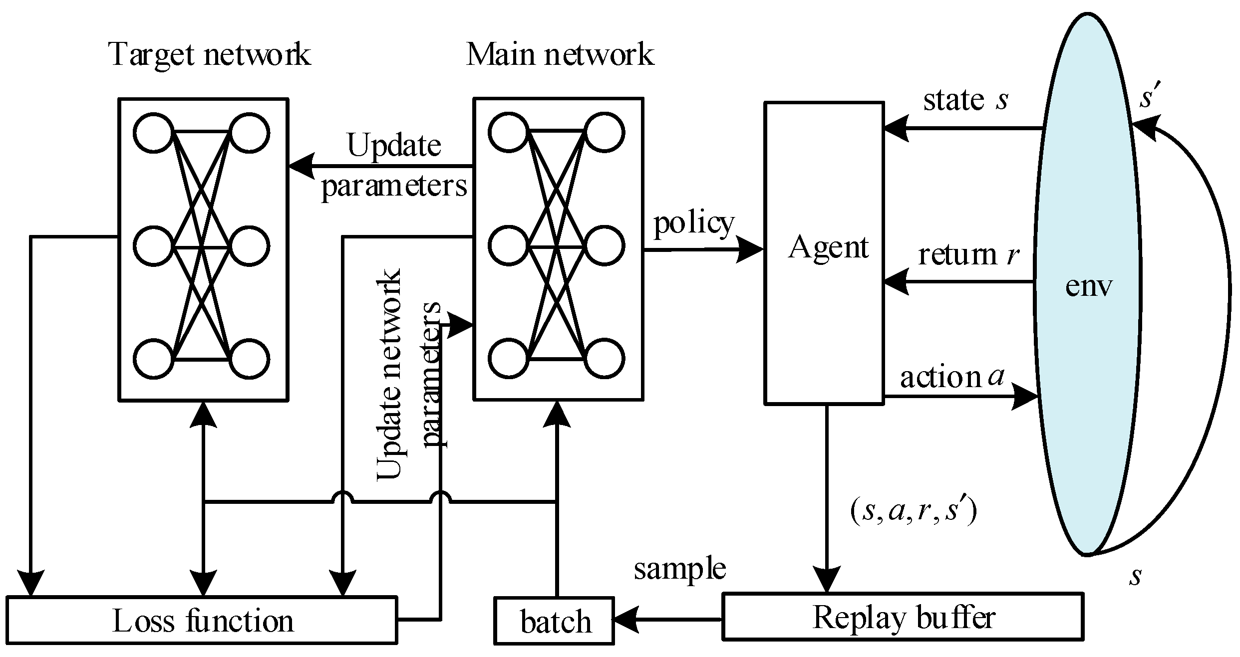
3.1. Reinforcement Learning via Value Function

The RL is about an agent interacting with the environment, learning an optimal policy, by trial and error, for sequential decision making problems [23]. The RL algorithms mainly include RL algorithms based on value function and direct policy search. In RL via value function we evaluates the value function and uses value function to improve the policy, e.g., Q-learning, DQN et al. A value function is a prediction of the expected accumulative discounted future reward, measuring how good each state or state-action pair is [23]. MDPs have become the standard formalism for learning sequential decision making [24]. The goal of RL is to find the optimal strategy for a given MDP [18].

The standard MDPs is defined as $\langle S,A,R,T,\gamma \rangle$, where $S$ is the state set, $A$ is the action set, $R$ is the return function, $T$ is the transfer function, and $\gamma$ is the discount factor. When agent is in state $s\in S$, it takes action $a\in A$ to reach the new state $s^{\prime }\in S$, and gets the return $r=R(s,a)$. The state transition function $T=P(s^{\prime }|s,a)$. Since we are using a model-free MDPs, the transfer function is unknown. State value function $v_{\pi }(s)$ is an estimate of future reward in state $s$ based on strategy $\pi$.

$$v_{\pi }(s)={\displaystyle \sum _a\pi (a/s){\displaystyle \sum _{s^{\prime },r}p(s^{\prime },r/s,a)[r+\gamma v_{\pi }(s^{\prime })]}}$$

(1)

State-action value function $Q_{\pi }(s,a)$ is an estimate of future returns when action $a$ is taken in the state $s$ based on policy $\pi$.

$$Q_{\pi }(s,a)={\displaystyle \sum _{s^{\prime },r}p(s^{\prime },r/s,a)[r+\gamma v_{\pi }(s^{\prime })]}$$

(2)

The optimal $Q^{\ast }(s,a)$ is determined by solving the Bellman equation,

$$Q^{\ast }(s,a)=\mathrm{E}[r+\gamma {\displaystyle \sum _{s^{\prime }}P\left(s^{\prime }|s,a\right)\underset{a^{\prime }}{\max }{Q}^{\ast }(s^{\prime },a^{\prime })}]$$

(3)

The State value function $v_{\pi }(s)$ and the State-action value function $Q_{\pi }(s,a)$ are collectively called value function.

In recent years, DQN [2] is a breakthrough in RL via value function, which extends state space from finite discrete space to infinite continuous space by combining deep neural network with Q-learning [17] algorithm. The principle of DQN is shown in Figure 1.

The data $(s,a,r,s^{\prime })$ generated by the interaction between agent and environment are stored in the replay buffer, which is randomly extracted and provided to the main network and target network. The policy realized evolution through minimizing the Loss function and updating the main network parameters by gradient descent method. The parameters of the target network are updated by copying the main network parameters, after a certain interval. The loss function of DQN is

$$L=[{(r+\gamma \underset{a^{\prime }\in A}{\max }(Q_{\mathrm{target}}(s^{\prime },a^{\prime }))-Q_{\mathrm{main}}(s,a))}^2].$$

(4)

where $r+\gamma \underset{a^{\prime }\in A}{\max }(Q_{\mathrm{target}}(s^{\prime },a^{\prime }))$ is generated by the target network, and $Q_{\mathrm{main}}(s,a)$ is generated by the main network.

The DQN algorithm sets experience replay mechanism [25] and target network with updating parameters asynchronously to break the correlation during training data and then guarantee the stability of the neural network.

Hado et al. proposed the Double-DQN algorithm (DDQN) to solve the problem of overestimation in the DQN algorithm [19]. DDQN does not directly select the max $Q$ value in the target network but uses the corresponding action of the max $Q$ value in the main network to determine the target $Q$ value in the target network. The Loss function of DDQN is

$$L=\mathrm{E}[{(r+\gamma Q_{\mathrm{target}}(s^{\prime },\arg {\max }_{a^{\prime }}(Q_{\mathrm{main}}(s^{\prime },a^{\prime })))-Q_{\mathrm{main}}(s,a))}^2].$$

(5)

DQN and DDQN are the most representative RL algorithms via value function, which are also the benchmarks in our paper.

3.2. Supervised Learning

The goal of SL is to build a concise model of the distribution of class labels in terms of predictor features [26]. In this paper, the agent has been motivated to make favourable decisions in the states with certain characteristics, by using the classification technology in the SL. The demonstrations database for SL consists of $(s,a)$, where $s$ represents state and $a$ represents action. In this paper, cross entropy is used as losses for SL.

4. Our Method

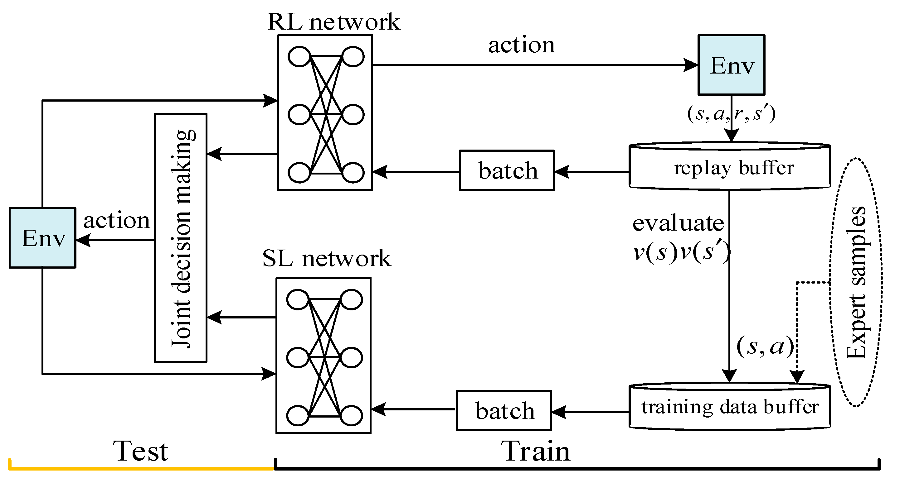
4.1. Supervised Reinforcement Learning via Value Function

SRLVF is mainly based on SL network and RL network, and constructs corresponding training database. The demonstrations can improve the decision-making performance of RL algorithms through SL network.

By introducing decision evaluation mechanism, SRLVF constructs demonstration sets based on the data generated during the interaction between agent and environment, which greatly reduces the dependence on expert samples.

Figure 2 is the framework of our SRLVF approach. In the training phase, the data $(s,a,r,s^{\prime })$ generated by the interaction between the agent and the environment are stored in the experience replay buffer, and batch data are randomly selected from it to train the RL network. The decision-making evaluation mechanism is used to select the superior decision from the experience replay buffer as the demonstrations. The SL network is trained by randomly extracting data from the training data buffer. In the testing phase, the RL network and the SL network jointly make decisions according to different weights. The pseudo-code is shown in Appendix A.

The SRLVF method proposed in this paper is less dependent on expert samples. When expert samples are available, the method can combine expert samples with RL to improve agent decision performance. When the expert samples are very poor or even unavailable, the method can still use the data generated by the interaction between agent and environment to optimize agent’s decision. The purpose of RL is to optimize the overall strategy of the task. There is no evaluation and correction mechanism for decision-making under specific states. SL can fit the mapping model of states and agent actions in expert samples very well. By introducing SL, we can use expert samples to optimize agent’s specific action decision driven by RL, and then realize the combination of expert samples and RL. In the case that the expert samples are difficult to guarantee, we select better state-action pairs from the data generated by the interaction between agent and environment through decision evaluation mechanism and optimize the decision-making under specific states through SL. Most of the current algorithms focus on how to combine expert samples with RL, but less on the objective reality that it is difficult to guarantee the availability of expert samples in different scenarios. The dependence on expert samples greatly limits the application scenarios of the algorithm. Hester et al. proposed a DQfD algorithm for scenarios with only a few expert samples to reduce the dependence on expert samples. Compared with DQfD, the SRLVF method relies less on expert samples and has better applicability to scenarios with different availability of expert samples.

4.2. Demonstration Sets for the SL Network

The process of constructing SL network training data buffer mainly includes the evaluation and storage of data. In state $s$, agents take action $a$, which makes the environment become state $s^{\prime }$. $v(s)$ is an estimate of future reward in state $s$, if $v(s^{\prime })>v(s)$, we can believe that $a$ is a better decision in state $s$, and then store $(s,a)$ in training data buffer. There are three different ways to calculate $v(s)$ in this paper. The first is

$$v_{sum}=v_{\pi }(s)={\displaystyle \sum _{a\in A}\pi (a/s)Q_{\pi }(s,a)},$$

(6)

where $q_{\pi }(s,a)$ is the value function of action $a$ in state $s$. The second is

$$v_{max}=v_{\pi }(s)=\underset{a\in A}{\max }(Q_{\pi }(s,a)),$$

(7)

The third is

$$v_{adaption}=v_{\pi }(s)=(1-\epsilon )\ast \underset{a\in A}{\max }(q_{\pi }(s,a))+\epsilon \ast \frac{\underset{a\in (A-a_{\max })}{sum}(q_{\pi }(s,a))}{n-1}.$$

(8)

where $\epsilon$ is the exploratory ability of RL to adopt $\epsilon -greedy$ strategy in the training process, $v_{adaption}$ adds an adaptive adjustment based on exploratory probability $\epsilon$, which makes the calculation of state value function $v(s)$ more objective. $v_{sum}$, $v_{max}$ and $v_{adaption}$ are obtained on the basis of Equations (1) and (2) taking into account the influence of different factors. The difference between $v_{sum}$ and $v_{adaption}$ is that the probability used to compute $v_{sum}$ is obtained through softmax function, but when computing $v_{adaption}$ the probability is defined by the $\epsilon -greedy$ policy. $v_{max}$ and $v_{adaption}$ are identical when $\epsilon =0$. In SRLVF method, the state value function is the criterion of selecting demonstrations, so the way of calculating the state value function affects the quality of demonstrations, $v_{adaption}$ is the most accurate computing mode, but $\epsilon$ gradually decreases with the training process, and the criterion for selecting demonstrations eventually becomes $v_{max}$. Because the state value function and the state-action value function are both estimates of the future total return under the current strategy rather than accurate values, in order to obtain the optimal selection criteria, we will simulate and validate the performance of three calculation models of the value function in the experimental part.

The introduction of decision evaluation mechanism has expanded the source of demonstrations and formed a powerful supplement to the expert samples, which can effectively reduce the dependence on expert samples.

4.3. Generalization of SRLVF

In the SRLVF method, the demonstrations are selected from the data generated by the interaction between agent and environment driven by RL algorithms through decision-making evaluation mechanism and then optimizes the performance of RL algorithm by using the demonstrations and existing expert data through SL. In SRLVF method, the data which can optimize decision-making include the demonstrations generated by the interaction between agent and environment and the existing expert samples in different application scenarios.

It is difficult to guarantee the availability of expert samples in different scenarios. When expert samples can’t play a role in decision-making optimization or even have poor availability, effective data mainly comes from the interaction between agent and environment. These data optimize decision-making through the SL network, so there is no generalization problem for SL network. At this time, the generalization of SRLVF is mainly influenced by RL algorithms. However, the performance of different RL algorithms in different scenarios is different.

When the quality and quantity of expert samples can be guaranteed, the performance of SRLVF method is affected by expert samples. The expert samples optimize the decision-making of RL algorithms through the SL network, which has a beneficial impact on the generalization performance of SRLVF method.

5. Experiments

For sequential decision-making tasks modelled by MDPs, each individual task instance needs a sequence of decisions to bring the agent from a starting state to a goal state. According to the length of the decision-making sequence from a starting state to a target state, decision tasks can be divided into three categories: finite, fixed horizon tasks, indefinite horizon tasks, and infinite horizon tasks. In finite, fixed horizon tasks the length of the decision-making sequence is fixed. In indefinite horizon tasks, the decision-making sequence can have arbitrary length and end at the goal state. In the infinite horizon tasks, the decision-making sequence does not end in the goal state. The application conditions of the first model are strict and so its scope of application is limited, for example tutoring students for exams or handling customer service requests. The other two types of tasks are the focus of our attention. In Puckworld scenario, the decision-making process will end in the goal state and the length of the decision-making sequence is not fixed, so Puckworld is the type of indefinite horizon tasks. In Pendulum scenario, the decision-making process can’t end to keep the agent in the goal state, so the Pendulum belongs to the kind of infinite horizon tasks. The Puckworld and Pendulum scenarios represent two types of sequential decision-making tasks modelled by MDPs. So we choose these two scenarios as our agent environment.

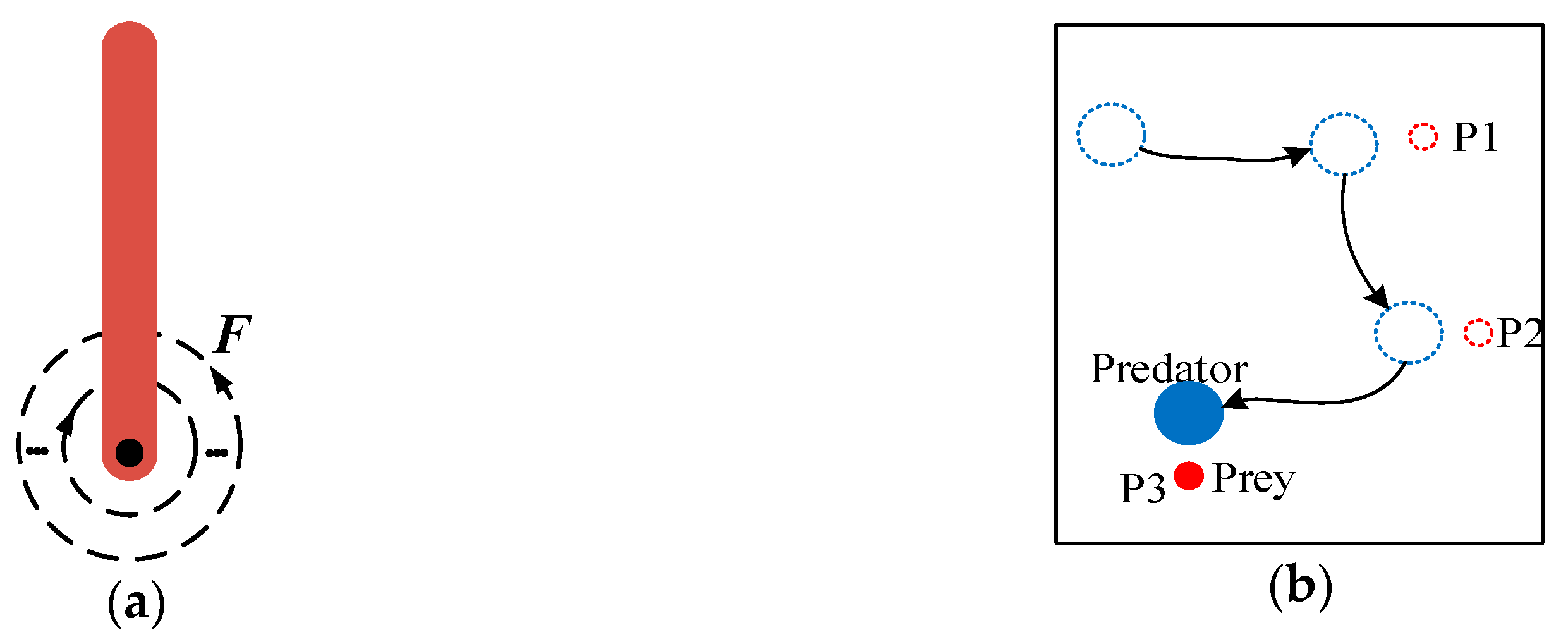
5.1. Experimental Setup

In both Pendulum and Puckworld scenarios, the performance of SRLVF method is verified. The (a) of Figure 3 is the Pendulum scenarios, which is an experimental scenario of RL algorithm provided by gym. In this scenario, the pendulum is ensured to be inverted by continuously applying force $F_c$ in different directions and sizes. In order to adapt to the application characteristics of the RL algorithm based on value function, the continuous force $F_c\in [-2,2]$ in the original scenario is discretized into $F_d\in [0,\pm 0.4,\pm 0.8,\pm 1.2,\pm 1.6,\pm 2.0]$.

The Puckworld scenarios is the (b) of Figure 3 with reference to the code written by Qiang Ye [27]. In Puckworld scenarios, it mainly includes a predator and a prey. Predator can move freely in four directions. Prey’s position changes randomly in a fixed time interval. Predator captures Prey as an agent.

Algorithm and Hyperparameter

SRLVF combines RL with demonstrations through SL. In the experiment, we use DQN and DDQN as benchmark algorithms to verify the effectiveness of SRLVF method. The RL part of SRLVF method adopts DQN algorithm and DDQN algorithm, which we call SRLVF-based DQN (SDQN) and SRLVF-based DDQN (SDDQN) respectively. The SL part of SRLVF method uses demonstrations to train the neural network.

The principles of DQN and DDQN have been analyzed in Section 3.2. Both DQN and DDQN have two neural networks: the main network and the target network. Both the two networks are set up as two layers fully connected networks with 25 units per layer. In the RL network, the discount factor $\gamma$ is 0.9 and the learning rate $l$ is 0.005. The SL network is a 2 fully connected network with 128 units per layer. In the SL network, the learning rate $l$ is 0.01, the loss function was computed by cross-entropy.

5.2. Result and Analysis

In order to evaluate the performance of SRLVF, we tested the performance of SDQN and SDDQN in Pendulum and Puckworld scenarios, as well as the influence of different computing modes of $v(s)$. The code is implemented based on python 3.5 with Tensorflow 1.12.0 and Gym 0.10.9. As illustrated in Figure 4, Figure 5 and Figure 6, each averaged reward curve is computed 7 times with a continuous error bar.

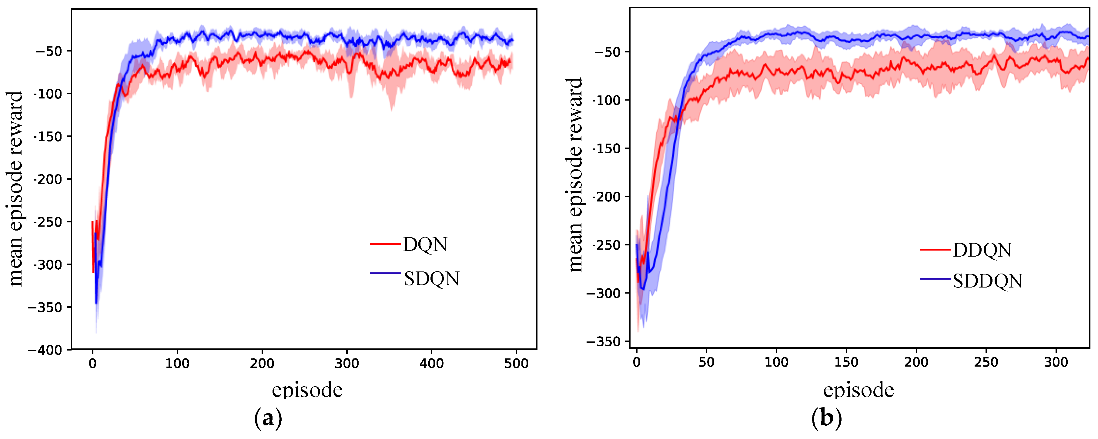
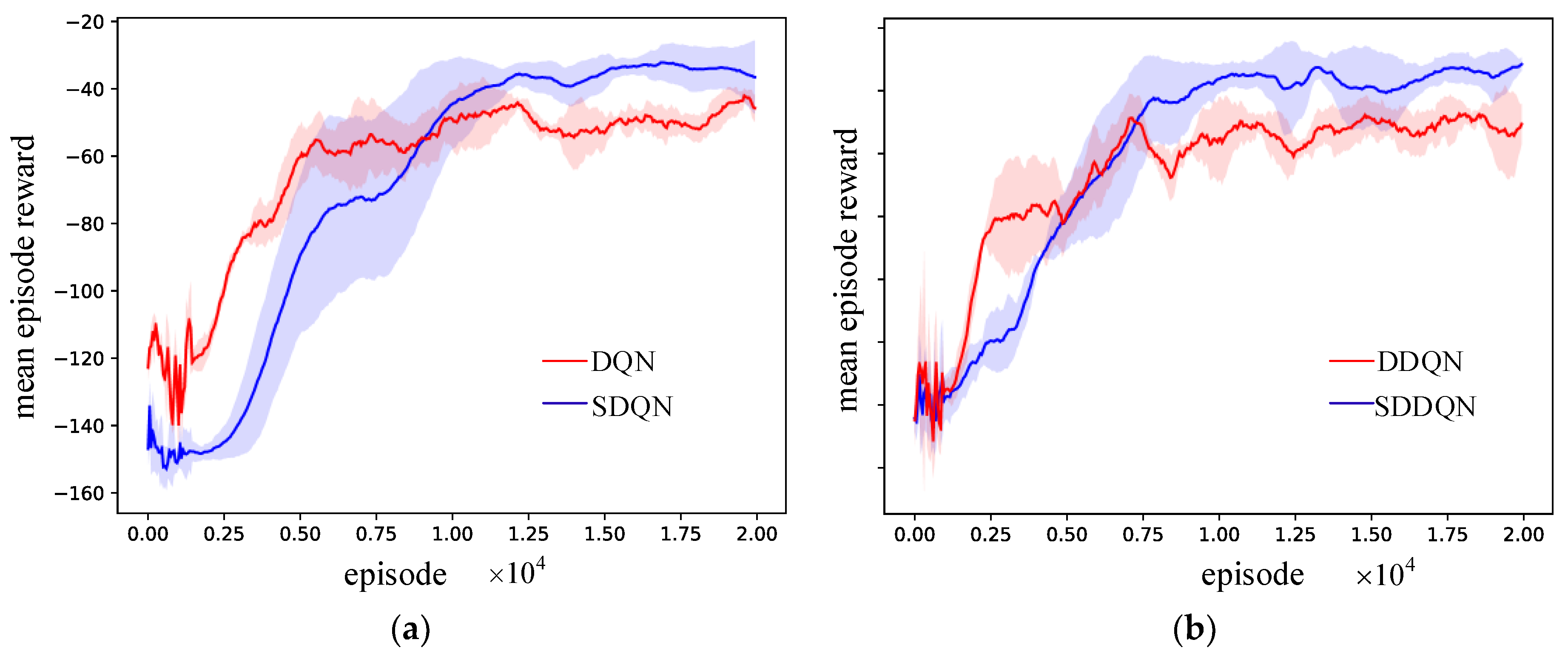
5.2.1. Testing the Performance of the SRLVF Method

Figure 4 and Figure 5 show that SDQN and SDDQN are better than DQN and DDQN respectively in both Pendulum and Puckworld scenarios, but both of them have worse performance before convergence.

Our algorithm outperforms the benchmark algorithm after convergence. We know that the purpose of RL is to approximate the overall strategy, while the decision-making under specific states is unstable. However, SL can optimize the decision making performance by training with demonstrations. SRLVF can improve the overall performance of the algorithm by combing RL with SL.

In SRLVF method, we use demonstrations to optimize the decision-making of RL algorithms through SL network in order to improve the performance. Differ from the convergence process of RL algorithms only involves the training of RL network, the convergence process of SRLVF method includes the training of RL network and SL network. Because the demonstrations for training SL network come from the interaction between agent and environment driven by the RL algorithm, and the institutional characteristics of demonstrations are also changing in the process of training RL network, the convergence of the SL network lags behind that of the RL network. In the convergence process of the SRLVF method, the SL network can’t optimize the performance of the RL algorithm because it has not yet converged, and even has adverse effects. So in the convergence stage, the performance of SRLVF method is worse than benchmark algorithm.

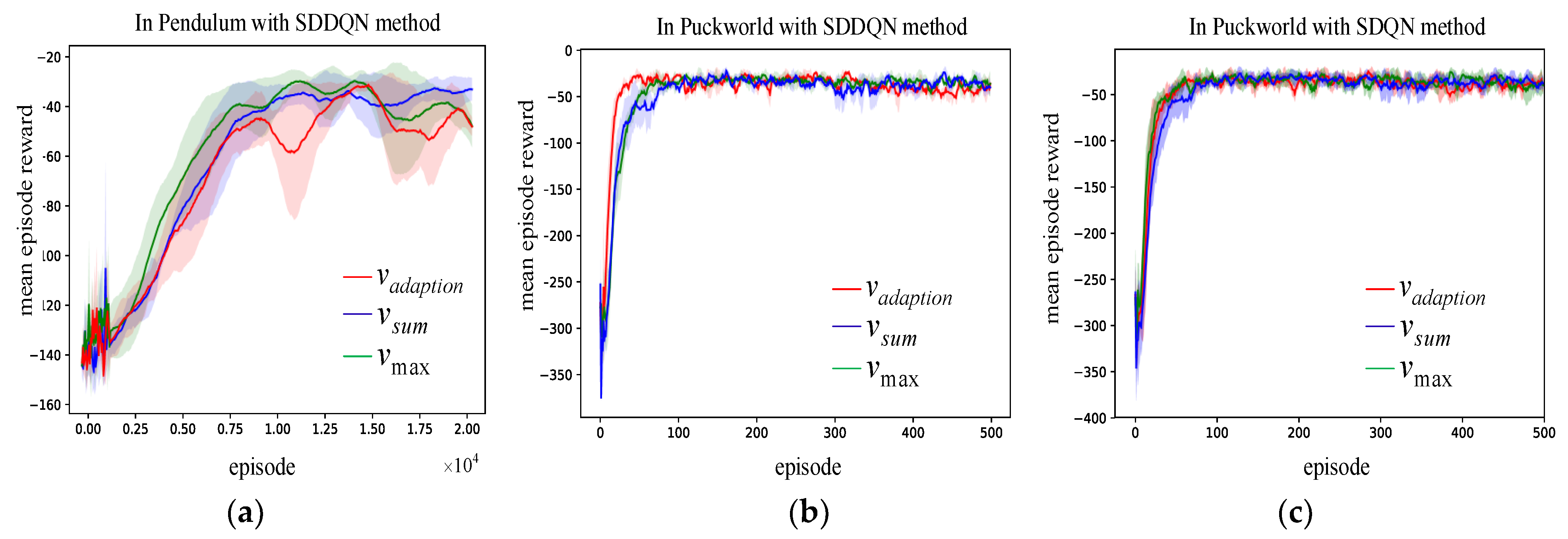
5.2.2. Evaluating the Impact of Different $v(s)$ Calculation Methods on the Performance of SRLVF

In Pendulum and Puckworld scenarios, we test the performance of SDQN and SDDQN algorithms Which use three computational methods: $v_{max}$, $v_{adaption}$ and $v_{sum}$ respectively.

As shown in the Figure 6, the performance of SDQN and SDDQN algorithms with different $v(s)$ computing methods does not differ greatly in both Pendulum and Puckworld scenarios, especially in Puckworld scenario, the performance of the algorithms is much the same. In Pendulum scenario, the performance of SDDQN with $v_{adaption}$ is slightly worse, but it is the best in Puckworld scenarios. The performance of SDQN with $v_{adaption}$ is not the best in Puckworld scenarios. These results show that the impact of different $v(s)$ on SRLVF performance is related to RL algorithm and scenarios, so the $v(s)$ computing method needs to be selected according to the specific situation.

Value function is an estimated value rather than a deterministic value. In our method, the value function is approximated by the neural network, which is affected by many factors, such as network parameters, reward functions, reward delay length, the task characteristics, et al. We can indeed select the high quality demonstrations to improve the performance through using the state value function obtained by three calculation methods as the selection criterion of demonstrations. However, there are many factors affecting the estimation of the value function, it is difficult to get the selection rules of the three calculation models.

6. Conclusions and Future Work

Based on experimental results we claim that even if expert samples are not available, the SRLVF method presented in this work still improves the performance of the RL via value function algorithm. The method presented in this work greatly reduces the requirement for the availability of expert samples. Combining RL algorithms with expert samples brings a number of issues which are worth addressing. SRLVF method is designed for the objective condition that the availability of expert samples is difficult to guarantee in different scenarios. In our view, there are two interesting research directions: (1) improving the performance of SRLVF in the stage of training through a few expert samples by expanding the combination style of expert samples and RL. (2) Estimating the state function more accurately and provide more accurate criteria for choosing demonstrations.

References

1. Mnih, V.; Kavukcuoglu, K.; Silver, D.; Graves, A.; Antonoglou, I.; Wierstra, D.; Riedmiller, M. Playing atari with deep reinforcement learning. Available online: https://arxiv.org/pdf/1312.5602 (accessed on 15 March 2019).
2. Mnih, V.; Kavukcuoglu, K.; Silver, D.; Rusu, A.A.; Veness, J.; Bellemare, M.G.; Graves, A.; Riedmiller, M.; Fidjeland, A.K.; Ostrovski, G. Human-level control through deep reinforcement learning. Nature 2015, 518, 529. [Google Scholar] [CrossRef] [PubMed]
3. Silver, D.; Schrittwieser, J.; Simonyan, K.; Antonoglou, I.; Huang, A.; Guez, A.; Hubert, T.; Baker, L.; Lai, M.; Bolton, A. Mastering the game of go without human knowledge. Nature 2017, 550, 354. [Google Scholar] [CrossRef] [PubMed]
4. Silver, D.; Huang, A.; Maddison, C.J.; Guez, A.; Sifre, L.; Van Den Driessche, G.; Schrittwieser, J.; Antonoglou, I.; Panneershelvam, V.; Lanctot, M. Mastering the game of Go with deep neural networks and tree search. Nature 2016, 529, 484. [Google Scholar] [CrossRef] [PubMed]
5. Levine, S.; Finn, C.; Darrell, T.; Abbeel, P. End-to-end training of deep visuomotor policies. J. Mach. Learn. Res. 2016, 17, 1334–1373. [Google Scholar]
6. Oh, J.; Guo, X.; Lee, H.; Lewis, R.L.; Singh, S. Action-conditional video prediction using deep networks in atari games. In Proceedings of the Advances in Neural Information Processing Systems, Montreal, ON, Canada, 7–12 December 2015; pp. 2863–2871. [Google Scholar]
7. Zhu, Y.; Mottaghi, R.; Kolve, E.; Lim, J.J.; Gupta, A.; Fei-Fei, L.; Farhadi, A. Target-driven visual navigation in indoor scenes using deep reinforcement learning. In Proceedings of the 2017 IEEE International Conference on Robotics and Automation (ICRA), Singapore, 29 May–3 June 2017. [Google Scholar]
8. Tesauro, G.; Das, R.; Chan, H.; Kephart, J.; Levine, D.; Rawson, F.; Lefurgy, C. Managing power consumption and performance of computing systems using reinforcement learning. In Proceedings of the Advances in Neural Information Processing Systems, Vancouver, BC, Canada, 8–10 December 2008. [Google Scholar]
9. Zoph, B.; Le, Q.V. Neural architecture search with reinforcement learning. Available online: https://arxiv.org/pdf/1611.01578 (accessed on 15 March 2019).
10. Duan, Y.; Schulman, J.; Chen, X.; Bartlett, P.L.; Sutskever, I.; Abbeel, P. RL2: Fast Reinforcement Learning via Slow Reinforcement Learning. Available online: https://arxiv.org/pdf/1611.02779 (accessed on 15 March 2019).
11. Nair, A.; McGrew, B.; Andrychowicz, M.; Zaremba, W.; Abbeel, P. Overcoming exploration in reinforcement learning with demonstrations. Available online: https://arxiv.org/pdf/1709.10089 (accessed on 15 March 2019).
12. Lakshminarayanan, A.S.; Ozair, S.; Bengio, Y. Reinforcement learning with few expert demonstrations. In Proceedings of the NIPS Workshop on Deep Learning for Action and Interaction, Barcelona, Spain, 10 December 2016. [Google Scholar]
13. Zhang, X.; Ma, H. Pretraining deep actor-critic reinforcement learning algorithms with expert demonstrations. Available online: https://arxiv.org/pdf/1801.10459 (accessed on 15 March 2019).
14. Hester, T.; Vecerik, M.; Pietquin, O.; Lanctot, M.; Schaul, T.; Piot, B.; Horgan, D.; Quan, J.; Sendonaris, A.; Osband, I. Deep q-learning from demonstrations. In Proceedings of the Thirty-Second AAAI Conference on Artificial Intelligence, New Orleans, LA, USA, 2–7 February 2018. [Google Scholar]
15. Cruz, G.V., Jr.; Du, Y.; Taylor, M.E. Pre-training neural networks with human demonstrations for deep reinforcement learning. Available online: https://arxiv.org/pdf/1709.04083 (accessed on 15 March 2019).
16. Rajeswaran, A.; Kumar, V.; Gupta, A.; Vezzani, G.; Schulman, J.; Todorov, E.; Levine, S. Learning complex dexterous manipulation with deep reinforcement learning and demonstrations. Available online: https://arxiv.org/pdf/1709.10087 (accessed on 15 March 2019).
17. Watkins, C.J.C.H.; Dayan, P. Q-learning. Mach. Learn. 1992, 8, 279–292. [Google Scholar] [CrossRef] [Green Version]
18. Sutton, R.S.; Barto, A.G. Reinforcement Learning: An Introduction; Springer Science & Business Media: Berlin, Germany, 1992. [Google Scholar]
19. Van Hasselt, H.; Guez, A.; Silver, D. Deep reinforcement learning with double q-learning. In Proceedings of the Thirtieth AAAI Conference on Artificial Intelligence, Phoenix, AZ, USA, 12–17 February 2016. [Google Scholar]
20. Wang, Z.; Schaul, T.; Hessel, M.; Van Hasselt, H.; Lanctot, M.; De Freitas, N. Dueling network architectures for deep reinforcement learning. Available online: https://arxiv.org/pdf/1511.06581 (accessed on 15 March 2019).
21. Mnih, V.; Badia, A.P.; Mirza, M.; Graves, A.; Lillicrap, T.; Harley, T.; Silver, D.; Kavukcuoglu, K. Asynchronous methods for deep reinforcement learning. In Proceedings of the International Conference on Machine Learning, New York, NY, USA, 19–24 June 2016. [Google Scholar]
22. Lipton, Z.C.; Gao, J.; Li, L.; Li, X.; Ahmed, F.; Deng, L. Efficient Exploration for Dialog Policy Learning with Deep BBQ Networks & Replay Buffer Spiking. Available online: https://arxiv.org/pdf/1608.05081 (accessed on 15 March 2019).
23. Li, Y. Deep reinforcement learning: An overview. Available online: https://arxiv.org/pdf/1701.07274 (accessed on 15 March 2019).
24. Van Otterlo, M.; Wiering, M. Reinforcement Learning and Markov Decision Processes. Reinforc. Learn. 2012, 12, 3–42. [Google Scholar]
25. Schaul, T.; Quan, J.; Antonoglou, I.; Silver, D. Prioritized Experience Replay. Nature 2015, 518, 529–533. [Google Scholar]
26. Kotsiantis, S.B.; Zaharakis, I.; Pintelas, P. Supervised machine learning: A review of classification techniques. Emerg. Artif. Intell. Appl. Comput. Eng. 2007, 160, 3–24. [Google Scholar]
27. Ye, Q. Reinforce. Available online: https://github.com/qqiang00/reinforce (accessed on 15 March 2019).
Figure 1. The principle of DQN.
Symmetry 11 00590 g001
Figure 2. The framework of SRLVF.
Symmetry 11 00590 g002
Figure 3. Pendulum (a) and Puckworld (b).
Symmetry 11 00590 g003
Figure 4. (a) Average rewards on DQN and SDQN in Puckworld. (b) Average rewards on DDQN and SDDQN in Puckworld too.
Symmetry 11 00590 g004
Figure 5. (a) Average rewards on DQN and SDQN in Pendulum. (b) Average rewards on DDQN and SDDQN in Pendulum too.
Symmetry 11 00590 g005
Figure 6. (a) Average rewards on SDDQN using different v ( s ) in Pendulum. (b) Average rewards on SDDQN using different v ( s ) in Puckworld. (c) Average rewards on SDQN using different v ( s ) in Puckworld too.
Symmetry 11 00590 g006