Article

Tracking Control of a Class of Chaotic Systems

1
School of Mathematics and Statistics, Qilu University of Technology (Shandong Academy of Science), Jinan 250353, China
2
School of Electrical Engineering and Automation, Qilu University of Technology (Shandong Academy of Science), Jinan 250353, China
*
Author to whom correspondence should be addressed.
Symmetry 2019, 11(4), 568; https://doi.org/10.3390/sym11040568
Submission received: 20 February 2019 / Revised: 21 March 2019 / Accepted: 12 April 2019 / Published: 19 April 2019

Abstract

:
This paper investigates the asymptotic tracking control problem of the chaotic system. Firstly, a reference system is presented, the output of which can asymptotically track a given command. Then, a both physically implementable and simple controller is designed, by which the given chaotic system synchronizes the reference system, and thus the output of such chaotic systems can asymptotically track the given command. It should be pointed out that the output of the given chaotic system can asymptotically track arbitrary desired periodic orbits. Finally, several illustrative examples are taken as example to show the validity and effectiveness of the obtained results.

1. Introduction

Since Lorenz firstly found the chaos phenomenon when investigating the atmosphere in 1963, both chaotic systems and chaotic dynamics have been investigated extensively in many kinds of fields, e.g., physics, engineering, biology, ecology, economics, and even in some fields of the social sciences. In 1990, chaos control was firstly proposed by Ott, Grebogi and York, and this method is called the OGY method [1]. Meanwhile, the PC method [2] for chaos synchronization (i.e., complete synchronization) was firstly presented by Pecora and Carroll. Up to date, many types of chaos synchronization have been proposed, see Refs. [2,3,4,5,6,7,8,9,10,11,12,13,14,15]. However, for the chaotic systems, there still are many both interesting and valuable questions that need to be investigated further.
It is well known that the asymptotic tracking control problem of the chaotic systems is very important in both theorem and applications. However, for such a problem there exist some important things which should be considered. On the one hand, in most of the existing results, it should be pointed out that the asymptotic tracking performance cannot be achieved. In fact, instead of asymptotic tracking performance, only the so-called bounded-error trajectory tracking was ensured, see Refs. [16,17,18]. On the other hand, the aim of most of the tracking control methods is to force the states of a given arbitrary dimensional chaotic system to its equilibrium point, e.g., origin. In this case, the given chaotic system is stabilized. Although some approaches can track arbitrary desired trajectories, most of them only force one state of a given system to an arbitrary desired trajectory [19,20,21]. As far as we know, there are very few published papers about driving some states of a given chaotic system to arbitrary desired periodic orbits, and the designed controllers are too complicated to be utilized in applications. Therefore, driving some states of a chaotic system to arbitrary desired trajectories has not been fully completed yet, which motivates our present work.
This paper investigates the asymptotic tracking control of the chaotic systems. A reference system is firstly presented, the output of which can asymptotically track a given command. A physically implementable controller is then designed to guarantee the given chaotic system synchronizes the reference system, and thus the output of such chaotic systems can asymptotically track the given command.

2. Problem Formation

Consider the following n-dimensional autonomous chaotic system:
w ˙ = F ( w )
where w ˙ stands for the derivative of w about time t, w R n is the state and F ( w ) R n is a continuous vector function.
For the system (1), the corresponding controlled system is given as:
w ˙ = F ( w ) + U y = G w
where U R n is the controller to be designed, y R p is the output of the system (2) and C R p × n , p 1 .
For the system (2), we can make a non-singular transform: v = T w which can transfer the system (2) into the following system:
x ˙ = A ( z ) x + B u z ˙ = f ( x , z ) y = C x
where v = ( x , z ) R n is the state, x R m , z R n m , m 2 , A ( z ) R m × m , f ( x , z ) R n m is a continuous function vector, B R m × q is the control matrix having full column rank, q 1 , ( A ( z ) , B ) is a controllable pair, C R p × m .
Remark 1.
According to the results in [10], for the system (2), the non-singular transform: v = T w is obtained if this system can be controlled completely. In addition, we shall give the procedure of obtaining the matrix T and the vector B to meet the conditions of system (3) in Section 4.
The aim of this paper is to study the asymptotic tracking control problem of the given system (3), i.e., to design a both physically implementable and simple controller u ( t ) to meet the following performance:
lim t y = c ( t )
where c ( t ) is given as
c ( t ) = ( c 1 ( t ) , , c p ( t ) ) T R p , 1 p m
and assumed to be piecewise smooth (or continuous) and uniformly bounded.

3. Main Result

In order to realize the asymptotic tracking control of the given n-dimensional chaotic system (3), a reference system is firstly proposed to asymptotically track the given command, then a both physically implementable and simple controller is designed to guarantee the complete synchronization between the reference system and the given chaotic system. In other words, two steps are provided to solve such a problem. One step is to present a reference system, the other step is to design a both physically implementable and simple controller.

3.1. The Reference Model

The n-dimensional reference chaotic system is designed as follows:
x ˙ r = A ( z ) + B K ( z ) x r + B r ( z ) c ( t ) + D r c ˙ ( t ) z ˙ = f ( x , z ) y r = C x r
where ( x r , z ) R n is the state, x r = ( x r 1 , x r 2 , , x r m ) T R m , m 2 , C is given in (3), c ( t ) is given in (5), K ( z ) is a feedback gain matrix with appropriate dimension, which is chosen to make the matrix A ( z ) B K ( z ) be Hurwitz with two blocks N 1 ( z ) , N 2 ( z ) , i.e.,
A ( z ) + B K ( z ) = ( N 1 ( z ) , N 2 ( z ) ) ,
where N 1 ( z ) R m × p , N 2 ( z ) R m × ( m p ) , B r ( z ) R m × p is a matrix and
D r = I p 0 R m × p ,
I p is the p × p identify matrix.
Remark 2.
For this reference model (6), the feedback gain matrix K ( z ) is designed by the zero pole configuration method in linear system control. In addition, for the system (6), the most general case is B r ( z ) = ( A ( z ) + B K ( z ) ) , D r = I m , where I m is the m × m identify matrix. In this case, x r i ( t ) c i ( t ) , i = 1 , , m , as t . Moreover, if c ( t ) is only a constant command, then set D r = 0 .
The following theorem presents the asymptotically convergence of the reference model (6).
Theorem 1.
Consider the system (6). The state x r can globally asymptotically track any piecewise smooth (or continuous) and uniformly bounded command ( c ( t ) , 0 ) T R m .
Proof. 
Let Y = x r ( c ( t ) , 0 ) T , we obtain that the system Y ˙ = ( A ( z ) + B K ( z ) ) Y is globally asymptotically stable with respect to the origin since the matrix A ( z ) + B K ( z ) is Hurwitz. Thus, Y 0 , i.e., x r ( c ( t ) , 0 ) T , as t . About the system Y ˙ = ( A ( z ) + B K ( z ) ) Y , we can achieve that
x ˙ r c ˙ ( t ) 0 = A ( z ) + B K ( z ) x r c ( t ) 0
i.e.,
x ˙ r = A ( z ) + B K ( z ) x r A ( z ) + B K ( z ) c ( t ) 0 + c ˙ ( t ) 0 .
Further, it results in
x ˙ r = A ( z ) + B K ( z ) x r ( N 1 ( z ) , N 2 ( z ) ) c ( t ) 0 + I p 0 0 I m p c ˙ ( t ) 0 .
After simple computation, it becomes
x ˙ r = A ( z ) + B K ( z ) x r N 1 ( z ) c ( t ) + I p 0 c ˙ ( t )
that is
x ˙ r = A ( z ) + B K ( z ) x r + B r ( z ) c ( t ) + D r c ˙ ( t ) .
This completes the proof. □

3.2. Control Design

In the next, designing a both physically implementable and simple controller u ( t ) for (3) to make x asymptotically track the command ( c ( t ) , 0 ) T is equivalent to designing a both physically implementable and simple controller u ( t ) to make x asymptotically track the reference trajectory x r , i.e., the tracking error e ( t ) = x r x asymptotically converges to zero. The desired error dynamics system is specified as
e ˙ = A ( z ) + B K ( z ) e
where K ( z ) is designed in the reference model (6).
Combining (3), (6), (9), it results in
A ( z ) + B K ( z ) x r + B r c ( t ) + D r c ˙ ( t ) A ( z ) x ( t ) B u ( t ) = A ( z ) + B K ( z ) e
Based on (10), then control signal u ( t ) should satisfy
B u ( t ) = B K ( z ) x ( t ) + B r c ( t ) + D r c ˙ ( t )
The control law is obtained, i.e.,
u ( t ) = B + B K ( z ) x ( t ) + B + B r c ( t ) + D r c ˙ ( t ) = K ( z ) x + B + B r c ( t ) + D r c ˙ ( t )
where B + = ( B T B ) 1 B T is the pseudo-inverse of B.
Remark 3.
About the controller u ( t ) given in (12), three cases are stated as follows:
Case 1: If B 1 exists, then the controller u ( t ) given in (12) is an accurate solution of (11). In this case, the state x of the system (3) asymptotically tracks the state x r of the reference system (6), and x i asymptotically tracks the command c i ( t ) , i = 1 , 2 , , p .
Case 2: If B is not invertible, then the controller u ( t ) given in (12) is an accurate solution of (11) if and only if the following structural constraint
[ I B B + ] B K ( z ) x ( t ) + B r c ( t ) + D r c ˙ ( t ) 0
is satisfied. In this case, the state x of the system (3) asymptotically tracks the state x r of the reference system (6), and x i asymptotically tracks the constant command c i ( t ) , i = 1 , 2 , , p .
Case 3: If both B is not invertible and the structural constraint (13) is not satisfied, then the controller u ( t ) given in (12) is only an approximate solution of (11). In this case, the performance of this controller u ( t ) can be improved by adjusting the feedback gain matrix K.

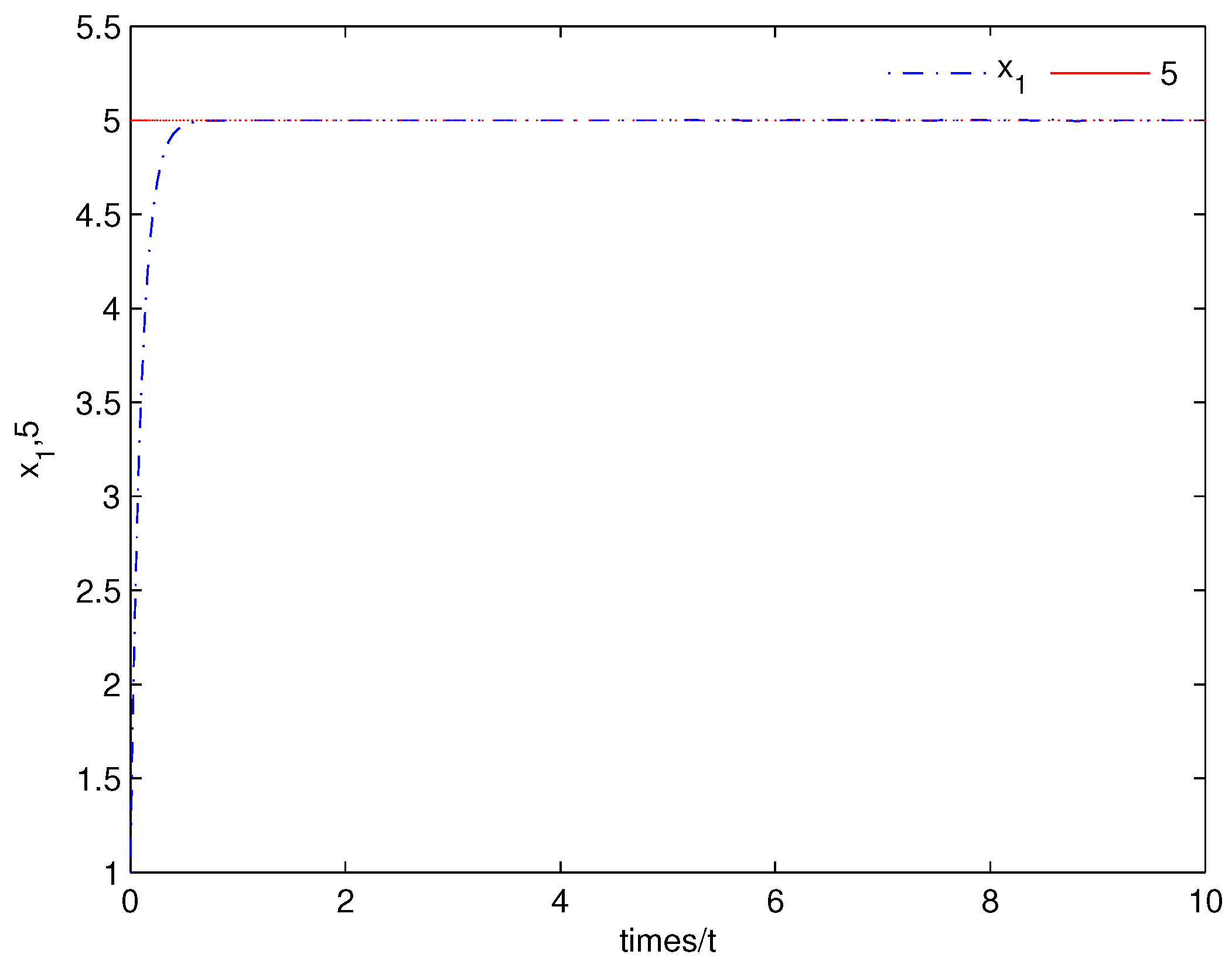
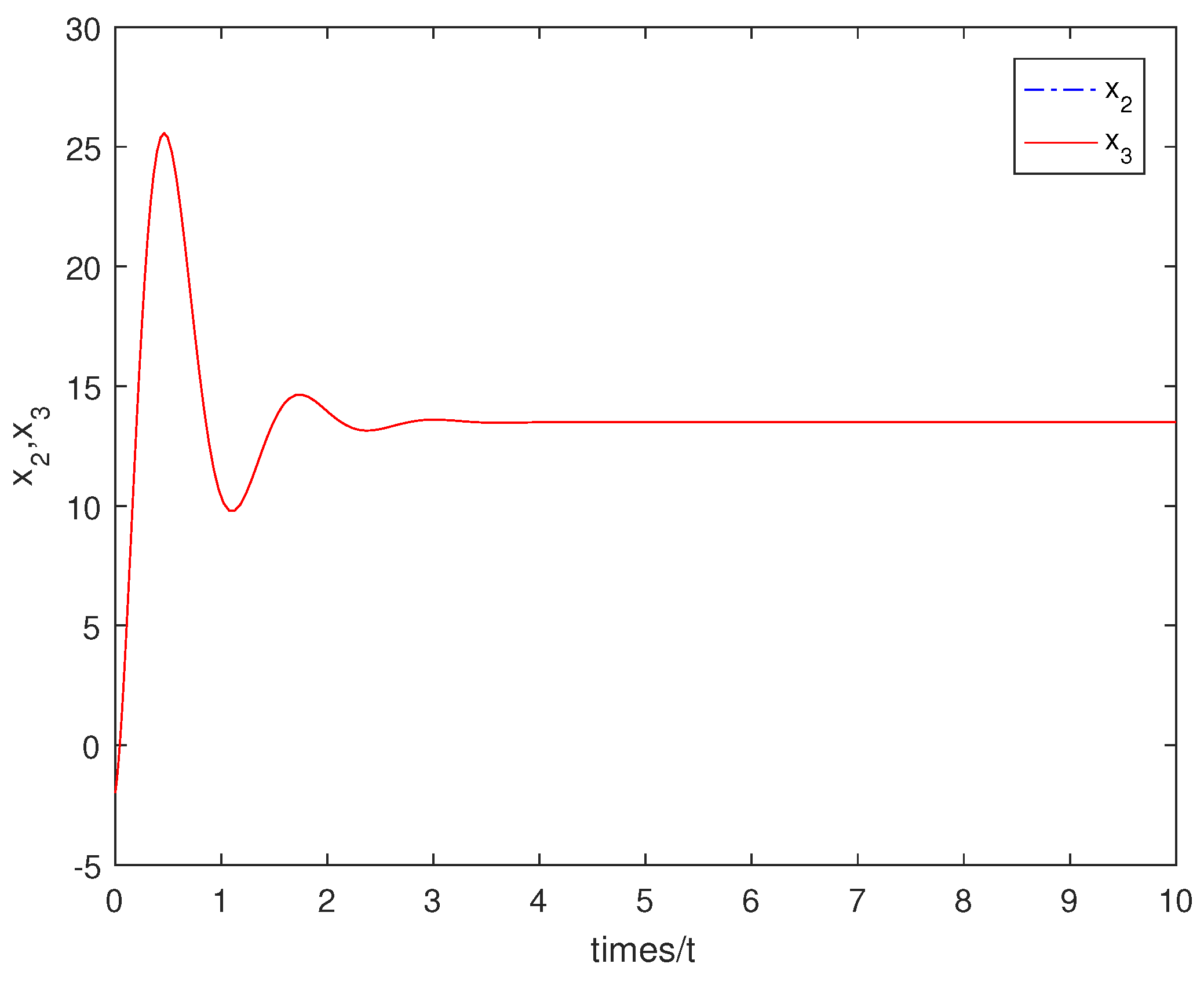
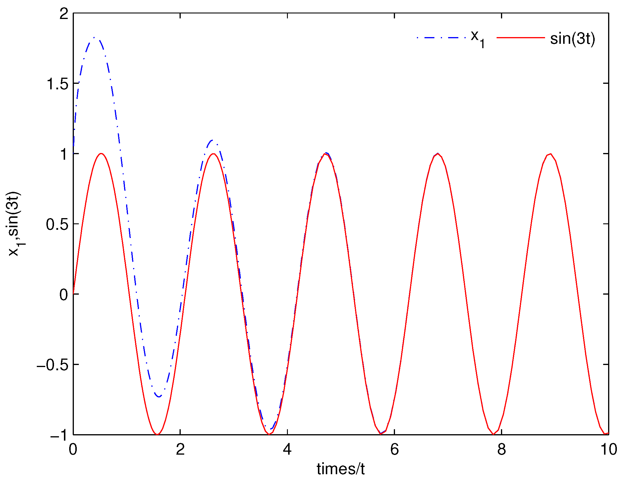
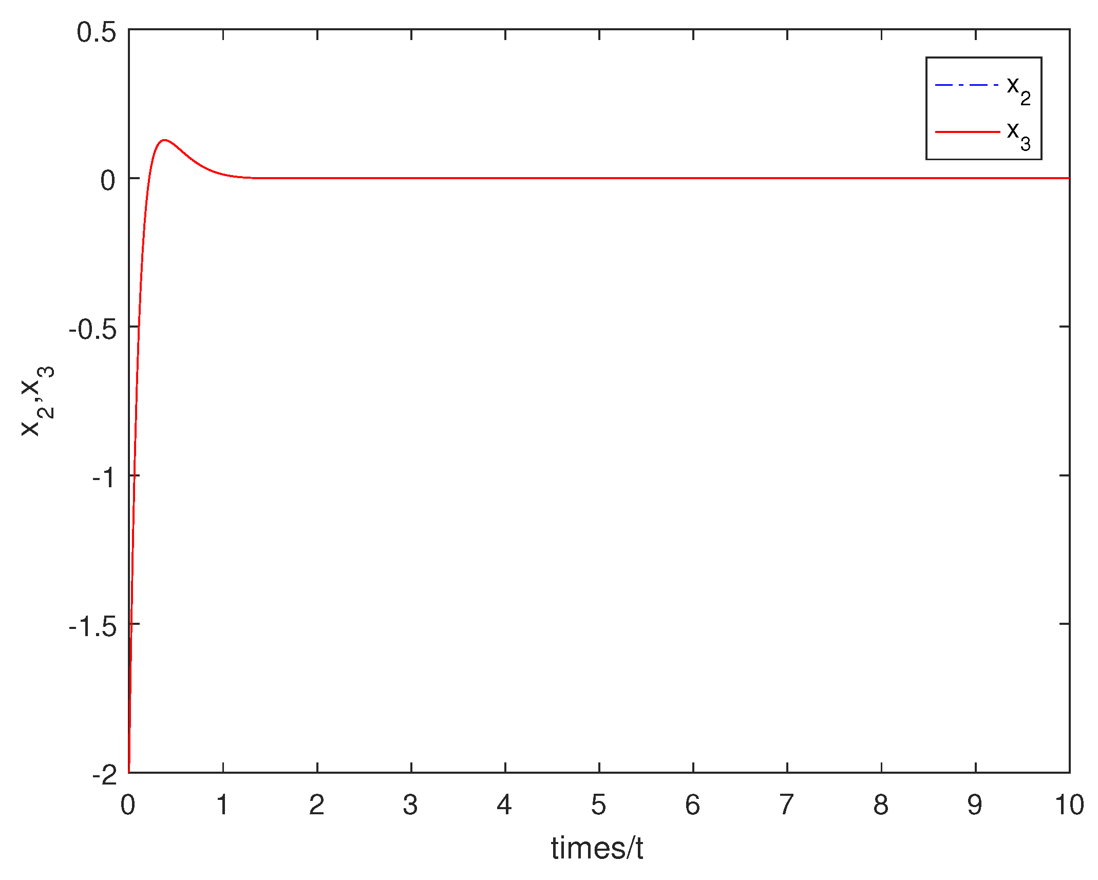
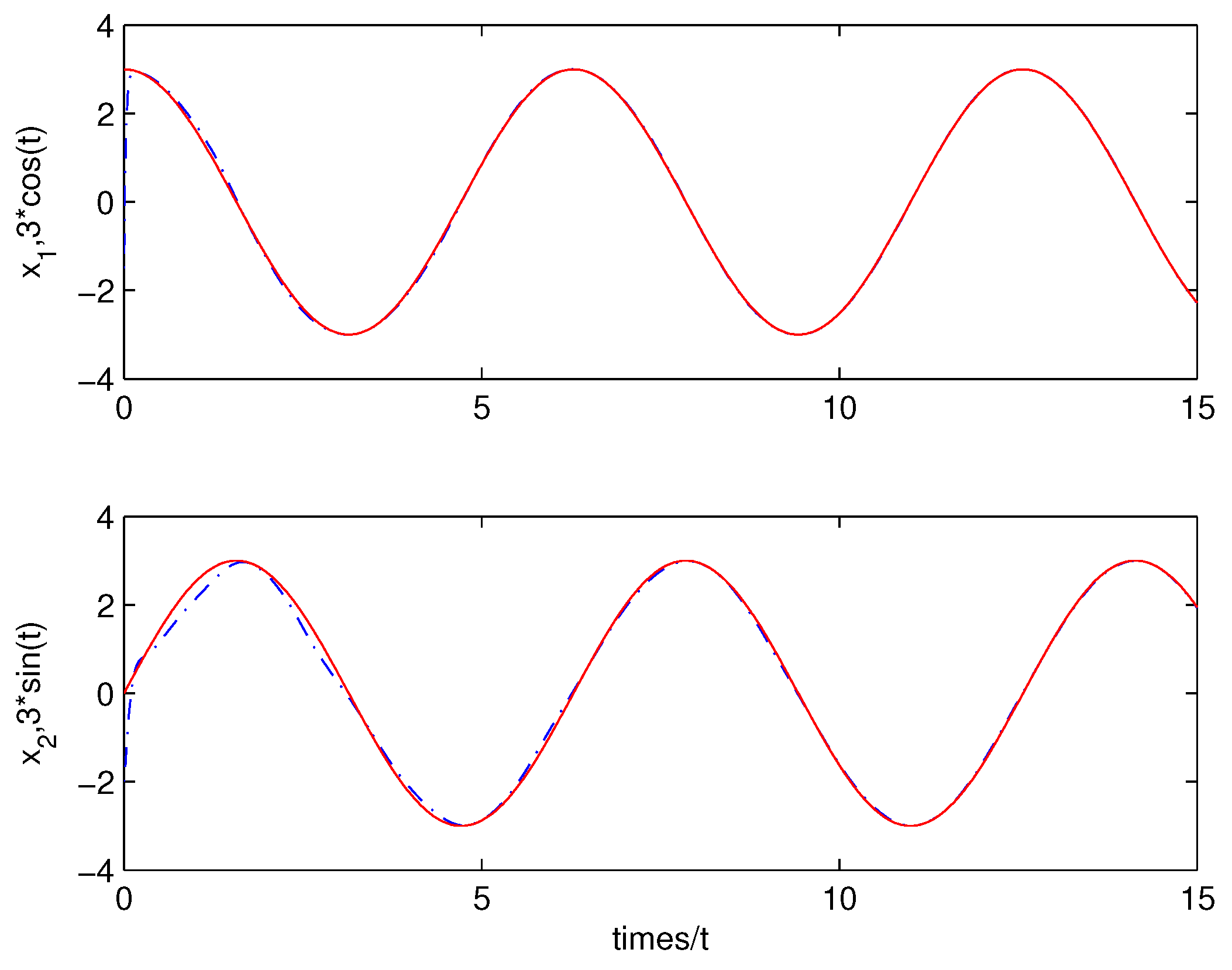
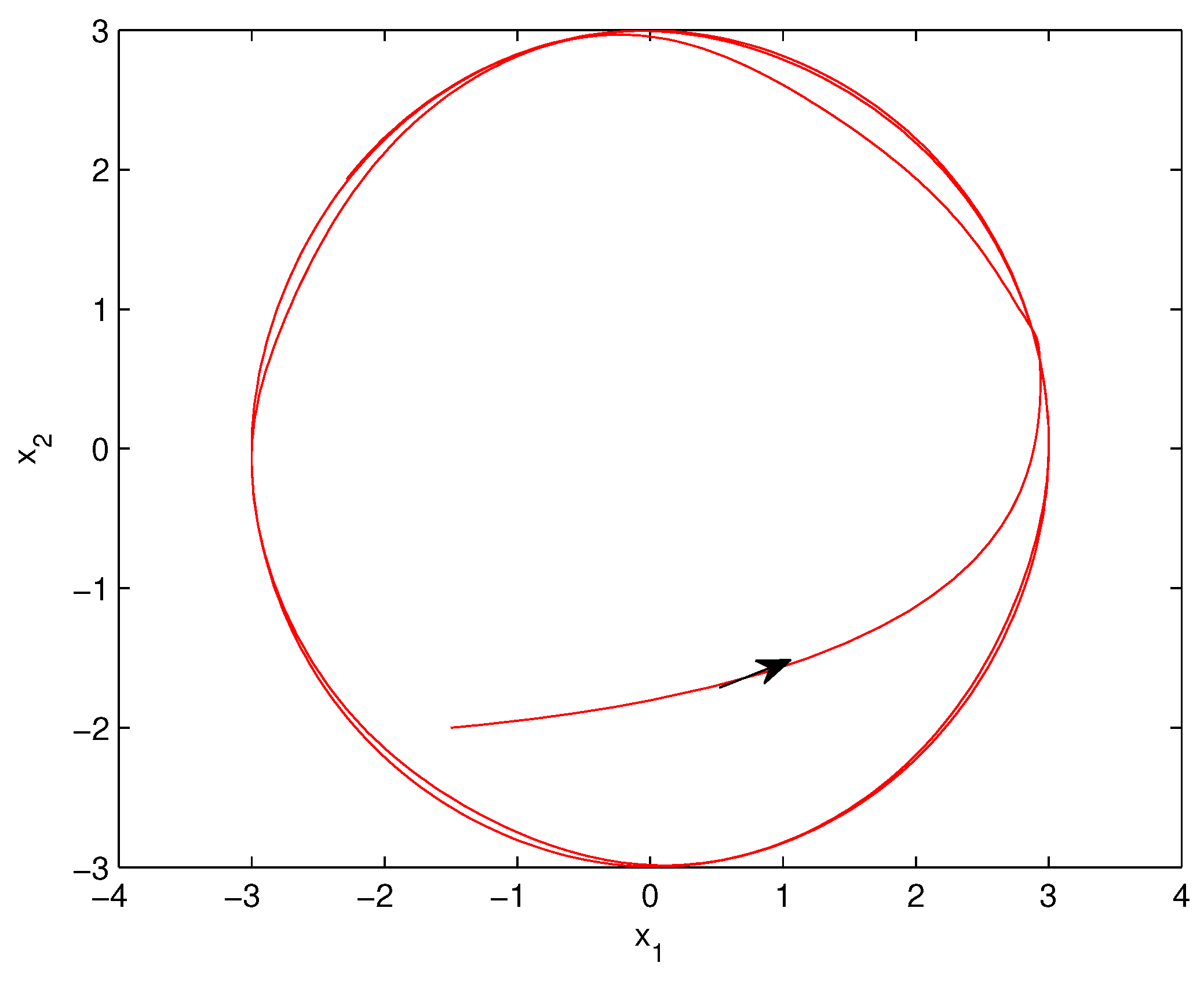
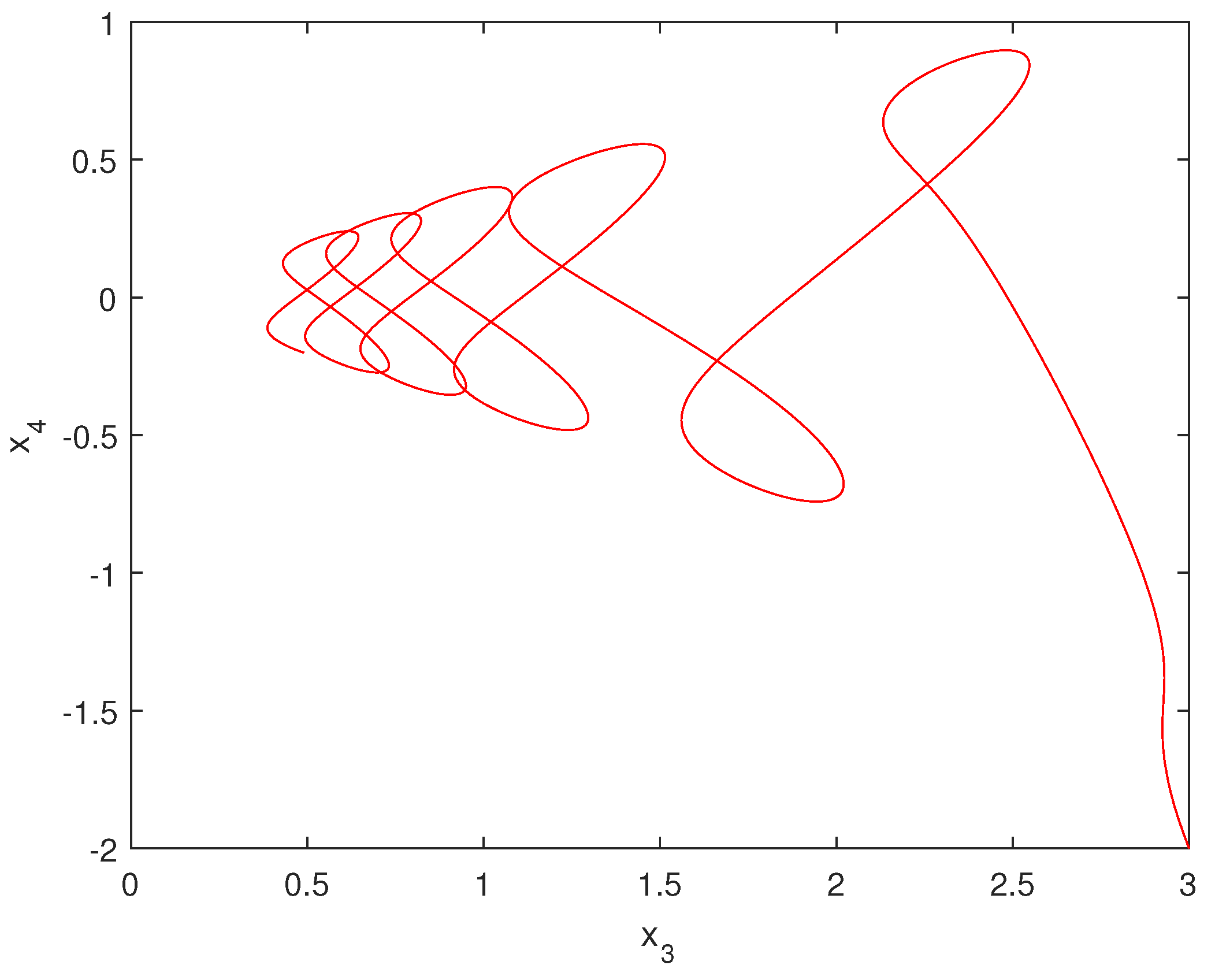
4. Numerical Examples

In the next, we take three systems for example to show how to use the proposed results in Section 3.
Example 1.
Lorenz model [22]:
w ˙ 1 = 10 ( w 2 w 1 ) w ˙ 2 = 28 w 1 w 2 w 1 w 3 w ˙ 3 = 8 3 w 3 + w 1 w 2
Let x 1 = w 1 , x 2 = w 2 , z = w 3 , then the controlled Lorenz chaotic system is expressed as follows:
x ˙ = A ( z ) x + B u ( t ) z ˙ = f ( x , z ) y = C x
where x = ( x 1 , x 2 ) T R 2 , z R 1 , u ( t ) R 1 ,
A ( z ) = 10 10 28 z 1 , B = 1 0 , C = ( 1 , 0 )
and
f ( x , z ) = 8 3 z + x 1 x 2 .
The objective is to design a controller u ( t ) which can ensure the following performance:
lim t y = c ( t ) , i . e . , lim t x 1 = 5
where c ( t ) = 5 is the given command.
The first step is to design the reference system. For the matrix A ( z ) given as (16), one feasible choice of the feedback gain K ( z ) is designed as follows:
K ( z ) = ( 0 , 10 ) .
Then, the reference system is expressed as follows:
x ˙ r = A ( z ) + B K ( z ) x r + B r c ( t )
where B r = ( 10 , 0 ) T .
The second step is to design the controller u ( t ) . According to the Equation (12), the controller is designed as
u ( t ) = K ( z ) x + B + B r c ( t ) = 10 x 2 + 10 c ( t ) .
Thus, the system (15) and the reference system (19) is synchronized, and thus y = x 1 asymptotically tracks the command c ( t ) = 5 .
In the next, with initial conditions: x ( 0 ) = ( 1 , 2 , 3 ) T , numerical simulation is made. The simulation result is shown by the following figure. From Figure 1, we can see that y ( t ) = x 1 ( t ) tends to the given command c ( t ) = 5 quickly. Figure 2 shows the state ( x 2 , x 3 ) T of the system (15) converges to a constant as t .
Example 2.
The Chen-Lee chaotic system [23]:
w ˙ 1 = w 2 w 3 + 5 w 1 w ˙ 2 = w 1 w 3 10 w 2 w ˙ 3 = 1 3 w 1 w 2 3.8 w 3
Let x 1 = w 1 , x 2 = w 2 , z = w 3 , then the controlled Chen-Lee chaotic system is expressed as follows:
x ˙ = A ( z ) x + B u ( t ) z ˙ = f ( x , z ) y = C x
where x ( t ) R 2 , z R 1 , u ( t ) R 1 ,
A ( z ) = 5 z z 10 , B = 1 0 , C = ( 1 0 ) ,
and
f ( x , z ) = 1 3 x 1 x 2 3.8 z .
The objective is to design a controller u ( t ) which can ensure the following performance:
lim t y = c ( t ) , i . e . , lim t x 1 = sin ( 3 t )
where c ( t ) = sin ( 3 t ) is the given command.
The first step is to design the reference system. For the matrix A ( z ) , one feasible choice of the feedback gain K ( z ) is obtained as follows:
K ( z ) = ( 6 , 0 ) .
Then, the reference system which is described as follows:
x ˙ r ( t ) = A ( z ) + B K ( z ( t ) ) x r + B r c ( t ) + D r c ˙ ( t )
where B r = D r = ( 1 , 0 ) T .
The second step is to design the controller u ( t ) . According to the Equation (12), the controller is designed as follows:
u ( t ) = K ( z ) x ( t ) + B + B r c ( t ) + D r c ˙ ( t ) = 6 x 1 + c ( t ) + c ˙ ( t ) .
Therefore, the system (22) and the reference system (26) is synchronized, and thus y = x 1 asymptotically tracks the command c ( t ) = sin ( 3 t ) .
In the next, with initial conditions: x ( 0 ) = ( 1 , 2 , 3 ) T , numerical simulation is made. The simulation result is shown by the following figure. From Figure 3, we can see that y = x 1 tends to the given command c ( t ) = sin ( 3 t ) quickly. Figure 4 shows the state ( x 2 , x 3 ) T of the system (22) converges to a constant as t .
Example 3.
Consider the following 4D hyper-chaotic system [24]:
w ˙ 1 = 35 ( w 2 w 1 ) + w 2 w 3 w 4 w ˙ 2 = 10 ( w 2 + w 1 ) w 1 w 3 w 4 w ˙ 3 = w 3 + w 1 w 2 w 4 w ˙ 4 = 10 w 4 + w 1 w 2 w 3
Let x 1 = w 1 , x 2 = w 2 , z 1 = w 3 , z 2 = w 4 , then the controlled system (28) is described as follows:
x ˙ = A ( z ) x ( t ) + B u ( t ) z ˙ = f ( x , z ) y = C x
where x R 2 , z R 2 , u ( t ) R 2 ,
A ( z ) = 35 35 + z 1 z 2 10 z 1 z 2 10 ,
B = C = 1 0 0 1 ,
and
f ( x , z ) = f 1 ( x , z ) f 2 ( x , z ) = z 1 + x 1 x 2 z 2 10 z 2 + x 1 x 2 z 1 .
The objective is to design a controller u ( t ) which can ensure the following performance:
lim t y ( t ) = c ( t ) , i . e . , lim t x 1 = 3 cos ( 3 t ) , lim t x 2 = 3 sin ( 3 t )
where the given command c ( t ) is given as
c ( t ) = ( c 1 ( t ) , c 2 ( t ) ) T = ( 3 cos ( t ) , 3 sin ( t ) ) T .
The first step is to design the reference system. For the matrix A ( z ) , one feasible choice of the feedback gain K ( z ) is designed as
K ( z ( t ) ) = 0 35 10 20 .
Then, the reference system which is described as
x ˙ r = A ( z ) + B K ( z ) x r ( t ) + B r c ( t ) + D r c ˙ ( t )
where D r = B and
B r = 35 0 0 10 .
The second step is to design the controller u ( t ) . According to the Equation (12), the control law is obtained as
u ( t ) = K ( z ) x + B + B r c ( t ) + D r c ˙ ( t ) = 35 x 2 10 x 1 20 x 2 + 35 c 1 ( t ) 10 c 2 ( t ) + c ˙ 1 ( t ) c ˙ 2 ( t ) .
Thus, the system (29) and the reference system (34) is synchronized, and thus y = ( x 1 , x 2 ) T asymptotically tracks the command c ( t ) = ( c 1 ( t ) , c 2 ( t ) ) T .
In the next, with initial conditions: x ( 0 ) = ( 1.5 , 2 , 3 , 2 ) T , numerical simulation is carried out. The simulation result is shown by the following two figures. From Figure 3, we can see that the states ( x 1 , x 2 ) T of the system (22) converges to the given command c ( t ) = ( 3 cos ( t ) , 3 sin ( t ) ) T quickly. From Figure 5, it can be seen that phase portrait of the states x 1 , x 2 of the system (29) converges to a circle with radius 3 quickly. Figure 6 shows phase portrait of the states ( x 1 , x 2 ) T of the system (29) converges to a circle with radius 3 as t . Figure 7 shows phase portrait of the states ( x 3 , x 4 ) T of the system (29).

5. Conclusions

The asymptotic tracking control problem of the arbitrary dimensional chaotic system has been studied in this paper. Firstly, a reference system has been presented, the output of which can asymptotically track a given command. Secondly, a both physically implementable and simple controller has been designed to ensure that the given chaotic system synchronizes the reference system, and thus the output of the given chaotic system can asymptotically track the given command. It is noted that the output of the given chaotic system can asymptotically track the arbitrary desired periodic orbit. Finally, three numerical examples have been used to show how to apply and demonstrate the validity and effectiveness of the obtained results.

Author Contributions

The first and second author of this paper deal with the numerical simulation, the third author deduces the main results, and the last author and writes this paper.

Funding

This work is supported by Shandong Natural Science Foundation [ZR2018MF016] and National Natural Science Foundation of China [61877062].

Acknowledgments

The authors would like to thank the anonymous Reviewers and the Editors for their constructive comments and suggestions, which have helped enhance the presentation of this paper.

Conflicts of Interest

The authors declare no conflict of interest. The funders had no role in the design of the study; in the collection, analyses, or interpretation of data; in the writing of the manuscript, or in the decision to publish the results.

References

  1. Ott, E.; Gerbogi, C.; Yorke, J.A. Controlling Chaos. Phys. Rev. Lett. 1990, 64, 1196–1199. [Google Scholar] [CrossRef]
  2. Pecora, L.; Carroll, T. Synchronization in Chaotic Systems. Phys. Rev. Lett. 1990, 64, 821–824. [Google Scholar] [CrossRef]
  3. Rosenblum, M.G.; Pikovsky, A.S.; Kurths, J. Phase synchronization of chaotic oscillators. Phys. Rev. Lett. 1996, 76, 1804–1807. [Google Scholar] [CrossRef] [PubMed]
  4. Rosenblum, M.G.; Pikovsky, A.S.; Kurths, J. From phase to lag synchronization in coupled chaotic oscillators. Phys. Rev. Lett. 1997, 78, 4193–4196. [Google Scholar] [CrossRef]
  5. Hu, J.; Chen, S.; Chen, L. Adaptive control for anti-synchronization of Chua’s chaotic system. Phys. Lett. A 2005, 339, 455–460. [Google Scholar] [CrossRef]
  6. Mainieri, R.; Rehacek, J. Projective synchronization in three-dimensional chaotic systems. Phys. Rev. Lett. 1999, 82, 3042–3045. [Google Scholar] [CrossRef]
  7. Ren, L.; Guo, R.W.; Vincent, U.E. Coexistence of synchronization and anti-synchronization in chaotic systems. Arch. Control Sci. 2016, 26, 69–79. [Google Scholar] [CrossRef] [Green Version]
  8. Guo, R.W. Simultaneous synchronization and anti-synchronization of two identical new 4D chaotic systems. Chin. Phys. Lett. 2011, 28, 040205. [Google Scholar] [CrossRef]
  9. Guo, R. A simple adaptive controller for chaos and hyperchaos synchronization. Phys. Lett. A 2008, 372, 5593–5597. [Google Scholar] [CrossRef]
  10. Yu, W.G. Stabilization of three-dimensional chaotic systems via single state feedback controller. Phys. Lett. A 2010, 374, 1488–1492. [Google Scholar] [CrossRef]
  11. Wang, Z.F.; Shi, X.R. Anti-synchronization of liu system and Lorenz system with known and unknown parameters. Nonlinear Dyn. 2009, 57, 425–430. [Google Scholar] [CrossRef]
  12. Al-mahbashi, G.; Md Noorani, M.S.; Bakar, S.A. Projective lag synchronization in drive-response dynamical networks with delay coupling via hybrid feedback control. Nonlinear Dyn. 2015, 82, 1569–1579. [Google Scholar] [CrossRef]
  13. Du, H.Y.; Shi, P. A new robust adaptive control method for modified function projective synchronization with unknown bounded parametric uncertainties and external disturbances. Nonlinear Dyn. 2016, 85, 355–363. [Google Scholar] [CrossRef]
  14. Liu, L.X.; Guo, R.W. Control problems of Chen-Lee system by adaptive control method. Nonlinear Dyn. 2017, 87, 503–510. [Google Scholar] [CrossRef]
  15. Guo, R.W. Projective synchronization of a class of chaotic systems by dynamic feedback control method. Nonlinear Dyn. 2017, 90, 53–64. [Google Scholar] [CrossRef]
  16. Selmic, R.R.; Lewis, F.L. Deadzone compensation in motion control systems using neural networks. IEEE Trans. Autom. Control 2000, 45, 602–613. [Google Scholar] [CrossRef] [Green Version]
  17. Selmic, R.R.; Lewis, F.L. Neural net backlash compensation with Hebbian tuning using dynamic inversion. Automatica 2001, 37, 1269–1277. [Google Scholar] [CrossRef] [Green Version]
  18. Zhou, J.; Zhang, C.; Wen, C. Robust adaptive output control of uncertain nonlinear plants with unknown backlash nonlinearity. IEEE Trans. Autom. Control 2007, 52, 503–509. [Google Scholar] [CrossRef]
  19. Yu, D.C.; Wu, A.G.; Yang, C.P. A novel sliding mode nonlinear proportional-integral control scheme for controlling chaos. Chin. Phys. 2005, 14, 914–921. [Google Scholar]
  20. Yu, D.C.; Wu, A.G.; Wang, D.Q. A simple asymptotic trajectory control of full states of a unified chaotic system. Chin. Phys. 2006, 15, 306–309. [Google Scholar]
  21. Bazhenov, V.A.; Pogorelova, O.S.; Postnikova, T.G. Intermittent transition to chaos in vibroimpact system. Appl. Math. Nonlinear Sci. 2018, 3, 475–486. [Google Scholar] [CrossRef]
  22. Lorenz, E.N. Deterministic nonperiodic flow. J. Atmos. Sci. 1963, 20, 130–141. [Google Scholar] [CrossRef]
  23. Tam, L.M.; Si Tou, W.M. Parametric study of the fractional order Chen-Lee system. Chaos Solitons Fractals 2008, 37, 817–826. [Google Scholar] [CrossRef]
  24. Qi, G.Y.; Du, S.Z.; Chen, G.R.; Chen, Z.Q.; Yuan, Z.Z. On a four-dimensional chaotic system. Chaos Solitons Fractals 2005, 23, 1671–1682. [Google Scholar] [CrossRef]
Figure 1. Shows that the state x 1 of the system (15) converges to c ( t ) = 5 as t .
Symmetry 11 00568 g001
Figure 2. Shows the state ( x 2 , x 3 ) T of the system (15) converges to a constant as t .
Symmetry 11 00568 g002
Figure 3. Shows the state x 1 of the system (22) converges to c ( t ) = sin ( 3 t ) as t .
Symmetry 11 00568 g003
Figure 4. Shows the state ( x 2 , x 3 ) T of the system (22) converges to a constant as t .
Symmetry 11 00568 g004
Figure 5. Shows the states ( x 1 , x 2 ) T of the system (22) converges to c ( t ) = ( 3 cos ( t ) , 3 sin ( t ) ) T as t .
Symmetry 11 00568 g005
Figure 6. Shows phase portrait of the states ( x 1 , x 2 ) T of the system (29) converges to a circle with radius 3 as t .
Symmetry 11 00568 g006
Figure 7. Shows phase portrait of the states ( x 3 , x 4 ) T of the system (29).
Symmetry 11 00568 g007

