A New Stability Theory for Grünwald–Letnikov Inverse Model Control in the Multivariable LTI Fractional-Order Framework

Abstract

The new general theory dedicated to the stability for LTI MIMO, in particular nonsquare, fractional-order systems described by the Grünwald–Letnikov discrete-time state–space domain is presented in this paper. Such systems under inverse model control, principally MV/perfect control, represent a real research challenge due to an infinite number of solutions to the underlying inverse problem for nonsquare matrices. Therefore, the paper presents a new algorithm for fractional-order perfect control with corresponding stability formula involving recently given H- and $\sigma$-inverse of nonsquare matrices, up to now applied solely to the integer-order plants. On such foundation a new set of stability-related tools is introduced, among them the key role played by so-called control zeros. Control zeros constitute an extension of transmission zeros for nonsquare fractional-order LTI MIMO systems under inverse model control. Based on the sets of stable control zeros a minimum-phase behavior is specified because of the stability of newly defined perfect control law described in the non-integer-order framework. The whole theory is complemented by pole-free fractional-order perfect control paradigm, a special case of fractional-order perfect control strategy. A significant number of simulation examples confirm the correctness and research potential proposed in the paper methodology.

1. Introduction

Problems concerning stability of multivariable control systems described by both transfer function and state–space frameworks have recently attracted substantial research interest. A plethora of methods providing time and frequency domain approaches meets the requirements, nevertheless there is still considerable room and growing demand for the new techniques to overcome the constantly emerging control challenges. One of the remarkable and innovative methodology seems to be strategy based on the multivariable inverse model control, according to an infinite number of solutions underlying inverse problem for nonsquare matrices. The methodology presented in this paper provides a set of stability-devoted tools, derived from inverse model control, particularly MV/perfect control. It implements and develops the idea of recently introduced the so-called control zeros, until now defined in the discrete- and continuous-time integer-order frameworks. The control zeros play here fundamental role in determining stable/unstable properties for non-integer-order systems and allow predefinition of the stable and robust MV/perfect control strategies especially for nonsquare MIMO plants with different numbers of input and output variables. It should also be noticed that control zeros have first been derived for discrete-time integer-order LTI MIMO nonsquare systems described by the input–output model in form of multivariable transfer function [1]. They were defined as the points of the complex plain which determine the stability of the closed-loop minimum variance/perfect control procedure. It has been proven that for stable control zeros the perfect control algorithm is also stable, and the system should be called a minimum-phase plant [2,3,4,5]. On the other hand, the nonminimum-phase system with unstable control zeros is associated with unstable perfect control law. Next, the control zeros were defined for continuous-time plants with a definition of the minimum-phase systems stated in relation to the parallel stable MV/perfect control law [6]. Control zeros form an extension of transmission zeros for nonsquare LTI MIMO systems being under IMC, in particular MV/perfect control/perfect regulation [7,8,9,10,11]. Like the transmission zeros defined for SISO and square MIMO systems, the control zeros are in relation to the stabilizing potential of the MV/perfect control algorithm [12,13,14]. Placement of control zeros to desirable locations guaranteeing the robustness of such law is a difficult problem that has only been solved recently [15]. Due to existence of an infinite number of solutions associated with an application of nonunique inverses involved in the control algorithm, we can freely compose the MV/perfect control signals of the closed-loop plants. The case locating the control zeros at the origin of the complex plane with no transmission zeros seems to be very interesting, and the instance is obviously called a structurally stable pole-free scenario. The paper extends the entire theory of control zeros to cover the LTI MIMO discrete-time fractional-order plants described in the G-L framework [16,17,18]. The new perfect control strategy for such a class of systems is given together with related issue of minimum/nonminimum-phase property. Since the new tool is useful for synthesis of more general non-integer systems, it can provide a strong motivation to extend it for the case of continuous time.

The paper is organized as follows. The second section presents the fractional-order system representation in the state–space domain. Next section outlines the notion of perfect control for systems defined in Section 2. The definitions of right inverses and their application in the perfect control law are indicated in Section 4. Section 5 deals with the stability of discrete-time perfect control for both integer- and fractional-order cases. The following part of the paper provides the definitions of control zeros and minimum-phase property of fractional-order plants. In this unit the fractional-order pole-free perfect control strategy is also given. Vital issues involving robustness of examined systems are discussed in the subsequent section. Simulation examples included in the eighth section confirm the significant potential offered by the proposed new method. The final section of this paper contains summary and statement of the open problems.

2. Fractional-Order State–Space System Representation

Consider an LTI fractional-order plant $S_{\mathrm{F}-\mathrm{O}}$ with $n_u$-inputs, $n_y$-outputs and n-state variable vector in discrete-time k described by

$$\left\{\begin{array}{cc}{\Delta }^{\alpha }\mathbf{x}(k+1)={\mathbf{A}}_{\mathbf{d}}\mathbf{x}\left(k\right)+\mathbf{B}\mathbf{u}\left(k\right),\hfill & \mathbf{x}\left(0\right)={\mathbf{x}}_{\mathbf{0}}\hfill \\ \mathbf{y}\left(k\right)=\mathbf{C}\mathbf{x}\left(k\right)\hfill \end{array}\right.,$$

(1)

where the discrete-time difference operator ${\Delta }^{\alpha }$ is the G-L difference of an arbitrary fractional-order $\alpha$, with $0<\alpha <2$, as follows

$${\Delta }^{\alpha }\mathbf{x}\left(k\right)=\sum _{j=0}^k{(-1)}^j\left(\begin{array}{c}\alpha \\ j\end{array}\right)\mathbf{x}(k-j),$$

(2)

where

$$\left(\begin{array}{c}\alpha \\ j\end{array}\right)=\left\{\begin{array}{cc}1\hfill & j=0\hfill \\ \frac{\alpha (\alpha -1)\dots (\alpha -j+1)}{j!}\hfill & j>0\hfill \end{array}\right..$$

(3)

Assume also the system is controllable and observable. Please note that for $\alpha =1$ the plant as in Equations (1)–(3) comes down to the classical integer-order one $S_{\mathrm{I}-\mathrm{O}}$ in the following form

$$\left\{\begin{array}{cc}\mathbf{x}(k+1)=\mathbf{A}\mathbf{x}\left(k\right)+\mathbf{B}\mathbf{u}\left(k\right),\hfill & \mathbf{x}\left(0\right)={\mathbf{x}}_{\mathbf{0}}\hfill \\ \mathbf{y}\left(k\right)=\mathbf{C}\mathbf{x}\left(k\right).\hfill \end{array}\right..$$

(4)

In both non-integer- and integer-order cases, we must assume that $\mathbf{A}\in {\mathbb{R}}^{n\times n}$, $\mathbf{B}\in {\mathbb{R}}^{n\times n_u}$, $\mathbf{C}\in {\mathbb{R}}^{n_y\times n}$ with ${\mathbf{A}}_{\mathbf{d}}=\mathbf{A}-{\mathbf{I}}_{\mathbf{n}}$, whereas ${\mathbf{I}}_{\mathbf{n}}$ is the identity n-matrix.

3. Fractional-Order Perfect Control

Observe that the Equation (2) can be rewritten into the form

$$\mathbf{x}(k+1)={\Delta }^{\alpha }\mathbf{x}(k+1)-\sum _{j=1}^{k+1}{(-1)}^j\left(\begin{array}{c}\alpha \\ j\end{array}\right)\mathbf{x}(k-j+1).$$

(5)

Consequently, after minimizing the (noise-free) control performance index for the plants with time delay $d=1$

$$J\left(u\right)=\sum _{k=0}^{\infty }\left\{{\left[\mathbf{y}(k+1)-{\mathbf{y}}_{\mathbf{ref}}(k+1)\right]}^{\mathrm{T}}\left[\mathbf{y}(k+1)-{\mathbf{y}}_{\mathbf{ref}}(k+1)\right]\right\},$$

(6)

where

$$\mathbf{y}(k+1)=\mathbf{C}\left[{\Delta }^{\alpha }\mathbf{x}(k+1)-\sum _{j=1}^{k+1}{\left(-1\right)}^j\left(\begin{array}{c}\alpha \\ j\end{array}\right)\mathbf{x}(k-j+1)\right],$$

(7)

and ${\mathbf{y}}_{\mathbf{ref}}(k+1)$ are the one-step deterministic output predictor and reference/setpoint, respectively, we obtain the perfect control law [19]

$$\begin{array}{c}\mathbf{u}\left(k\right)={\left(\mathbf{CB}\right)}^{\mathrm{R}}[{\mathbf{y}}_{\mathbf{ref}}(k+1)-\mathbf{C}{\mathbf{A}}_{\mathbf{d}}\mathbf{x}\left(k\right)\hfill \end{array}\left.+\mathbf{C}\sum _{j=1}^{k+1}{(-1)}^j\left(\begin{array}{c}\alpha \\ j\end{array}\right)\mathbf{x}(k-j+1)\right],$$

(8)

where symbol ’$\mathrm{R}$’ denotes any right inverse of product of $\mathbf{CB}$ [8].

Remark 1.

The Formula (8) is only valid for systems with regard to several input and output variables. We must take into account the so-called right-invertible plants fulfilling the condition $n_u\ge n_y$. This problem is explained in detail further on in the paper.

Remark 2.

It is worth noticing that the non-integer-order prefect control law (8) can also be applied to systems blurred by zero-mean uncorrelated disturbance in form of white noise. However, minimum variance control problem goes beyond the scope of this paper.

Remark 3.

For $\alpha =1$ the Equation (8) reduces to the perfect control of integer-order systems as follows

$$\mathbf{u}\left(k\right)={\left(\mathbf{CB}\right)}^{\mathrm{R}}[{\mathbf{y}}_{\mathbf{ref}}(k+1)-\mathbf{C}\mathbf{A}\mathbf{x}\left(k\right)].$$

(9)

With the notion of issues of both fractional-order system representation and relevant perfect control law, we can proceed to the problem of application of the appropriate inverse of the product $\mathbf{CB}$.

4. An Application of Parameter Matrix Right Inverses into Fractional-Order Perfect Control Law

4.1. Selection of Nonunique Right Inverse

The issues regarding the stability and robustness of MV/perfect control for LTI MIMO integer-order discrete-time systems in state–space domain are subject to increasingly intensive scientific exploration [20,21]. The search for various methods is being conducted in particular to obtain new classes of right inverses. Until now, the mostly used and widely presented in the literature is minimum-norm right T-inverse [22,23]. T-inverse considered, however, as the ‘minimum-energy’ inverse, cannot be applied regarding a wide class of cases where the control inputs remain unstable under perfect control law. The recently introduced $\sigma$-inverse and H-inverse with various types of so-called degrees of freedom offer powerful tools to be applied regarding the above class of problems [24,25]. It is interesting that the first inverse constitutes an extension of minimum-norm right T-inverse in which degrees of freedom are organized as separate matrices being both in parameter as well as polynomial form. On the other hand, the second of the inverses is based on well-known SVD factorization. That approach gives the opportunity to impact on the perfect control strategy by influencing matrices obtained from SVD factorization in form of parameter or polynomial degrees of freedom as well. The tools mentioned above, previously employed to integer-order systems, are transferred to fractional-order perfect control of LTI MIMO discrete-time state–space systems [26]. It is remarkable that the concept of engaging the inverses of parameter matrices to increasing the robustness of multivariable discrete-time fractional-order perfect control structures in a state–space forms a new and original idea developed by these authors, not presented so far. Therefore, it is an attempt to synthesis of discrete-time fractional-order perfect control with regard of its stability and robustness. To obtain that objective, the recently devised a fractional-order multivariable discrete-time perfect control algorithm, in particular dedicated to the so-called nonsquare state–space systems, i.e., systems with different number of input and output variables, is used [19]. The simulations performed into perfect control involve parameter $\sigma$-inverse and H-inverse. The results of research conducted in MATLAB/Simulink environment show that use of appropriate inverse machinery may determine stability and, consequently, minimum-phase property of the non-integer plants. The definitions of the right inverses presented in the next section constitute the essential element for calculation of the control zeros, as they affect the properties of the fractional-order perfect control systems discussed in this paper.

4.2. Inverses of Nonsquare (Parameter) Matrices

Let us start our considerations with the definitions of the classical minimum-norm inverses of polynomial matrix $\underline{\mathbf{W}}\left(q^{-1}\right)$ in the backward shift operator $q^{-1}$, afterwards called T-inverse [8,27,28,29,30,31]. The following two definitions are dedicated to full and non-full normal rank polynomial matrices $\underline{\mathbf{W}}\left(q^{-1}\right)$, respectively.

Definition 1.

Let the polynomial matrix $\underline{\mathbf{W}}\left(q^{-1}\right)=\underline{\mathbf{w}}{}_{\mathbf{0}}+\underline{\mathbf{w}}{}_{\mathbf{1}}$$q^{-1}+\dots +\underline{\mathbf{w}}{}_{\mathbf{m}}$$q^{-m}$ be of full normal rank $n_y$ (or $n_u$). The (unique) minimum-norm right (or the least-squares left) T-inverse of $\underline{\mathbf{W}}\left(q^{-1}\right)$ is defined as ${\underline{\mathbf{W}}}_0^{\mathrm{R}}\left(q^{-1}\right)={\underline{\mathbf{W}}}^{\mathrm{T}}\left(q^{-1}\right){\left[\underline{\mathbf{W}}\left(q^{-1}\right){\underline{\mathbf{W}}}^{\mathrm{T}}\left(q^{-1}\right)\right]}^{-1}$ (or ${\underline{\mathbf{W}}}_0^{\mathrm{L}}\left(q^{-1}\right)={\left[{\underline{\mathbf{W}}}^{\mathrm{T}}\left(q^{-1}\right)\underline{\mathbf{W}}\left(q^{-1}\right)\right]}^{-1}{\underline{\mathbf{W}}}^{\mathrm{T}}\left(q^{-1}\right)$).

Definition 2.

Let the polynomial matrix $\underline{\mathbf{W}}\left(q^{-1}\right)=\underline{\mathbf{w}}{}_{\mathbf{0}}+\underline{\mathbf{w}}{}_{\mathbf{1}}{\mathbf{q}}^{-\mathbf{1}}+\dots +\underline{\mathbf{w}}{}_{\mathbf{m}}{\mathbf{q}}^{-\mathbf{m}}$ of non-full normal rank r be skeleton-factorized as $\underline{\mathbf{W}}\left(q^{-1}\right)=\underline{\mathbf{C}}\left(q^{-1}\right)\underline{\mathbf{D}}\left(q^{-1}\right)$, where $dim\left[\underline{\mathbf{W}}\left(q^{-1}\right)\right]=n_y\times n_u$, $dim\left[\underline{\mathbf{C}}\left(q^{-1}\right)\right]=n_y\times r$, $dim\left[\underline{\mathbf{D}}\left(q^{-1}\right)\right]=r\times n_u$. The (unique) Moore-Penrose T-inverse of $\underline{\mathbf{W}}\left(q^{-1}\right)$ is defined as ${\underline{\mathbf{W}}}_0^{\#}\left(q^{-1}\right)={\underline{\mathbf{D}}}_0^{\mathrm{R}}\left(q^{-1}\right){\underline{\mathbf{C}}}_0^{\mathrm{L}}\left(q^{-1}\right)$, where ${\underline{\mathbf{D}}}_0^{\mathrm{R}}\left(q^{-1}\right)={\underline{\mathbf{D}}}^{\mathrm{T}}\left(q^{-1}\right){\left[\underline{\mathbf{D}}\left(q^{-1}\right){\underline{\mathbf{D}}}^{\mathrm{T}}\left(q^{-1}\right)\right]}^{-1}$ and ${\underline{\mathbf{C}}}_0^{\mathrm{L}}\left(q^{-1}\right)={\left[{\underline{\mathbf{C}}}^{\mathrm{T}}\left(q^{-1}\right)\underline{\mathbf{C}}\left(q^{-1}\right)\right]}^{-1}{\underline{\mathbf{C}}}^{\mathrm{T}}\left(q^{-1}\right)$.

Remark 4.

The systems taken into account are parameter plants which constitute a special case of polynomial ones.

An extension of the unique right T-inverse is nonunique right $\sigma$-inverse including degrees of freedom. The newest definition of $\sigma$-inverse can be found in Ref. [32] in the form of the following corollary

Corollary 1.

Let the polynomial matrix $\underline{\mathbf{W}}\left(q^{-1}\right)=\underline{\mathbf{w}}{}_{\mathbf{0}}+\underline{\mathbf{w}}{}_{\mathbf{1}}$$q^{-1}+\dots +\underline{\mathbf{w}}{}_{\mathbf{m}}$$q^{-m}$ be of full normal rank $n_y$ (or $n_u$) and let $z^{\mathrm{s}}\underline{\beta }\left(z^{-1}\right)=\underline{\beta }\left(z\right)\in {\mathbb{R}}^{n_y\times n_u}\left[z\right]$ be arbitrary, including an arbitrary order s. Assume additionally that the product $\underline{\mathbf{W}}\left(q^{-1}\right){\underline{\beta }}^{\mathrm{T}}\left(q^{-1}\right)$ is of full normal rank $n_y$ (or $n_u$). Then a right σ-inverse can be defined as

$${\underline{\mathbf{W}}}^{\mathrm{R}}\left(q^{-1}\right)={\underline{\beta }}^{\mathrm{T}}\left(q^{-1}\right){\left[\underline{\mathbf{W}}\left(q^{-1}\right){\underline{\beta }}^{\mathrm{T}}\left(q^{-1}\right)\right]}^{-1}.$$

(10)

Remark 5.

Naturally, the presented polynomial matrix right σ-inverse reduces to the parameter one for $\underline{\mathbf{W}}\left(q^{-1}\right)=\underline{\mathbf{w}}{}_{\mathbf{0}}$ and takes the form

$${\underline{\mathbf{W}}}^{\mathrm{R}}\left(q^{-1}\right)={\beta }^{\mathrm{T}}{\left[\underline{\mathbf{W}}\left(q^{-1}\right){\beta }^{\mathrm{T}}\right]}^{-1},$$

(11)

with parameter degrees of freedom β. Some issues concerning β with parameter matrices can be found in [33].

Remark 6.

It is clear now that in Equation (11) the ${\mathbf{W}}^{\mathrm{R}}$ should be used instead of ${\underline{\mathbf{W}}}^{\mathrm{R}}\left(q^{-1}\right)$, as well as $\mathbf{W}$ instead of $\underline{\mathbf{W}}\left(q^{-1}\right)$.

Remark 7.

For $\underline{\beta }\left(q^{-1}\right)=\underline{\mathbf{W}}\left(q^{-1}\right)$ the σ-inverse specializes to the T-inverse and in the parameter case is as follows

$${\left(\mathbf{W}\right)}_0^{\mathrm{R}}={\mathbf{W}}^{\mathrm{T}}{\left[\mathbf{W}{\mathbf{W}}^{\mathrm{T}}\right]}^{-1},$$

(12)

where symbol ${(.)}_0^{\mathrm{R}}$ denotes the unique minimum-norm right T-inverse.

Finally, the recently introduced nonunique parameter right H-inverse based on SVD factorization is shown below.

Theorem 1

([24]). Consider an $m\times n$ matrix $\mathbf{A}$ being of full rank m under the SVD decomposition ${\mathbf{A}=\mathbf{U}\mathsf{\Sigma }\mathbf{V}}^{\mathrm{T}}$, where $\mathbf{U}$ and $\mathbf{V}$ are unitary matrices and $\mathsf{\Sigma }=\left[\begin{array}{cc}diag({\sigma }_1,\dots ,{\sigma }_{\mathrm{m}}& {\mathbf{0}}_{m\times (n-m)})\end{array}\right]$ includes eigenvalues of $\mathbf{A}$. Then the right matrix H-inverse of $\mathbf{A}$ can be given as

$${\mathbf{A}}^{\mathrm{R}}={\left({\mathbf{V}}^{\mathrm{T}}\right)}^{-\mathbf{1}}{\mathsf{\Sigma }}^{\mathrm{R}}{\mathbf{U}}^{-\mathbf{1}},$$

(13)

where ${\mathsf{\Sigma }}^{\mathrm{R}}=\left[\begin{array}{c}{\mathsf{\Sigma }}_{\mathbf{m}}^{-1}\\ \mathbf{L}\end{array}\right]$ and ${\mathsf{\Sigma }}_{\mathbf{m}}^{-1}=diag(\frac{1}{{\sigma }_1},\dots ,\frac{1}{{\sigma }_{\mathrm{m}}})$ while $\mathbf{L}\in {\mathbb{R}}^{(n-m)\times m}\left(q^{-1}\right)$ is an arbitrary matrix polynomial in the backward shift operator domain.

Remark 8.

As in preceding case, the presented polynomial matrix $\mathbf{L}\left(q^{-1}\right)$, including degrees of freedom, can be reduced to the parameter form $\mathbf{L}$.

Remark 9.

For $\mathbf{L}=\mathbf{0}$ we obtain the classical minimum-norm right or least-square left T-inverse [34].

With the needed notion of polynomial inverses and their parameter representations, we are able to proceed with the implementation of right T-, $\sigma$- and H-inverse into the fractional-order perfect control law as in Equation (8), which is the subject of the subsequent section.

4.3. Employment of Right Inverses into Fractional-Order Perfect Control Law

Starting to consider the implementation outlined in former section right inverses into Equation (8) we must assume that the product of $\mathbf{CB}$ is of full rank. First, we take into account the classical minimum-norm T-inverse. It is important to note that the minimum-norm T-inverse represents a special case of a more general one related to $\sigma$-inverse (see Remark 7). Therefore, regarding Equation (8), the fractional-order perfect control formula for LTI MIMO discrete-time systems in state–space can be presented in the following form

$$\begin{array}{c}\mathbf{u}\left(k\right)={{\left(\mathbf{CB}\right)}^{\mathrm{T}}\left[\mathbf{CB}{\left(\mathbf{CB}\right)}^{\mathrm{T}}\right]}^{-1}\left[{\mathbf{y}}_{\mathbf{ref}}(k+1)-{\mathbf{CA}}_{\mathbf{d}}\mathbf{x}\left(k\right)\right.\hfill \end{array}\left.+\mathbf{C}\sum _{j=1}^{k+1}{\left(-1\right)}^j\left(\begin{array}{c}\alpha \\ j\end{array}\right)\mathbf{x}(k-j+1)\right].$$

(14)

Secondly, to implement $\sigma$-inverse, we rewrite Equation (8) according to the Corollary 1 with corresponding remarks as follows

$$\begin{array}{c}\mathbf{u}\left(k\right)={{\beta }^{\mathrm{T}}\left[\mathbf{CB}{\beta }^{\mathrm{T}}\right]}^{-1}\left[{\mathbf{y}}_{\mathbf{ref}}(k+1)-{\mathbf{CA}}_{\mathbf{d}}\mathbf{x}\left(k\right)\right.\hfill \end{array}\left.+\mathbf{C}\sum _{j=1}^{k+1}{\left(-1\right)}^j\left(\begin{array}{c}\alpha \\ j\end{array}\right)\mathbf{x}(k-j+1)\right],$$

(15)

with parameter degrees of freedom matrix $\beta$ of $n_y\times n_u$ dimension.

Eventually, the SVD-based H-inverse formula defined in the Theorem 1 is applied to Equation (8). Hence, we obtain fractional-order perfect control law related to H-inverse in the following form

$$\begin{array}{c}\mathbf{u}\left(k\right)={\left({\mathbf{V}}_{\mathbf{CB}}^{\mathrm{T}}\right)}^{-1}{\mathsf{\Sigma }}_{\mathbf{CB}}^{\mathrm{R}}{\mathbf{U}}_{\mathbf{CB}}^{-1}\left[{\mathbf{y}}_{\mathbf{ref}}(k+1)-{\mathbf{CA}}_{\mathbf{d}}\mathbf{x}\left(k\right)\right.\hfill \end{array}\left.+\mathbf{C}\sum _{j=1}^{k+1}{\left(-1\right)}^j\left(\begin{array}{c}\alpha \\ j\end{array}\right)\mathbf{x}(k-j+1)\right].$$

(16)

With the notion of the three different forms of fractional-order perfect control law we need to compile necessary conditions, as presented in the next section.

4.4. Necessary Conditions for Application of Right Inverses to the Product of $\mathbf{CB}$

Taking into account the nonsquare MIMO systems with different number of input and output variables, the problem of the inverse of nonsquare matrices arises since the perfect control bases on the IMC structure. The selection of (non)unique right inverses for nonsquare MIMO systems is essential for the problem of the stability of perfect control discussed in the next sections. Because of the fact that we consider plants with $n_u\ne n_y$, the product of $\mathbf{CB}$ must be of full rank. For non-full rank $\mathbf{CB}$ product the prefect control does not exist [8]. Therefore, first it must be assumed that the product of $\mathbf{CB}$ is only of full rank $n_y$. In fact, the right-invertible systems in which input variables outnumber the output ones ($n_u>n_y$) should be taken into account. For left-invertible systems, i.e., plants with $n_u<n_y$, the perfect control cannot be established. These two requirements constitute the basic conditions for the adequate application of (non)unique inverses.

Moreover, the issues regarding the regular inverse of the square systems, i.e. systems with $n_u=n_y$, are not touched in this paper as the unique T-inverse and nonunique $\sigma$ and H inverses reduce to the regular one. For square systems, including the SISO ones, the regular unique matrix inverse of $\mathbf{CB}$ must be applied. Such an inverse does not have degrees of freedom, which are crucial for the subject of the paper.

We can also note that the minimum-norm T-inverse applied in (non-)integer-order perfect control problems in many cases may cause an instability of the whole control system. Therefore, in perfect control robustness research there is a need to employ other nonunique inverses, for example said $\sigma$-inverse or H-inverse implemented in Formulas (15) and (16), respectively. Actually, the application of the other right inverses could be related to the problem of control zeros placement and finally determined by the appropriate selection of the degrees of freedom originated from the above-mentioned inverses. The problem of the instability of multivariable fractional-order perfect control systems defined in discrete-time state–space framework is discussed in the following sections and illustrated by simulation examples.

5. Stability of Fractional-Order Discrete-Time Perfect Control

The problem of stability of multivariable integer-order perfect control systems, described by both transfer function and state–space frameworks, is related to the so-called control zeros [1,6]. Therefore, it is important to consider the control zeros as the vital element connected with the perfect control stability. Thus, the location of different sets of control zeros, being an extension of transmission zeros for the nonsquare systems, in the complex plane can be selected based on the application of various nonunique right inverses. It is crucial that in this study we use a similar paradigm as in the case of integer-order plants to determine the stability of perfect control for LTI MIMO fractional-order systems in state–space framework. As the right inverses are essential during the design of robust perfect control strategy, they can be treated as an effective tool for robustification of MV/perfect control strategies.

5.1. Integer-Order Instance

The stability of classical integer-order discrete-time deterministic perfect control law for state–space right-invertible systems described as follows

$$\left\{\begin{array}{c}\mathbf{x}(k+1)=\mathbf{A}\mathbf{x}\left(k\right)+\mathbf{Bu}\left(k\right)\hfill \\ \mathbf{y}\left(k\right)=\mathbf{C}\mathbf{x}\left(k\right)\hfill \end{array}\right.\mathbf{x}\left(0\right)={\mathbf{x}}_{\mathbf{0}},$$

(17)

where

$$\mathbf{u}\left(k\right)=-{\mathbf{K}}_{\mathbf{I}-\mathbf{O}}\mathbf{x}\left(k\right),$$

(18)

while

$${\mathbf{K}}_{\mathbf{I}-\mathbf{O}}={\left(\mathbf{CB}\right)}^{\mathrm{R}}\mathbf{CA},$$

(19)

(see Equation (9) for ${\mathbf{y}}_{\mathbf{ref}}=\mathbf{0}$) is determined by the well-known formula [27]

$$det(z{\mathbf{I}}_{\mathbf{n}}-\mathbf{A}+{\mathbf{BK}}_{\mathbf{I}-\mathbf{O}}).$$

(20)

Remark 10.

For the simplicity of the conducted research study we take into account the consideration that ${\mathbf{y}}_{\mathbf{ref}}=\mathbf{0}$, as it does not distort the perfect control stability theorem in the general case. This statement is confirmed by the following theorem.

Theorem 2.

Let us consider systems described by Equation (17). The Formula (20) can be applied to the perfect control laws as in Equation (9) and (18).

Proof. 

Immediately, after substitution Equation (9) into the state equation of Formula (17) we obtain

$$\mathbf{x}(k+1)=(\mathbf{A}-{\mathbf{BK}}_{\mathbf{I}-\mathbf{O}})\mathbf{x}\left(k\right)+\mathbf{B}{\left(\mathbf{CB}\right)}^{\mathrm{R}}{\mathbf{y}}_{\mathbf{ref}}(k+1),$$

(21)

where the second part of the right side of equation does not influence the stability. □

Remark 11.

Observe that the same results can be achieved for plants with a time delay $d>1$.

Following the introduction of issues related to integer-order systems, the more general fractional-order case is presented in the next section.

5.2. Fractional-Order Instance

Consider the discrete-time fractional-order plants defined by Equations (1)–(3). As mentioned above, the stability of such systems, as the superclass of integer-order case, should be analyzed in a corresponding manner to integer-order ones. Thus, by analogy, we assume that the whole machinery of Section 5.1 can be successfully transferred to the non-integer-order instance. Therefore, Equation (8) should be taken into account to identify the matrix ${\mathbf{K}}_{\mathbf{F}-\mathbf{O}}$. Consequently, after a few manipulations, the Equation (8) with ${\mathbf{y}}_{\mathbf{ref}}=\mathbf{0}$ can be transformed into the following formula

$$\begin{array}{c}\mathbf{u}\left(k\right)=\hfill \end{array}-{\left(\mathbf{CB}\right)}^{\mathrm{R}}\mathbf{C}\left[{\mathbf{A}}_{\mathbf{d}}-{\mathbf{I}}_{\mathbf{n}}\sum _{j=1}^{k+1}{(-1)}^j\left(\begin{array}{c}\alpha \\ j\end{array}\right)q^{-j+1}\right]\mathbf{x}\left(k\right),$$

(22)

where q is the backward shift operator. Finally, the matrix ${\mathbf{K}}_{\mathbf{F}-\mathbf{O}}$ of fractional-order closed-loop perfect control systems is represented as follows

$${\mathbf{K}}_{\mathbf{F}-\mathbf{O}}={\left(\mathbf{C}\mathbf{B}\right)}^{\mathrm{R}}\mathbf{C}\left[{\mathbf{A}}_{\mathbf{d}}-{\mathbf{I}}_{\mathbf{n}}\sum _{j=1}^{k+1}{(-1)}^j\left(\begin{array}{c}\alpha \\ j\end{array}\right)q^{-j+1}\right].$$

(23)

With the required tools, let us try to introduce the theorem related to the stability of non-integer-order plants.

Theorem 3.

Let the LTI MIMO discrete-time fractional-order systems $S_{\mathrm{F}-\mathrm{O}}$ as in Equations (1)–(3) is described by G-L framework. Then a stability region of the perfect control defined by Equation (8) is restricted by the following formula

$$\begin{array}{c}det\left(z{\mathbf{I}}_{\mathbf{n}}-\left[{\mathbf{I}}_{\mathbf{n}}-\mathbf{B}{\left(\mathbf{CB}\right)}^{\mathrm{R}}\mathbf{C}\right]\right.\hfill \end{array}\left.\left[{\mathbf{A}}_{\mathbf{d}}-{\mathbf{I}}_{\mathbf{n}}\sum _{j=1}^{k+1}{\left(-1\right)}^j\left(\begin{array}{c}\alpha \\ j\end{array}\right)z^{-j+1}\right]\right),$$

(24)

where z is the Laplace operator.

Proof. 

After substitution of the prefect control law (22) to the plants $S_{\mathrm{F}-\mathrm{O}}$ defined by Equation (1) and altered by Formula (5) we obtain

$$\begin{array}{cc}\hfill & \begin{array}{c}\mathbf{x}(k+1)+\sum _{j=1}^{k+1}{(-1)}^j\left(\begin{array}{c}\alpha \\ j\end{array}\right)\mathbf{x}(k-j+1)={\mathbf{A}}_{\mathbf{d}}\mathbf{x}\left(k\right)\hfill \end{array}\hfill \\ \hfill & +\mathbf{B}{\left(\mathbf{CB}\right)}^{\mathrm{R}}\mathbf{C}\left[{\mathbf{A}}_{\mathbf{d}}+{\mathbf{I}}_{\mathbf{n}}\sum _{j=1}^{k+1}{(-1)}^j\left(\begin{array}{c}\alpha \\ j\end{array}\right)q^{-j+1}\right]\mathbf{x}\left(k\right),\hfill \end{array}$$

(25)

and, finally, a simplifed form is derived, as follows

$$\begin{array}{c}\mathbf{x}(k+1)=\left({\mathbf{I}}_{\mathbf{n}}-\mathbf{B}{\left(\mathbf{CB}\right)}^{\mathrm{R}}\mathbf{C}\right)\hfill \end{array}\left(\left[{\mathbf{A}}_{\mathbf{d}}-{\mathbf{I}}_{\mathbf{n}}\sum _{j=1}^{k+1}{(-1)}^j\left(\begin{array}{c}\alpha \\ j\end{array}\right)q^{-j+1}\right]\right)\mathbf{x}\left(k\right).$$

(26)

Thus, transferring Equation (26) to the z-domain we receive the subsequent statement

$$\begin{array}{c}\mathbf{X}\left(z\right)z=\left({\mathbf{I}}_{\mathbf{n}}-\mathbf{B}{\left(\mathbf{CB}\right)}^{\mathrm{R}}\mathbf{C}\right)\hfill \end{array}\left(\left[{\mathbf{A}}_{\mathbf{d}}-{\mathbf{I}}_{\mathbf{n}}\sum _{j=1}^{k+1}{(-1)}^j\left(\begin{array}{c}\alpha \\ j\end{array}\right)z^{-j+1}\right]\right)\mathbf{X}\left(z\right),$$

(27)

which holds the Equation (24). □

Remark 12.

Observe that Equation (24) corresponds to the succeeding expression

$$det(z{\mathbf{I}}_{\mathbf{n}}-{\mathbf{A}}_{\mathbf{F}-\mathbf{O}}+{\mathbf{BK}}_{\mathbf{F}-\mathbf{O}}),$$

(28)

where ${\mathbf{K}}_{\mathbf{F}-\mathbf{O}}$ is defined by the statement (23) and

$${\mathbf{A}}_{\mathbf{F}-\mathbf{O}}=\left({\mathbf{A}}_{\mathbf{d}}-{\mathbf{I}}_{\mathbf{n}}\sum _{j=1}^{k+1}{(-1)}^j\left(\begin{array}{c}\alpha \\ j\end{array}\right)\mathbf{x}(j-k+1)\right).$$

(29)

Of course, Equation (28) for $\alpha =1$ reduces to the Formula (20) dedicated to the integer-order perfect control law.

Remark 13.

Naturally, the number of roots of Equation (24) or Formula (28) must be understood in terms of simulation horizon k selected by the designer.

Concluding, let us formulate the practical theorem which allows us in a simple way to transfer formulas between integer- and non-integer-order domains.

Theorem 4.

The equations defined by integer- and non-integer-order frameworks can be considered in a similar manner under formula

$$\mathbf{A}={\mathbf{A}}_{\mathbf{F}-\mathbf{O}}.$$

(30)

Proof. 

Immediately, after using Equation (30). □

Remark 14.

The results, which were obtained, are still valid for stochastic case of perfect control, i.e., the minimum variance control (MVC).

Once we know the major issues involving the stability area of fractional-order perfect control system we can proceed to define the control zeros being the main goal of this paper.

6. Control Zeros and Minimum-Phase Property

The idea of control zeros was first introduced for discrete-time LTI MIMO integer-order plants described by the input–output model [1] and extended to cover the continuous-time systems [6]. Control zeros were defined as the points of the respective complex plane which indicated the stable/unstable property of the MV/perfect control strategy. For square systems, the set of control zeros was calculated by the application of the regular inverse to some matrix involving the dynamic description of the analyzed plant. In the cases of nonsquare plants with different number of input–output variables the above-mentioned control zeros were determined by employing unique/nonunique inverses, e.g., given in Section 4.2. Therefore, a proper set of inverses should be selected to make the IMC structure stable/unstable.

The proposition to apply the same paradigm to perfect control fractional-order plants is presented in the following sections.

6.1. Control Zeros

Definition 3.

Consider a discrete-time LTI MIMO fractional-order system $S_{\mathrm{F}-\mathrm{O}}$ described by G–L state–space framework with product of $\mathbf{CB}$ being right-invertible. The complex number $\zeta \in \mathbb{C}$ is called a control zero of the plant $S_{\mathrm{F}-\mathrm{O}}$ iff it is a root of Formulas (24) or (28).

Observe that similarly to the case of the LTI MIMO integer-order plants defined by the input–output models, the control zeros determine the stability of MV/perfect control formula. If the control zeros are located outside the unit circle the above-mentioned algorithm is unstable and, contrary, if they are placed inside the unit disk, the said control remains asymptotically stable. The statement fulfills the classical stability paradigm of discrete-time systems. Moreover, according to the Remark 13, several control zeros must be respected regarding time horizon k. This feature is presented by the following theorem and confirmed by simulation examples of Section 8.

Theorem 5.

Consider an LTI fractional-order plant ${\mathrm{S}}_{\mathrm{F}-\mathrm{O}}$ with $n_u$ inputs, $n_y$ outputs and n-state vector in discrete-time k described by Equations (1)–(3). The total number of control zeros for such system can be calculated according to the formula

$$N_k=n(k+1),$$

(31)

where n denotes the amount of state variables.

Proof. 

After using the Formula (24) or (28) we obtain the following expression $det\left(\mathbf{F}\right(z\left)\right)$ where

$${\mathbf{F}}_{n\times n}\left(z\right)=\left[\begin{array}{cccc}{P}_{11}& a_{12}& \cdots & a_{1n}\\ a_{21}& P_{22}& \cdots & a_{2n}\\ ⋮& ⋮& \ddots & ⋮\\ a_{n1}& a_{n2}& \cdots & P_{nn}\end{array}\right],$$

(32)

$$\begin{array}{cc}\hfill P_{ii}& ={a_{ii}}^{\left(1\right)}z+{a_{ii}}^{\left(2\right)}+{a_{ii}}^{\left(3\right)}{z}^{-1}+\dots +{a_{ii}}^{(k+2)}{z}^{-k},\hfill \\ \hfill i& =1,\dots ,n,\hfill \end{array}$$

is a matrix with polynomials on the main diagonal and $a_{ij},i=1,\dots ,n$, $j=1,\dots ,m$, are some parameters while $a_{ij}^{\left(1\right)}=1$ for $i=j$. Then, the total number of control zeros depends on dimension n and the time horizon k. □

Remark 15.

We can note that the control zeros constitute a generalization of so-called transmission zeros on the nonsquare systems defined by the input–output model [8]. The problem of the transmission zeros for the state–space approach and their impact on the fractional-order perfect control goes beyond the scope of this paper and should be understood as a mathematical peculiarity.

With the tools for placement of control zeros, let us define the special pole-free fractional-order perfect control case.

6.2. Pole-Free Fractional-Order Perfect Control

Observe that under some assumptions resulted in $det\left(\mathbf{F}\left(z\right)\right)=z^n$ we obtain a special case of fractional-order perfect control algorithm called pole-free perfect control strategy. In such a case, the poles of the closed-loop plants or rather control zeros are located at zero, i.e., are placed at the origin of the unit circle. In this scenario we achieve a maximum-speed/maximum accuracy perfect control law in opposite to the stable-pole instance, in which the control zeros lie inside the unit disk.

Following the Formulas (24) or (28) we can state that pole-free perfect control is established when $\left[{\mathbf{I}}_{\mathbf{n}}-\mathbf{B}{\left(\mathbf{CB}\right)}^{\mathrm{R}}\mathbf{C}\right]=\mathbf{0}$. Therefore, for $\mathbf{B}{\left(\mathbf{CB}\right)}^{\mathrm{R}}\mathbf{C}={\mathbf{I}}_{\mathbf{n}}$ we can distinguish subsequent instances: (1) $\mathbf{B}$ and $\mathbf{C}$ are regular-invertible, (2) $\mathbf{B}$ is right-invertible and $\mathbf{C}$ is regular-invertible, (3) $\mathbf{B}$ is regular-invertible and $\mathbf{C}$ is right-invertible, (4) $\mathbf{B}$ and $\mathbf{C}$ is right-invertible and (5) $\mathbf{B}$ is right-invertible and $\mathbf{C}$ is left-invertible. The above-mentioned expression holds under the first and second instances. In such cases we consider ${\mathbf{I}}_{\mathbf{n}}-\mathbf{B}{\mathbf{B}}^{-1}{\mathbf{C}}^{-1}\mathbf{C}=\mathbf{0}$ and ${\mathbf{I}}_{\mathbf{n}}-\mathbf{B}{\mathbf{B}}^{\mathrm{R}}{\mathbf{C}}^{-1}\mathbf{C}=\mathbf{0}$. On the other hand, the third and fourth instances cannot be established due to the fact that ${\left(\mathbf{CB}\right)}^{\mathrm{R}}\ne {\mathbf{B}}^{-1}{\mathbf{C}}^{\mathrm{R}}$ and ${\left(\mathbf{CB}\right)}^{\mathrm{R}}\ne {\mathbf{B}}^{\mathrm{R}}{\mathbf{C}}^{\mathrm{R}}$, respectively. The fifth instance does not meet our requirements providing product of $\mathbf{CB}$ with full normal rank. We should rather use the well-known Moore-Penrose inverse in such a scenario. Of course, we should also respect the case in which $\left[{\mathbf{A}}_{\mathbf{d}}-\mathbf{I}\right]=\mathbf{0}$. Such case occurs if $\alpha {\mathbf{I}}_{\mathbf{n}}={\mathbf{A}}_{\mathbf{d}}{|}_{j=1}$. Summing up, we introduce below the definition of pole-free non-integer-order perfect control.

Definition 4.

Consider LTI MIMO discrete-time fractional-order plants $S_{\mathrm{F}-\mathrm{O}}$ described by the G–L state–space framework as in Equations (1)–(3). The pole-free fractional-order perfect control law has to be understood in context of Formula (8) being under one of the following assumptions: 1) ${\mathbf{I}}_{\mathbf{n}}-\mathbf{B}{\mathbf{B}}^{-1}{\mathbf{C}}^{-1}\mathbf{C}=\mathbf{0}$, 2) ${\mathbf{I}}_{\mathbf{n}}-\mathbf{B}{\mathbf{B}}^{\mathrm{R}}{\mathbf{C}}^{-1}\mathbf{C}=\mathbf{0}$, where symbol ’$\mathrm{R}$’ denotes any right inverse of $\mathbf{CB}$ product.

6.3. Minimum-Phase Property of the Discrete-Time Fractional-Order Systems

Taking into consideration the guidelines outlined in the previous sections there is a possibility to introduce in this unit the definition of minimum-phase behavior of the fractional-order LTI MIMO plants described in the discrete-time G-L domain. For the square/nonsquare systems represented by the input–output approach the minimum/nonminimum-phase property has been defined based on stable/unstable IMC or rather perfect control plant. It is connected with the stable/unstable control zeros sets obtained using different types of nonsquare inverses. The idea of the new definition of the minimum-phase $S_{\mathrm{F}-\mathrm{O}}$ systems is proposed hereafter.

Definition 5.

An LTI MIMO fractional-order system defined by the G–L discrete-time state–space framework is called minimum-phase iff it is stably invertible in context of any generalized inverse of the product $\mathbf{CB}$, otherwise the system is called nonminimum-phase.

Remark 16.

According to Definition 5 it can be concluded that the minimum-phase system in parallel is defined as that being stable under MV/perfect control algorithm. This scenario is related to the set of stable control zeros obtained using some generalized inverse; in case of unstable MV/ perfect control procedure connected with the unstable control zeros the nonminimum-phase system is regarded.

Having established the entire control zeros theory dedicated to the fractional-order perfect control, in the next section the robustness issue is touched as the crucial problem that is faced in such a strategy.

7. Robustness of Fractional-Order Perfect Control

It is well-known that the main disadvantage of the perfect control systems described by the integer-order discrete-time state–space framework is associated with the lack of robustness [8]. The high value of control variables beyond technological boundaries can occur in several practical cases. This feature makes the MV/perfect control algorithm limited in engineering applications [7,10,11]. A set of tools has been introduced as the remedy for this obstacle, among them, an important role is taken on by inverses of nonsquare matrices. As mentioned in Section 4 the implementation of e.g., different nonsquare inverses in integer-order perfect control law influences its stability and robustness [20]. The same paradigm can be adopted to the perfect control for LTI MIMO nonsquare discrete-time fractional-order plants defined by the G-L statement. This fact is confirmed in a few reports in the area; however, the formal proof is still to be conducted. It turns out that the minimum-energy-based approach can improve the fractional-order closed-loop perfect control robustness [26]. The chosen degrees of freedom $\left\{\underline{\beta }\left(q^{-1}\right)\right\}$ for, e.g., $\sigma$-inverse substituted to the fractional-order perfect control law as in (15) can provide its stable/robust instance. Therefore, the selection process of proper $\underline{\beta }\left(q^{-1}\right)$ should be realized under procedure subject to the minimum-energy constraint for the fractional-order perfect control signal input, involving performance index as the one below

$${\mathrm{E}}_1=\underset{\left\{\underline{\beta }\left(q^{-1}\right)\right\}}{min}\sum _{k=0}^{N-1}{\left[\mathbf{u}\left(k\right)-{\mathbf{u}}_{\mathbf{ss}}\left(k\right)\right]}^{\mathrm{T}}\left[\mathbf{u}\left(k\right)-{\mathbf{u}}_{\mathbf{ss}}\left(k\right)\right],$$

(33)

where symbol ${(.)}_{\mathbf{ss}}$ stands for steady state of the runs and $\mathrm{N}-1$ denotes a time horizon over all possible $\underline{\beta }\left(q^{-1}\right)$. An alternative way seems to be use of performance index in form of

$${\mathrm{E}}_2=\underset{\left\{\underline{\beta }\left(q^{-1}\right)\right\}}{min}\sum _{k=0}^{N-1}{\mathbf{u}}^{\mathrm{T}}\left(k\right)\mathbf{u}\left(k\right).$$

(34)

Generally, the optimization procedure using index (33) or (34) leads the control zeros to the stable region. This observation is given based on simulation studies.

Remark 17.

All the possible $\underline{\beta }\left(q^{-1}\right)$ should be considered in terms of their dimensions derived from number of input and output fractional-order perfect control variables. In our research we only analyze parameter $\underline{\beta }\left(q^{-1}\right)$. Therefore, the zero-order of its components does not generate additional possible degrees of freedom.

Remark 18.

Similar techniques providing the robustification of different non-integer-order control laws can be find in Refs. [35,36,37,38,39,40,41].

Familiarity with the whole theory concerning the control zeros for LTI MIMO fractional-order G–L plants defined in the discrete-time state–space domain allows us to proceed to the next simulation step related to confirmation the new ideas introduced in the paper.

8. Simulation Examples

We start the scenarios with stability of fractional-order perfect control being the crucial goal of our considerations. The sets of control zeros are presented for the assumed fractional-order plants with various operators $\alpha$ and different degrees of freedom of parameter $\sigma$-inverse.

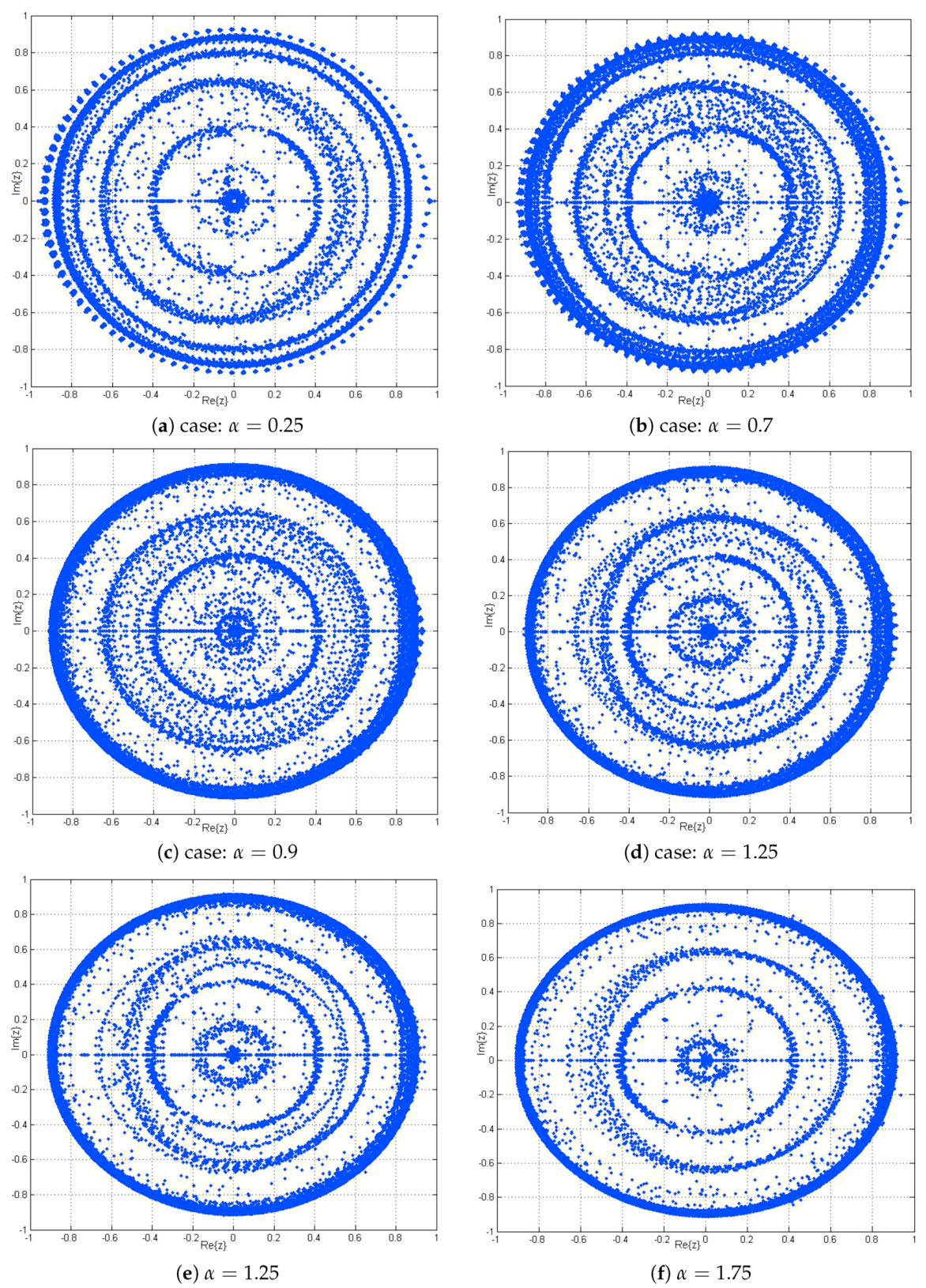
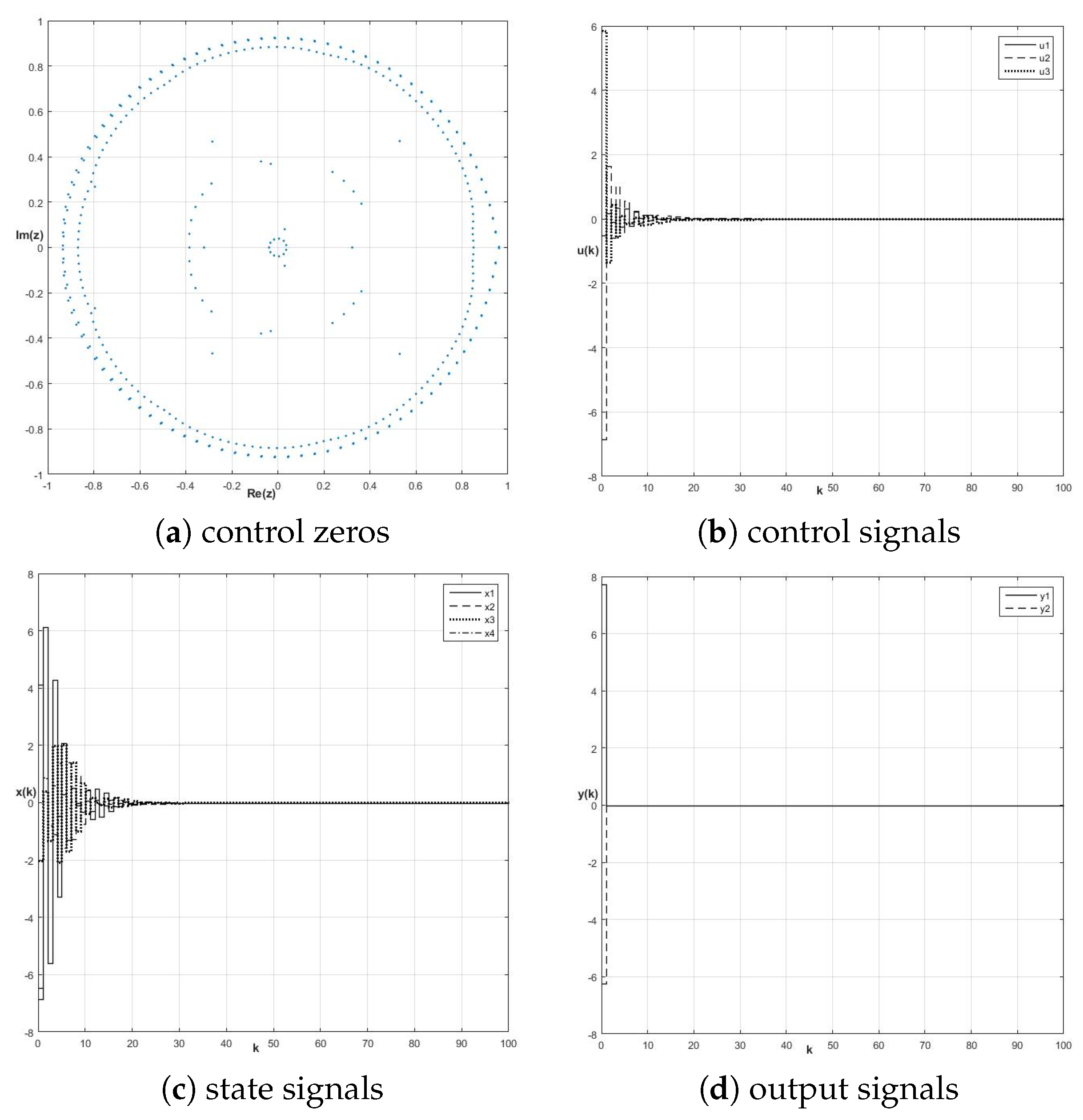
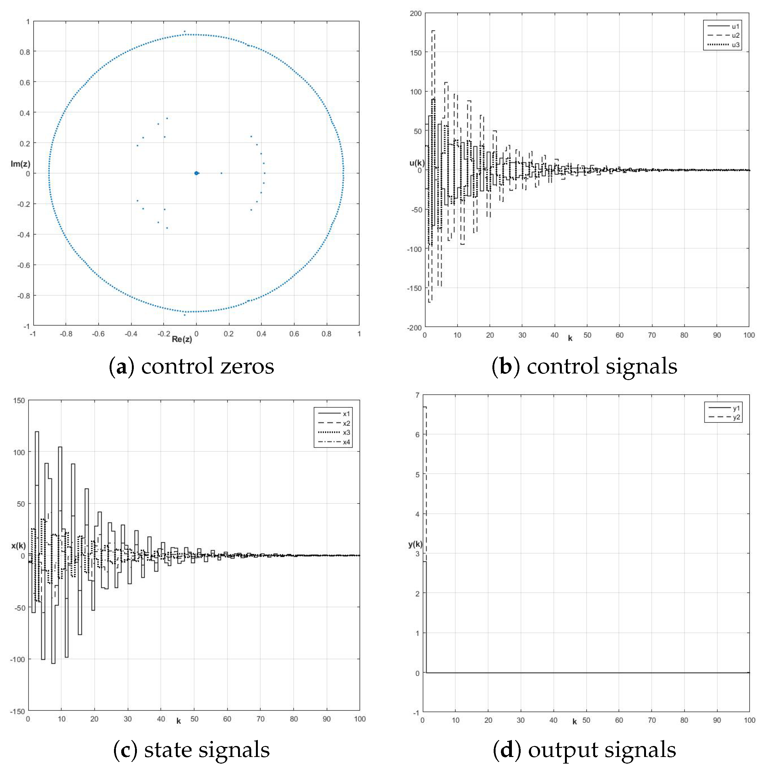
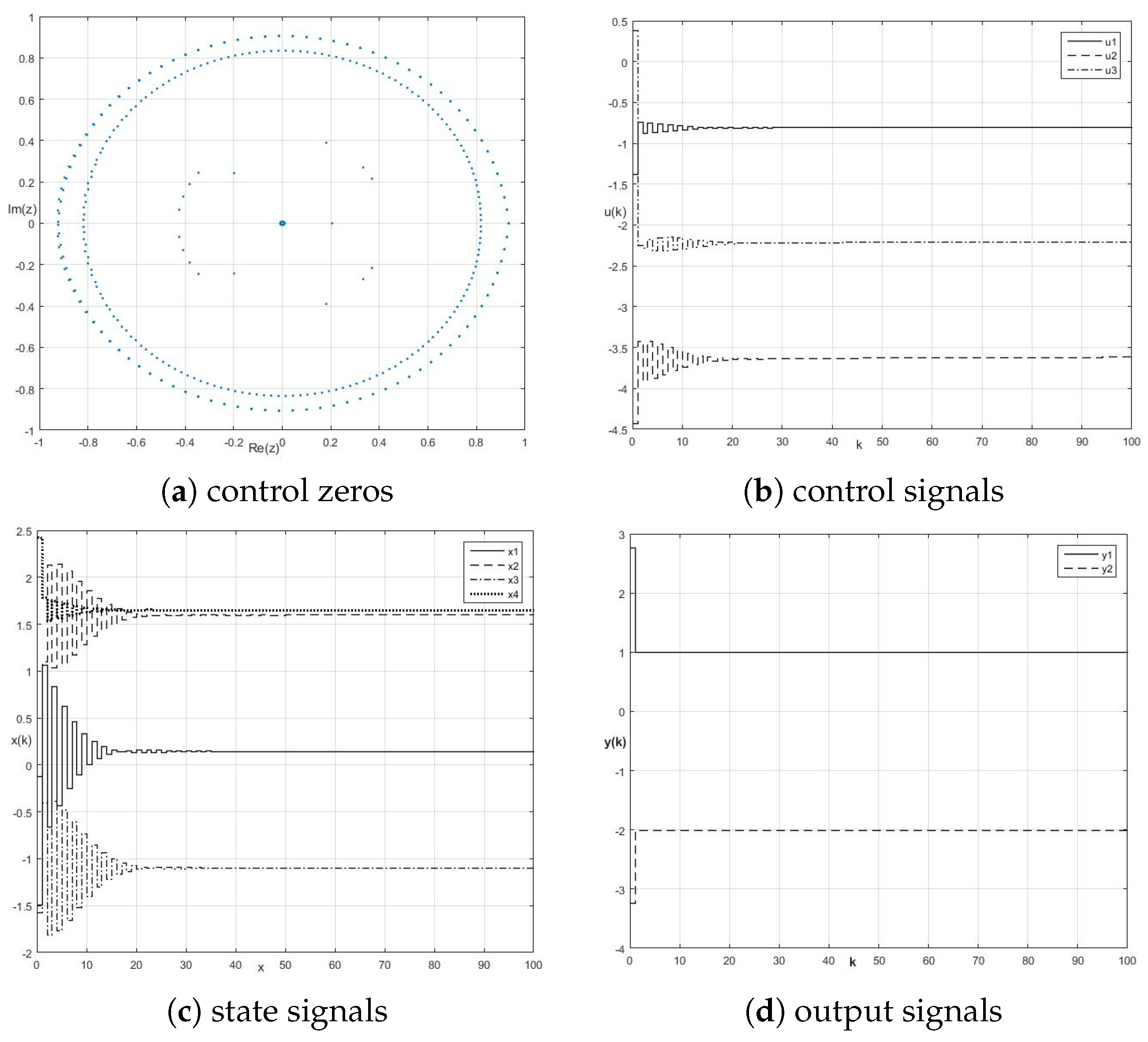
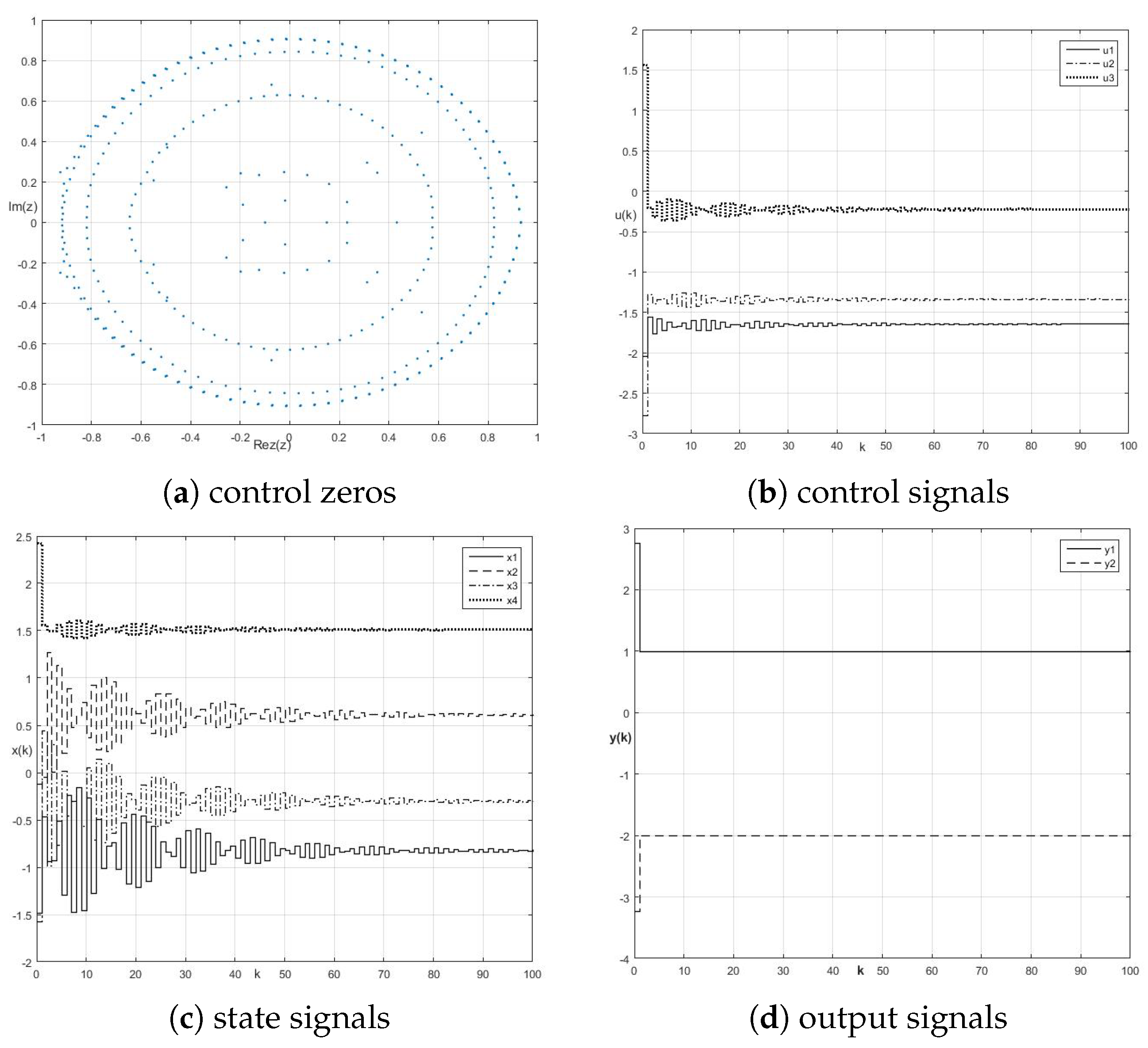
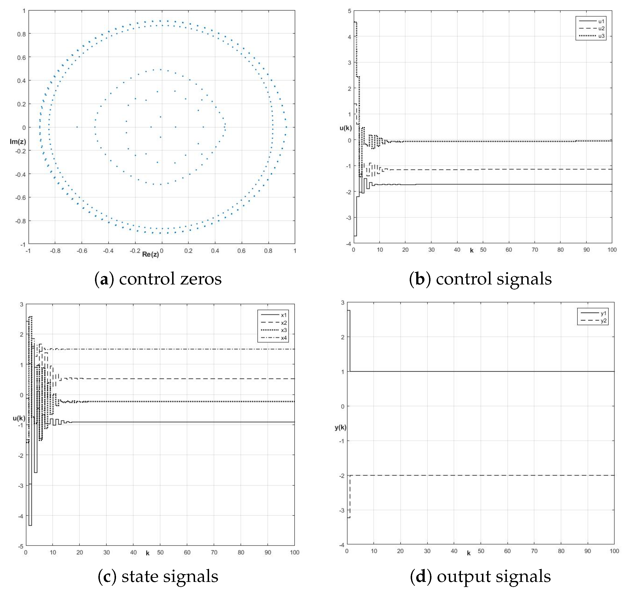
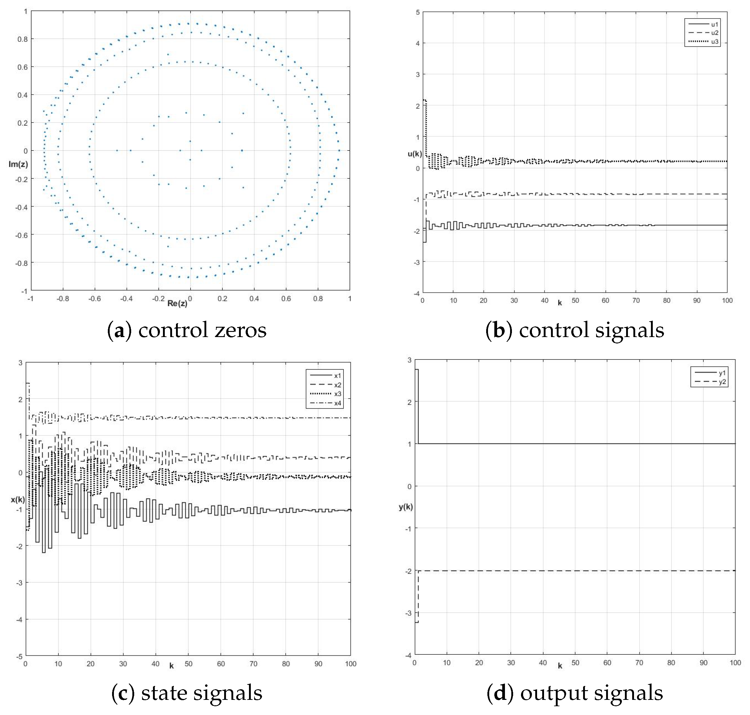
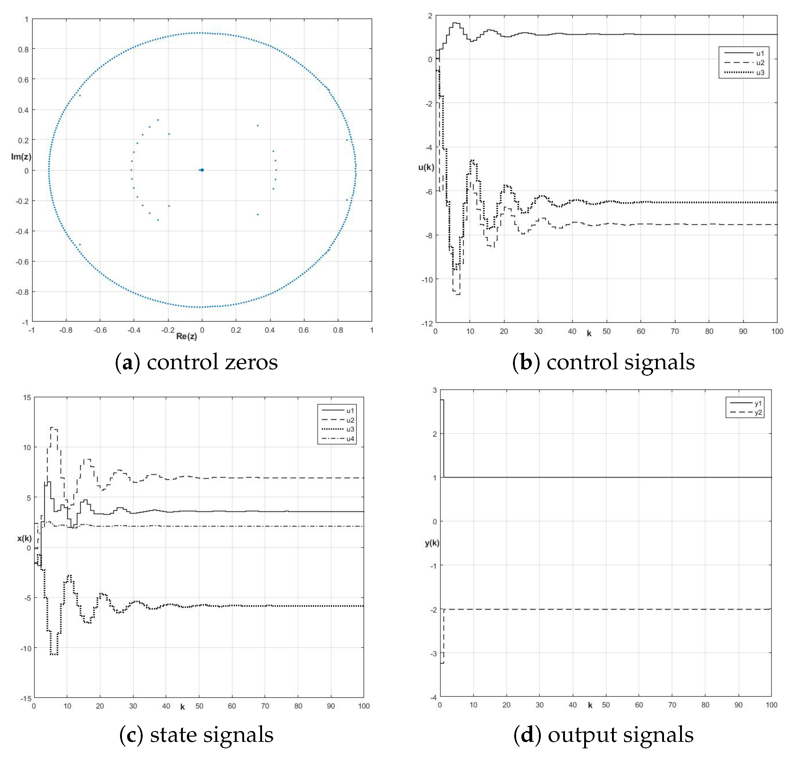
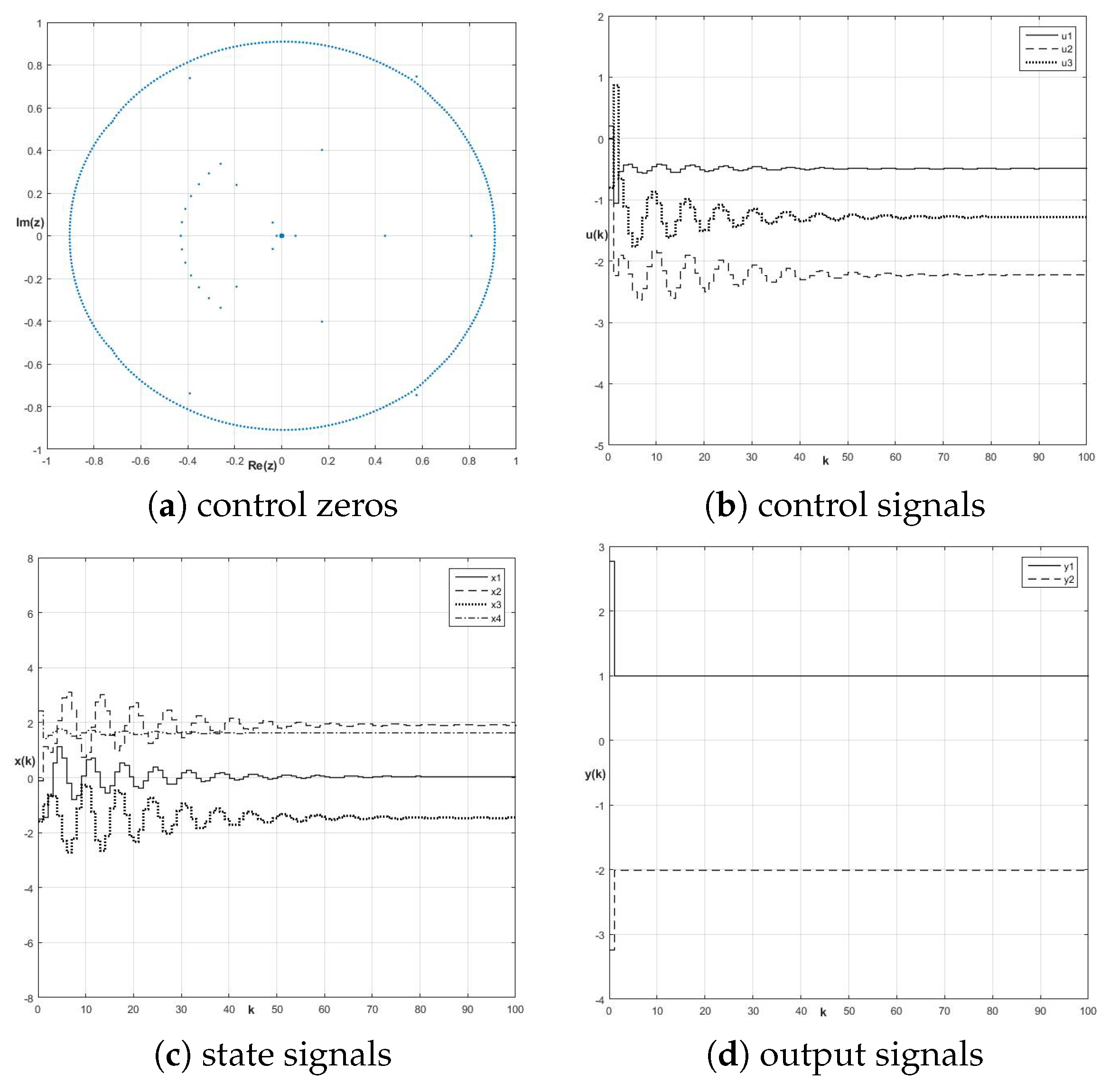
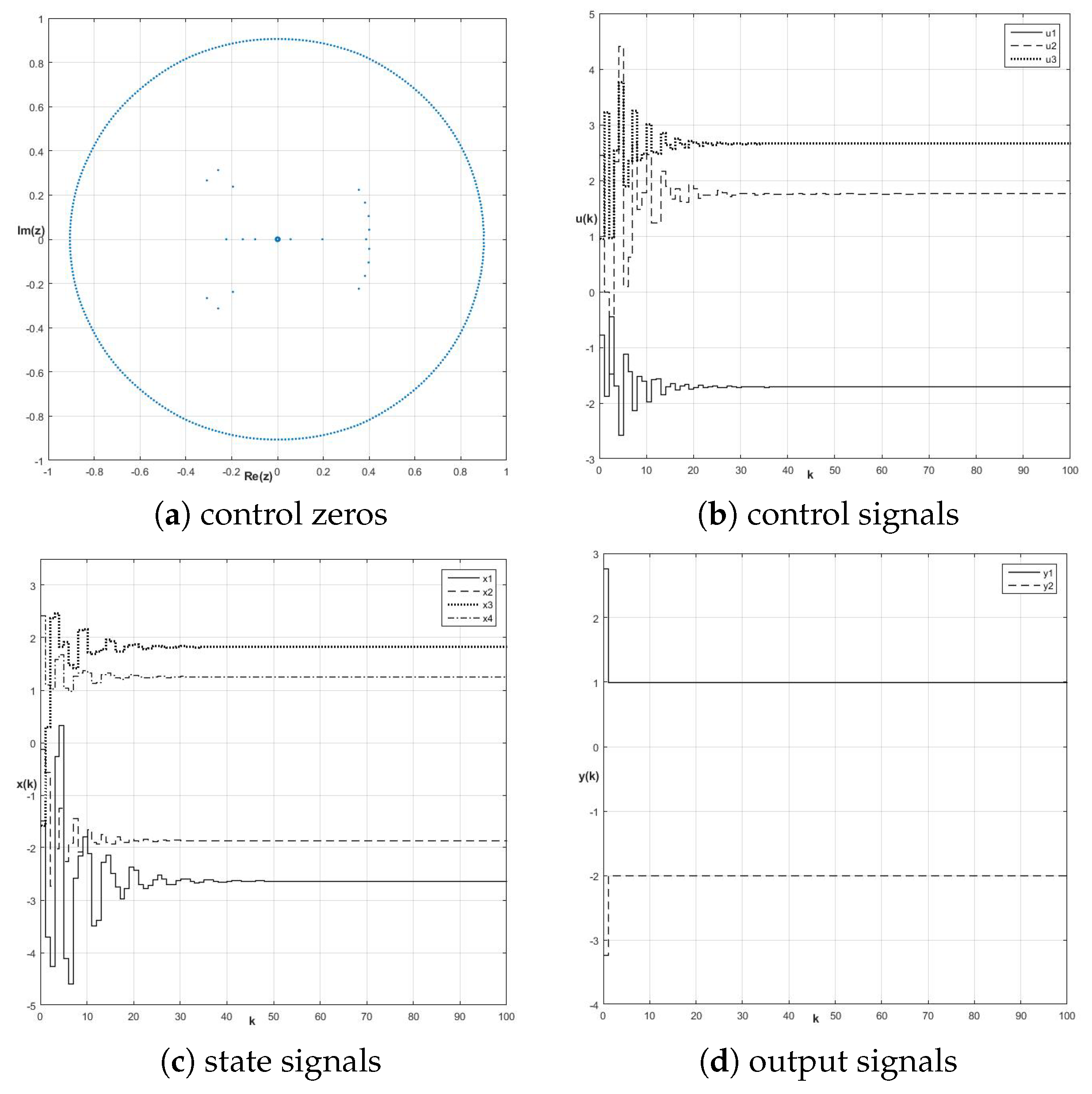
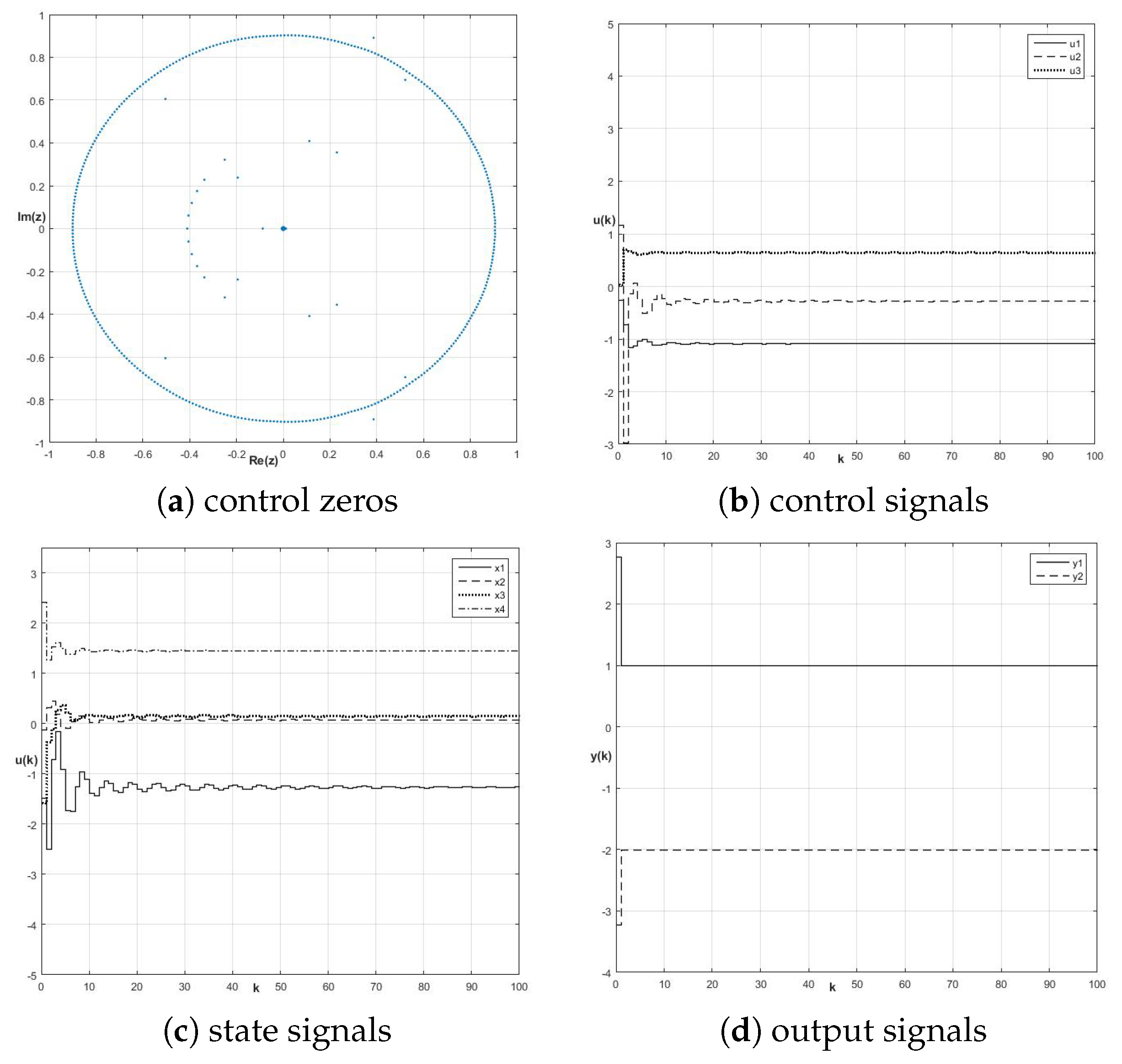
8.1. Control Zeros and Fractional-Order Perfect Control Stability

Consider the fractional-order system described by the G-L framework $S_{\mathrm{F}-\mathrm{O}}({\mathbf{A}}_{\mathbf{d}},\mathbf{B},\mathbf{C},\alpha )$ with three inputs and two outputs represented by the following initial matrices

$$\begin{array}{l}\hfill {\mathbf{A}}_{\mathbf{d}}=\left[\begin{array}{rrrr}\hfill 1.0074& 0.0904& 0.2564& -0.0390\\ \hfill 0.0112& -1.0188& 0.0722& 0.2614\\ \hfill -0.2558& -0.1174& -0.9684& -0.0172\\ \hfill 0.0995& -0.2274& 0.0924& -1.0378\end{array}\right],\\ \mathbf{B}=\left[\begin{array}{ccc}\hfill 1.2711& -0.4173& 0\\ \hfill -0.2963& -0.1041& -0.9926\\ \hfill 0& 0.5119& 0\\ \hfill -1.4916& -0.5796& -0.2039\end{array}\right],\\ \mathbf{C}=\left[\begin{array}{cccc}\hfill 0& -0.5355& -0.5290& 0.7724\\ \hfill 0.1737& 0& 0& -1.2248\end{array}\right],\\ {\mathbf{X}}_{\mathbf{0}}^{\mathbf{T}}=\left[\begin{array}{rrrr}-1.4851& -0.1159& -1.5747& 2.4256\end{array}\right].\end{array}$$

(35)

We assume that during the simulations, the matrices $\mathbf{B}$ and $\mathbf{C}$ are the subjects to change, to finally derive several various plants. For every pair $(\mathbf{B},\mathbf{C})$ the fractional-order perfect control schemes are established through an application of $\sigma$-inverse with arbitrary degrees of freedom $\beta$. Figure 1 presents the stability areas restricted by the sets of stable control zeros calculated according to the different operators $\alpha$. Every set of stable control zeros is obtained in the MATLAB/Simulink environment based on the stable fractional-order perfect control law. Naturally, the fractional-order perfect control systems prepared in Simulink have been supported by randomly chosen matrices $\mathbf{B}$, $\mathbf{C}$ and $\beta$ resulted from MATLAB script.

Figure 2 and Figure 3 show the stable fractional-order perfect control runs for initial plants $S({\mathbf{A}}_{\mathbf{d}},\mathbf{B},\mathbf{C},\alpha =0.75)$ and $S({\mathbf{A}}_{\mathbf{d}},\mathbf{B},\mathbf{C},\alpha =1.25)$ together with the respective stability areas.

8.2. Energy-Based Approach to Robustness of Fractional-Order Perfect Control

It is clear now that the proper selection of control zeros set affects the stability of the fractional-order perfect control algorithm. The second feature, strictly related to the control zeros, is robustness of such control strategy. In the next example this property is examined by a relatively simple simulation scenario. To show the fractional-order perfect control robustification the H-inverse, defined in Equation (13), and $\sigma$-inverse, given in Equation (10), are effectively employed as in Equations (16) and (15), respectively. This operation is essential in the cases where T-inverse (see Definition 1 and Equation (14)) is unstable.

Let us take into account the fractional-order system (35). After application of a right T-inverse we obtain unstable perfect control runs for chosen ${\alpha }_1=0.01$ and ${\alpha }_2=1.8$. However, for specific $\sigma$- and H-inverses, selected under optimization tasks in the MATLAB/Simulink environment, the control signal achieves the minimum-energy value according to the performance indices (33) or (34). Again, the fractional-order perfect control plants performed in Simulink have been assisted by degrees of freedom $\beta$ and $\mathbf{L}$ according to the MATLAB’s genetic algorithm mechanism. The results are piloted in Figure 4, Figure 5, Figure 6, Figure 7, Figure 8, Figure 9, Figure 10 and Figure 11.

9. Conclusions and Open Problems

The entire theory concerning the perfect control dedicated to multivariable fractional-order plants in the Grünwald–Letnikov state–space framework is presented in the paper. Due to the application of the newly introduced control zeros, associated with the discrete-time perfect control formula, the minimum/nonminimum-phase behavior of analyzed non-integer-order systems is defined. The results reported in this paper were confirmed by several simulation examples performed in the MATLAB/Simulink environment. The further research study can be focused on the implementation of the postulated ideas to cover the discrete-time minimum variance control algorithm. An extension of the introduced theory to the continuous-time fractional-order case is another open problem to be taken into account in the future research.

References

1. Latawiec, K.; Bańka, S.; Tokarzewski, J. Control zeros and nonminimum phase LTI MIMO systems. Annu. Rev. Control. 2000, 24, 105–112. [Google Scholar] [CrossRef]
2. Borisson, U. Self-tuning regulators for a class of multivariable systems. Automatica 1979, 15, 209–215. [Google Scholar] [CrossRef]
3. Åström, K.J. Introduction to Stochastic Control Theory; Academic Press: New York, NY, USA, 1970. [Google Scholar]
4. Åström, K.J.; Wittenmark, B. On self-tuning regulators. Automatica 1973, 9, 185–199. [Google Scholar] [CrossRef]
5. Ryan, E.P.; Sangwin, C.J.; Townsend, P. Controlled functional differential equations: Approximate and exact asymptotic tracking with prescribed transient performance. ESAIM COCV 2009, 15, 745–762. [Google Scholar] [CrossRef]
6. Hunek, W.P. Control Zeros for Continuous-Time LTI MIMO Systems and Their Application in the Theory of Circuits and Systems. Ph.D. Thesis, Opole University of Technology Press, Opole, Poland, 2003. [Google Scholar]
7. Dadhich, S.; Birk, W. Analysis and control of an extended Quadruple tank process. In Proceedings of the 13th IEEE European Control Conference (ECC’2014), Strasbourg, France, 24–27 June 2014; pp. 838–843. [Google Scholar] [CrossRef]
8. Hunek, W.P.; Latawiec, K. A study on new right/left inverses of nonsquare polynomial matrices. Int. J. Appl. Math. Comput. Sci. 2011, 21, 331–348. [Google Scholar] [CrossRef] [Green Version]
9. Lin, Z.; Saberi, A.; Sannuti, P.; Shamash, Y.A. Perfect regulation of linear discrete-time systems: A low-gain-based design approach. Automatica 1996, 32, 1085–1091. [Google Scholar] [CrossRef]
10. Zhang, T.; Li, H.G.; Zhong, Z.Y.; Cai, G.P. Hysteresis model and adaptive vibration suppression for a smart beam with time delay. J. Sound Vib. 2015, 358, 35–47. [Google Scholar] [CrossRef]
11. Zhang, T.; Yang, B.T.; Li, H.G.; Meng, G. Dynamic modeling and adaptive vibration control study for giant magnetostrictive actuators. Sens. Actuators A Phys. 2013, 190, 96–105. [Google Scholar] [CrossRef]
12. Tokarzewski, J. Zeros in Linear Systems: A Geometric Approach; Warsaw University of Technology Press: Warsaw, Poland, 2002. [Google Scholar]
13. Tokarzewski, J. A note on some characterization of invariant zeros in singular systems and algebraic criteria of nondegeneracy. Int. J. Appl. Math. Comput. Sci. 2004, 14, 149–159. [Google Scholar]
14. Tokarzewski, J. Finite Zeros in Discrete Time Control Systems; Lecture Notes in Control and Information Sciences; Springer: Berlin, Germany, 2006; Volume 338. [Google Scholar] [CrossRef]
15. Hunek, W.P.; Krok, M. Pole-free perfect control for nonsquare LTI discrete-time systems with two state variables. In Proceedings of the 2017 13th International Conference on Control & Automation (ICCA), Xi’an, China, 20–23 August 2017; pp. 329–334. [Google Scholar]
16. Nastac, S.; Debeleac, C.; Vlase, S. Hysteretically Symmetrical Evolution of Elastomers-Based Vibration Isolators within α-Fractional Nonlinear Computational Dynamics. Symmetry 2019, 11, 924. [Google Scholar] [CrossRef]
17. Jajarmi, A.; Hajipour, M.; Mohammadzadeh, E.; Baleanu, D. A new approach for the nonlinear fractional optimal control problems with external persistent disturbances. J. Frankl. Inst. 2018, 355, 3938–3967. [Google Scholar] [CrossRef]
18. Wei, Y.Q.; Liu, D.Y.; Boutat, D. Innovative fractional derivative estimation of the pseudo-state for a class of fractional order linear systems. Automatica 2019, 99, 157–166. [Google Scholar] [CrossRef]
19. Wach, Ł.; Hunek, W.P. Perfect control for fractional-order multivariable discrete-time systems. In Theoretical Developments and Applications of Non-Integer Order Systems; Springer: Cham, Switzerland, 2016; pp. 233–237. [Google Scholar]
20. Hunek, W.P. An application of new polynomial matrix σ-inverse in minimum-energy design of robust minimum variance control for nonsquare LTI MIMO systems. IFAC-PapersOnLine 2015, 48, 150–154. [Google Scholar] [CrossRef]
21. Hunek, W.P.; Krok, M. A study on a new criterion for minimum-energy perfect control in the state-space framework. Proc. Inst. Mech. Eng. Part I J. Syst. Control. Eng. 2019. [Google Scholar] [CrossRef]
22. Wang, G.; Wei, Y.; Qia, S. Generalized Inverses: Theory and Computations; Science Press: Beijing, China, 2018. [Google Scholar]
23. Wei, Y.; Stanimirović, P.S.; Petković, M.D. Numerical and Symbolic Computations of Generalized Inverses; World Scientific Publishing Co. Pte Ltd.: Singapore, 2018. [Google Scholar]
24. Hunek, W.P. New SVD-based matrix H-inverse vs. minimum-energy perfect control design for state-space LTI MIMO systems. In Proceedings of the 2016 20th International Conference on System Theory, Control and Computing (ICSTCC), Sinaia, Romania, 13–15 October 2016; pp. 14–19. [Google Scholar]
25. Noueili, L.; Chagra, W.; Ksouri, M. New Iterative Learning Control Algorithm Using Learning Gain Based on σ Inversion for Nonsquare Multi-Input Multi-Output Systems. Model. Simul. Eng. 2018, 2018, 4195938. [Google Scholar] [CrossRef]
26. Hunek, W.P.; Wach, Ł. Towards a New Stability Criterion for Fractional-Order Perfect Control of LTI MIMO Discrete-Time Systems in State Space. In Proceedings of the 2017 3rd IEEE International Conference on Cybernetics (CYBCONF), Exeter, UK, 21–23 June 2017; pp. 1–6. [Google Scholar]
27. De la Sen, M. On Cauchy’s Interlacing Theorem and the Stability of a Class of Linear Discrete Aggregation Models Under Eventual Linear Output Feedback Controls. Symmetry 2019, 11, 712. [Google Scholar] [CrossRef]
28. Ben-Israel, A.; Greville, T. Generalized Inverses, Theory and Applications, 2nd ed.; Springer: New York, NY, USA, 2003. [Google Scholar]
29. Bronnikov, A.; Borovkov, A. Inverse control of discrete-time multivariable systems. J. Frankl. Inst. 2002, 339, 335–345. [Google Scholar] [CrossRef]
30. Karampetakis, N.P.; Tzekis, P. On the computation of the generalized inverse of a polynomial matrix. IMA J. Math. Control Inf. 2001, 18, 83–97. [Google Scholar] [CrossRef]
31. Penrose, R. A generalized inverse for matrices. Math. Proc. Camb. Philos. Soc. 1955, 51, 406–413. [Google Scholar] [CrossRef] [Green Version]
32. Hunek, W.P.; Latawiec, K.; Stanisławski, R.; Łukaniszyn, M.; Dzierwa, P. A new form of a σ-inverse for nonsquare polynomial matrices. In Proceedings of the 2013 18th International Conference on Methods and Models in Automation and Robotics (MMAR), Miedzyzdroje, Poland, 26–29 August 2013; pp. 282–286. [Google Scholar]
33. Hunek, W.P.; Latawiec, K.J.; Majewski, P.; Dzierwa, P. An application of a new matrix inverse in stabilizing state-space perfect control of nonsquare LTI MIMO systems. In Proceedings of the 2014 19th International Conference on Methods and Models in Automation and Robotics (MMAR), Miedzyzdroje, Poland, 2–5 September 2013; pp. 451–455. [Google Scholar]
34. Majewski, P. Research towards Increasing the Capacity of Wireless Data Communication Using Inverses of Nonsquare Polynomial Matrices. Ph.D. Thesis, Opole University of Technology Press, Opole, Poland, 2017. [Google Scholar]
35. Dabiri, A.; Butcher, E.A.; Poursina, M.; Nazari, M. Optimal Periodic-Gain Fractional Delayed State Feedback Control for Linear Fractional Periodic Time-Delayed Systems. IEEE Trans. Autom. Control 2018, 63, 989–1002. [Google Scholar] [CrossRef]
36. Kaczorek, T. Minimum energy control of fractional descriptor positive discrete-time linear systems. Int. J. Appl. Math. Comput. Sci. 2014, 24, 735–743. [Google Scholar] [CrossRef] [Green Version]
37. Kaczorek, T. Minimum energy control of fractional positive continuous-time linear systems using Caputo-Fabrizio definition. Bull. Pol. Acad. Sci.-Tech. Sci. 2017, 65, 45–51. [Google Scholar] [CrossRef] [Green Version]
38. Klamka, J. Controllability and Minimum Energy Control Problem of Fractional Discrete-Time Systems. In New Trends in Nanotechology and Fractional Calculus Applications; Baleanu, D., Guvenc, Z.B., Machado, J.A.T., Eds.; Springer: Cham, The Netherlands, 2010; pp. 503–509. [Google Scholar] [CrossRef]
39. Merrikh-Bayat, F.; Karimi-Ghartemani, M. Method for designing PIλDμstabilisers for minimum-phase fractional-order systems. IET Control Theory Appl. 2010, 4, 61–70. [Google Scholar] [CrossRef]
40. Yige, Z.; Meirong, X. Stability and stabilization for a class of fractional-order linear time-delay systems. In Proceedings of the 2017 36th Chinese Control Conference (CCC), Dalian, China, 26–28 July 2017; pp. 11340–11344. [Google Scholar] [CrossRef]
41. Yuan, T.; Zheng, M.; Zhang, K.; Huang, T. Fractional-order PID controllers for stabilization of fractional-order time delay systems based on region stability. In Proceedings of the 2018 Chinese Control and Decision Conference (CCDC), Shenyang, China, 9–11 June 2018; pp. 6633–6638. [Google Scholar] [CrossRef]
Figure 1. Control zeros for fractional-order systems: time horizon k = 100 , y ref ( k + 1 ) = 0 (see Equation (24)).
Symmetry 11 01322 g001
Figure 2. Control zeros and time-domain signals, S ( A d , B , C , α = 0 . 25 ) , k = 100 , y ref ( k ) = 0 , T-inverse.
Symmetry 11 01322 g002
Figure 3. Control zeros and time-domain signals, S ( A d , B , C , α = 1 . 75 ) , k = 100 , y ref ( k ) = 0 , T-inverse.
Symmetry 11 01322 g003
Figure 4. Control zeros and time-domain signals, S ( A d , B , C , α = 0 . 01 ) , k = 100 , y ref ( k ) = 1 2 T , E 1 = 8 . 18 , E 2 = 1889 . 80 , stable H-inverse with L = 0 . 7231 1 . 7809 .
Symmetry 11 01322 g004
Figure 5. Control zeros and time-domain signals, S ( A d , B , C , α = 0 . 01 ) , k = 100 , y ref ( k ) = [ 1 2 ] , E 1 = 5 . 75 , E 2 = 468 . 81 , minimum-energy-based H-inverse with L = [ 10.1378 0.2495 ] .
Symmetry 11 01322 g005
Figure 6. Control zeros and time-domain signals, S ( A d , B , C , α = 0 . 01 ) , k = 100 , y ref ( k ) = 1 2 , E 1 = 44 . 92 , E 2 = 473 . 40 , stable σ -inverse with β = 1 . 0724 1 . 4588 0 . 9329 1 . 5464 0 . 6466 1 . 9729 .
Symmetry 11 01322 g006
Figure 7. Control zeros and time-domain signals, S ( A d , B , C , α = 0 . 01 ) , k = 100 , y ref ( k ) = 1 2 , E 1 = 6 . 21 , E 2 = 423 . 95 , minimum-energy-based σ -inverse with σ = 243 . 0453 73 . 0769 56 . 3869 890 . 1077 321 . 4291 1545 . 2586 .
Symmetry 11 01322 g007
Figure 8. Control zeros and time-domain signals, S ( A d , B , C , α = 1 . 80 ) , k = 100 , y ref ( k ) = [ 1 2 ] , E 1 = 216 . 13 , E 2 = 10117 . 60 , stable H-inverse with L = [ 1.8883 2.4348 ] .
Symmetry 11 01322 g008
Figure 9. Control zeros and time-domain signals, S ( A d , B , C , α = 1 . 80 ) , k = 100 , y ref ( k ) = [ 1 2 ] , E 2 = 680 . 61 , minimum-energy-based H-inverse with L = [ 0.7347 2.4624 ] .
Symmetry 11 01322 g009
Figure 10. Control zeros and time-domain signals, S ( A d , B , C , α = 1 . 80 ) , k = 100 , y ref ( k ) = 1 2 , E 1 = 40 . 56 , E 2 = 1335 . 14 , stable σ -inverse with β = 1 . 5432 0 . 7173 2 . 5449 1 . 5224 0 . 4069 2 . 6763 .
Symmetry 11 01322 g010
Figure 11. Control zeros and time-domain signals, S ( A d , B , C , α = 1 . 80 ) , k = 100 , y ref ( k ) = 1 2 , E 1 = 10 . 88 , E 2 = 176 . 35 , minimum-energy-based σ -inverse with β = 2 . 5685 0 . 9337 1 . 3965 1 . 7471 0 . 3845 1 . 0463 .
Symmetry 11 01322 g011