Lie Symmetries, Conservation Laws and Exact Solutions for Jaulent-Miodek Equations

Abstract

In this paper, the Lie symmetries of the Jaulent-Miodek (JM) equations are calculated and one dimensional optimal systems of Lie algebra are obtained. Furthermore, the conservation laws are constructed by using the adjoint equation method. Finally, the exact solutions of the equations are obtained by the conservation laws.

1. Introduction

In this paper, we consider the Jaulent-Miodek (JM) equations [1]

$$\left\{\begin{array}{c}{u}_t+u_{xxx}+\frac{3}{2}v{v}_{xxx}+\frac{9}{2}{v}_x{v}_{xx}-6u{u}_x-6uv{v}_x-\frac{3}{2}{u}_x{v}^2=0,\hfill \\ v_t+v_{xxx}-6u_{x}v-6u{v}_x-\frac{15}{2}{v}_x{v}^2=0.\hfill \end{array}\right.$$

(1)

which associates with the JM spectral problem [2,3] and energy-dependent Schrodinger potential [4,5,6]. There are a plethora of methods to solve system (1), such as exp-function method [7,8,9,10], tanh-coth and sech methods [11,12,13,14]. A numerical method is available in [15]. According to our understanding, the Lie symmetry and conservation laws of the JM equations have not been done yet. This paper will give the symmetry reduction and conservation laws of the system (1) and construct its exact solution.

The structure of this paper is as follows: In Section 2, the Lie symmetry of the Jaulent-Miodek (JM) equations are calculated and one dimensional optimal systems of Lie algebra are obtained; in Section 3, the conservation laws of the system are given by adjoint equation method; in Section 4, the exact solutions of the system are constructed by the conservation laws; and in Section 5, a brief summary is made of the full text.

2. Lie Symmetry Analysis and Optimal Systems

2.1. Lie Symmetry

In this section, we will perform Lie symmetry analysis for the system (1). We first assume that the infinitesimal generator [16] allowed of the system (1) is:

$$V={\xi }^1(t,x,u,v)\frac{\partial }{\partial t}+{\xi }^2(t,x,u,v)\frac{\partial }{\partial x}+{\eta }^1(t,x,u,v)\frac{\partial }{\partial u}+{\eta }^2(t,x,u,v)\frac{\partial }{\partial v},$$

(2)

where ${\xi }^1(t,x,u,v),{\xi }^2(t,x,u,v),{\eta }^1(t,x,u,v),{\eta }^2(t,x,u,v)$ are coefficient functions to be determined.

For the system (1), V satisfies the following Lie symmetry conditions as follows

$$\begin{array}{cc}\hfill P{r}^{3}V({\Delta }_1){|}_{{\Delta }_1=0,{\Delta }_2=0}& =0,\hfill \\ \hfill P{r}^{3}V({\Delta }_2){|}_{{\Delta }_1=0,{\Delta }_2=0}& =0,\hfill \end{array}$$

(3)

where

$$\begin{array}{cc}\hfill {\Delta }_1& =u_t+u_{xxx}+\frac{3}{2}v{v}_{xxx}+\frac{9}{2}{v}_x{v}_{xx}-6u{u}_x-6uv{v}_x-\frac{3}{2}{u}_x{v}^2,\hfill \\ \hfill {\Delta }_2& =v_t+v_{xxx}-6u_{x}v-6u{v}_x-\frac{15}{2}{v}_x{v}^2.\hfill \end{array}$$

(4)

By Lie’s theory, the third prolongation [17] of (2) is of the form

$$\begin{array}{c}\hfill \begin{array}{cc}\hfill P{r}^{(3)}V& =V+{\eta }^{1x}\frac{\partial }{\partial u_x}+{\eta }^{1t}\frac{\partial }{\partial u_t}+{\eta }^{2x}\frac{\partial }{\partial v_x}+{\eta }^{2t}\frac{\partial }{\partial v_t}+{\eta }^{1xx}\frac{\partial }{\partial u_{xx}}+{\eta }^{1xt}\frac{\partial }{\partial u_{xt}}+{\eta }^{1tt}\frac{\partial }{\partial u_{tt}}\hfill \\ \hfill & +{\eta }^{2xx}\frac{\partial }{\partial v_{xx}}+{\eta }^{2xt}\frac{\partial }{\partial v_{xt}}+{\eta }^{2tt}\frac{\partial }{\partial v_{tt}}+{\eta }^{1xxx}\frac{\partial }{\partial u_{xxx}}+{\eta }^{1xxt}\frac{\partial }{\partial u_{xxt}}+{\eta }^{1xtt}\frac{\partial }{\partial u_{xtt}}\hfill \\ \hfill & +{\eta }^{1ttt}\frac{\partial }{\partial u_{ttt}}+{\eta }^{2xxx}\frac{\partial }{\partial v_{xxx}}+{\eta }^{2xxt}\frac{\partial }{\partial v_{xxt}}+{\eta }^{2xtt}\frac{\partial }{\partial v_{xtt}}+{\eta }^{2ttt}\frac{\partial }{\partial v_{ttt}},\hfill \end{array}\end{array}$$

(5)

where

$$\begin{array}{c}\hfill \begin{array}{cc}\hfill & {\eta }^{1x}=D_x({\eta }^1-{\xi }^1{u}_t-{\xi }^2{u}_x)+{\xi }^1{u}_{tx}+{\xi }^2{u}_{xx},\hfill \\ \hfill & {\eta }^{1t}=D_t({\eta }^1-{\xi }^1{u}_t-{\xi }^2{u}_x)+{\xi }^1{u}_{tt}+{\xi }^2{u}_{xt},\hfill \\ \hfill & {\eta }^{2x}=D_x({\eta }^2-{\xi }^1{v}_t-{\xi }^2{v}_x)+{\xi }^1{v}_{tx}+{\xi }^2{v}_{xx},\hfill \\ \hfill & {\eta }^{2t}=D_t({\eta }^2-{\xi }^1{v}_t-{\xi }^2{v}_x)+{\xi }^1{v}_{tt}+{\xi }^2{v}_{xt},\hfill \\ \hfill & {\eta }^{1xx}=D_{xx}({\eta }^1-{\xi }^1{u}_t-{\xi }^2{u}_x)+{\xi }^1{u}_{txx}+{\xi }^2{u}_{xxx},\hfill \\ \hfill & {\eta }^{2xx}=D_{xx}({\eta }^2-{\xi }^1{v}_t-{\xi }^2{v}_x)+{\xi }^1{v}_{txx}+{\xi }^2{v}_{xxx},\hfill \\ \hfill & {\eta }^{1xxx}=D_{xxx}({\eta }^1-{\xi }^1{u}_t-{\xi }^2{u}_x)+{\xi }^1{u}_{txxx}+{\xi }^2{u}_{xxxx},\hfill \\ \hfill & {\eta }^{2xxx}=D_{xxx}({\eta }^2-{\xi }^1{v}_t-{\xi }^2{v}_x)+{\xi }^1{v}_{txxx}+{\xi }^2{v}_{xxxx}.\hfill \end{array}\end{array}$$

(6)

Combining (3) and (4), we get the determining equations of system (1) as follows:

$$\left\{\begin{array}{cc}\hfill & {\eta }^1(-6u_x-6v{v}_x)+{\eta }^2(\frac{3}{2}{v}_{xxx}-6u{v}_x-3u_{x}v)+{\eta }^{1x}(-6u-\frac{3}{2}{v}^2)+{\eta }^{1t}\hfill \\ \hfill & +{\eta }^{2x}(\frac{9}{2}{v}_{xx}-6uv)+{\eta }^{2xx}\frac{9}{2}{v}_x+{\eta }^{1xxx}+{\eta }^{2xxx}\frac{3}{2}v=0,\hfill \\ \hfill & {\eta }^1(-6v_x)+{\eta }^2(-6u_x-15v_{x}v)+{\eta }^{1x}(-6v)+{\eta }^{2x}(-6u-\frac{15}{2}{v}^2)+{\eta }^{2t}+{\eta }^{2xxx}=0.\hfill \end{array}\right.$$

(7)

Substituting system (6) into the equivalent condition (7), and making the coefficients of the various monomials in partial derivatives with respect to x and various powers of u equaled, one then obtains the over determining equations of system (7):

$$\begin{array}{cccc}\begin{array}{l}{\xi }_u^1=0,\\ {\xi }_v^1=0,\\ {\xi }_x^1=0,\\ 3{\eta }^1+2u{\xi }_t^1=0,\end{array}\hfill & \begin{array}{l}{\xi }_u^2=0,\\ {\xi }_v^2=0,\\ {\xi }_t^2=0,\\ {\eta }^1+2u{\xi }_x^2=0,\end{array}\hfill & \begin{array}{l}{\eta }_v^1=0,\\ {\eta }_t^1=0,\\ {\eta }_x^1=0,\\ {\eta }^1-u{\eta }_u^1=0.\end{array}\hfill & \begin{array}{l}v{\eta }^1-2u{\eta }^2=0,\\ \hspace{1em}\\ \hspace{1em}\\ \hspace{1em}\end{array}\hfill \end{array}$$

(8)

Solving (8), one can get

$$\begin{array}{ll}\begin{array}{l}{\xi }^1=-\frac{3}{2}{c}_{3}t+c_1,\\ {\eta }^1=c_{3}u,\end{array}\hfill & \begin{array}{l}{\xi }^2=-\frac{c_3}{2}x+c_2,\\ {\eta }^2=\frac{c_3}{2}v.\end{array}\hfill \end{array}$$

(9)

where $c_1,c_2,c_3$ are three arbitrary constants. Therefore, the three-dimensional Lie algebra of infinitesimal symmetries for Jaulent-Miodek (JM) equations (1) are spanned by the following three vector fields:

$$\begin{array}{c}\hfill \begin{array}{cc}\hfill & V_1=\frac{\partial }{\partial t},\hfill \\ \hfill & V_2=\frac{\partial }{\partial x},\hfill \\ \hfill & V_3=-\frac{3}{2}t\frac{\partial }{\partial x}-\frac{1}{2}x\frac{\partial }{\partial t}+u\frac{\partial }{\partial u}+\frac{1}{2}v\frac{\partial }{\partial v}.\hfill \end{array}\end{array}$$

(10)

2.2. Optimal System

In this section, we research the one-dimensional optimal system of (10). The basic method of constructing one-dimensional optimal system is given in ref. [18]. The adjoint transformation is expressed as the following series form:

$$Ad(e^{ϵV_i})V_j=V_j-ϵ[V_i,V_j]+\frac{1}{2}{ϵ}^2[V_i,[V_i,V_j]]-\dots ,$$

where $ϵ$ is a parameter. $[V_i,V_j]$ is the usual commutator and the calculation formula is as follows:

$$[V_i,V_j]=V_i{V}_j-V_j{V}_i.$$

Hence we have the following commutator table [19] (See

Table 1. Commutator table of the Lie algebra.

$[V_i,V_j]$	$V_1$	$V_2$	$V_3$
$V_1$	0	0	$-\frac{3}{2}{V}_1$
$V_2$	0	0	$-\frac{1}{2}{V}_2$
$V_3$	$\frac{3}{2}{V}_1$	$\frac{1}{2}{V}_2$	0

) and the adjoint table (See

Table 2. Adjoint table of the Lie algebra.

$Ad$	$V_1$	$V_2$	$V_3$
$V_1$	$V_1$	$V_2$	$V_3+\frac{3}{2}ϵV_1$
$V_2$	$V_1$	$V_2$	$V_3+\frac{1}{2}ϵV_2$
$V_3$	$e^{-\frac{3}{2}ϵ}{V}_1$	$e^{-\frac{1}{2}ϵ}{V}_2$	$V_3$

).

Next, according to the method of constructing one dimensional optimal system in [18], we set up the following non-zero vector field with arbitrary coefficients $a_1,a_2,a_3$

$$V=a_1{V}_1+a_2{V}_2+a_3{V}_3.$$

Step 1:

Without loss of generality, supposing that $a_3\ne 0$ and setting $a_3=1$, then the vector V becomes

$$V=a_1{V}_1+a_2{V}_2+V_3.$$

To eliminate the coefficient of $V_1$, using $Ad(e^{ϵV_1})$ to act on above V, we gain

$$V^{\prime }=Ad(e^{ϵV_1})V=a_1{V}_1+a_2{V}_2+V_3+\frac{3}{2}ϵV_1=(a_1+\frac{3}{2}ϵ)V_1+a_2{V}_2+V_3,$$

where the group parameter $ϵ=-\frac{2a_1}{3}$. Therefore, $V^{\prime }=a_2{V}_2+V_3.$ We continue to eliminate $V_2$, using $Ad(e^{ϵV_2})$ to act on above $V^{\prime }$, we derive

$$V^{″}=Ad(e^{ϵV_2})V^{\prime }=a_2{V}_2+V_3+\frac{1}{2}{V}_2=(a_2+\frac{1}{2}ϵ)V_2+V_3,$$

where the group parameter $ϵ=-2a_2$. Therefore, $V^{″}=V_3$.

Step 2:

Supposing that $a_3=0,a_2\ne 0$ and setting $a_2=1$, then the vector V prove to be

$$V=a_1{V}_1+V_2.$$

Based on the above method, we know that neither $V_1$ and $V_2$ can be eliminated.

Step 3:

Supposing that $a_3=0,a_2=0,a_1\ne 0$ and setting $a_1=1$, then the vector V turn into

$$V=V_1.$$

Based on the adjoint representations of the vector field, we obtain the optimal systems of Lie algebra.

$$[V_1,V_3,a{V}_1+V_2],$$

with a is an arbitrary constant.

For $V_1$, the system of (1) is reduced as follows:

$$\left\{\begin{array}{c}{F}^{‴}+\frac{3}{2}H{H}^{‴}+\frac{9}{2}{H}^{\prime }{H}^{″}-6F{F}^{\prime }-6FH{H}^{\prime }-\frac{3}{2}{F}^{\prime }{H}^2=0,\hfill \\ H^{‴}-6F^{\prime }H-6F{H}^{\prime }-\frac{15}{2}{H}^{\prime }{H}^2=0,\hfill \end{array}\right.$$

(11)

where, $u(x,t)=F(\xi ),v(x,t)=H(\xi ),\xi =x$.

For $a{V}_1+V_2$, the system of (1) is reduced as follows:

$$\left\{\begin{array}{c}{F}^{\prime }-a^3{F}^{‴}-\frac{3a^3}{2}H{H}^{‴}-\frac{9a^3}{2}{H}^{\prime }{H}^{″}+6aF{F}^{\prime }+6aFH{H}^{\prime }-\frac{3a}{2}{F}^{\prime }{H}^2=0,\hfill \\ H^{\prime }-a^3{H}^{‴}+6a{F}^{\prime }H+6aF{H}^{\prime }+\frac{15a}{2}{H}^{\prime }{H}^2=0,\hfill \end{array}\right.$$

(12)

where, $u(x,t)=F(\xi ),v(x,t)=H(\xi ),\xi =t-ax$.

Obviously, Both (11) and (12) are difficult to calculate, So we take the following method to solve the system (1).

3. The Conservation Laws of Jaulennt-Miodek Equations

In this section, we construct the conservation laws by using the adjoint equations method [20,21,22,23,24].

3.1. Adjoint Equations and Lagrange Functions

The formal Lagrangian for the system (1) is given by

$$\begin{array}{c}\hfill \begin{array}{cc}\hfill & L={\theta }_1(u_t+u_{xxx}+\frac{3}{2}v{v}_{xxx}+\frac{9}{2}{v}_x{v}_{xx}-6u{u}_x-6uv{v}_x-\frac{3}{2}{u}_x{v}^2)+\hfill \\ \hfill & {\theta }_2(v_t+v_{xxx}-6u_{x}v-6u{v}_x-\frac{15}{2}{v}_x{v}^2),\hfill \end{array}\end{array}$$

(13)

where ${\theta }_1$ and ${\theta }_2$ are new dependent variables of $t,x,u,v$. The adjoint system for the Equation (1) is defined as

$$\begin{array}{c}\hfill \begin{array}{cccc}\hfill & \frac{\delta L}{\delta u}=0,\hfill & & \frac{\delta L}{\delta v}=0,\end{array}\end{array}$$

where

$$\begin{array}{c}\hfill \begin{array}{cc}\hfill & \frac{\delta L}{\delta u}=\frac{\partial L}{\partial u}-D_t\frac{\partial L}{\partial u_t}-D_x\frac{\partial L}{\partial u_x}+D_t{D}_t\frac{\partial L}{\partial u_{tt}}+D_t{D}_x\frac{\partial L}{\partial u_{tx}}+D_x{D}_x\frac{\partial L}{\partial u_{xx}}-D_t{D}_t{D}_t\frac{\partial L}{\partial u_{ttt}}\hfill \\ \hfill & -D_t{D}_x{D}_x\frac{\partial L}{\partial u_{txx}}-D_t{D}_t{D}_x\frac{\partial L}{\partial u_{ttx}}-D_x{D}_x{D}_x\frac{\partial L}{\partial u_{xxx}}+\dots ,\hfill \\ \hfill & \frac{\delta L}{\delta v}=\frac{\partial L}{\partial v}-D_t\frac{\partial L}{\partial v_t}-D_x\frac{\partial L}{\partial v_x}+D_t{D}_t\frac{\partial L}{\partial v_{tt}}+D_t{D}_x\frac{\partial L}{\partial v_{tx}}+D_x{D}_x\frac{\partial L}{\partial v_{xx}}-D_t{D}_t{D}_t\frac{\partial L}{\partial v_{ttt}}\hfill \\ \hfill & -D_t{D}_x{D}_x\frac{\partial L}{\partial v_{txx}}-D_t{D}_t{D}_x\frac{\partial L}{\partial v_{ttx}}-D_x{D}_x{D}_x\frac{\partial L}{\partial v_{xxx}}+\dots .\hfill \end{array}\end{array}$$

(14)

For system (1), The adjoint equations have the following form

$$\left\{\begin{array}{c}{F}_1=\frac{\delta L}{\delta u}=-3{\theta }_{1}v{v}_x+6{\theta }_{1x}u+\frac{3}{2}{\theta }_{1x}{v}^2+6{\theta }_{2x}v-{\theta }_{1xxx}-{\theta }_{1t}=0,\hfill \\ F_2=\frac{\delta L}{\delta v}=3{\theta }_{1}v{u}_x-\frac{9}{2}{\theta }_{1x}{v}_{xx}+6{\theta }_{1x}uv+6{\theta }_{2x}u+\frac{15}{2}{\theta }_{2x}{v}^2-\frac{3}{2}{\theta }_{1xxx}v-{\theta }_{2t}-{\theta }_{2xxx}=0,\hfill \end{array}\right.$$

(15)

where, the solution to system (15) can be ${\theta }_1=2$, ${\theta }_2=v$. So we derive the Lagrangian

$$\begin{array}{c}\hfill \begin{array}{cc}\hfill & L=2(u_t+u_{xxx}+\frac{3}{2}v{v}_{xxx}+\frac{9}{2}{v}_x{v}_{xx}-6u{u}_x-6uv{v}_x-\frac{3}{2}{u}_x{v}^2)+\hfill \\ \hfill & v(v_t+v_{xxx}-6u_{x}v-6u{v}_x-\frac{15}{2}{v}_x{v}^2)\hfill \end{array}\end{array}$$

(16)

3.2. Conservation Laws

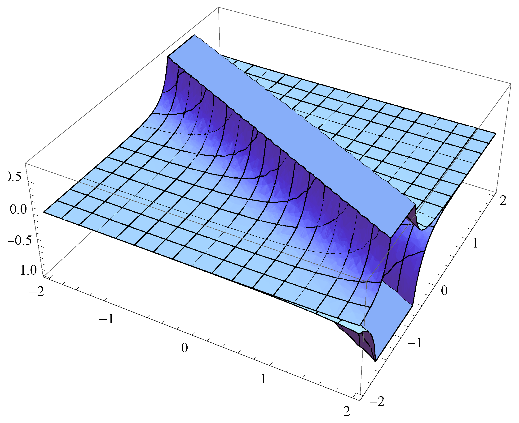
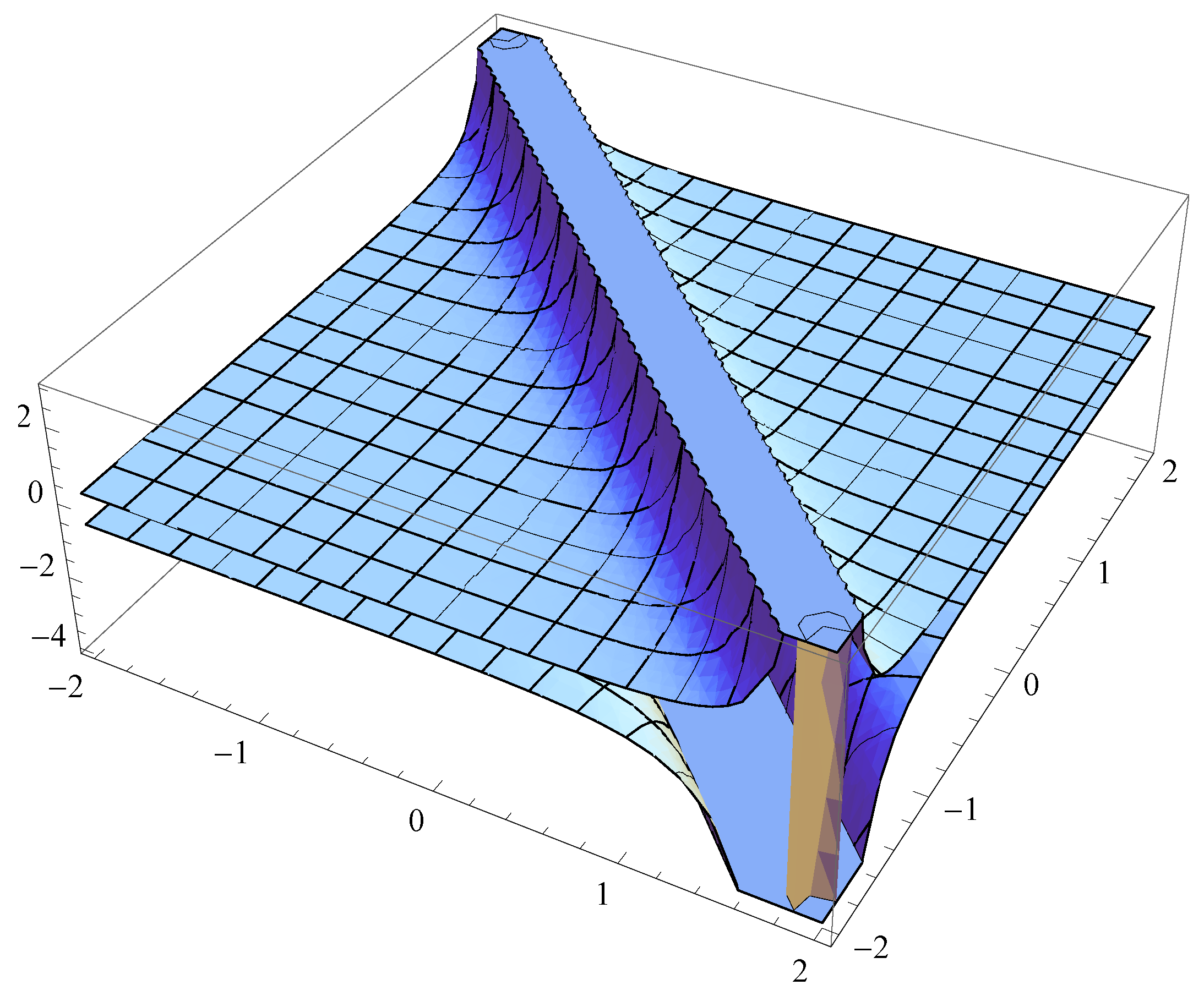
Every Lie symmetry provides a conservation law for system (1). The elements of the conservation vector $(C^1,C^2)$ are defined by the following expression:

$$\begin{array}{c}\hfill \begin{array}{cc}\hfill & C^i={\xi }^{i}L+W^{\alpha }[\frac{\partial L}{\partial u_i^{\alpha }}-D_j\frac{\partial L}{\partial u_{ij}^{\alpha }}+D_j{D}_k\frac{\partial L}{\partial u_{ijk}^{\alpha }}+\dots ]+D_j(W^{\alpha })[\frac{\partial L}{\partial u_{ij}^{\alpha }}-D_k\frac{\partial L}{\partial u_{ijk}^{\alpha }}+\dots ]\hfill \\ \hfill & +D_j{D}_k(W^{\alpha })[\frac{\partial L}{\partial u_{ijk}^{\alpha }}+\dots ]+\dots ,\hfill \end{array}\end{array}$$

(17)

where, $W^{\alpha }={\eta }^{\alpha }-{\xi }^j{u}_j^{\alpha }.$ Hence, the conservation laws for system (1) are given by

$$\begin{array}{cccc}\hfill & D_i(C^i){|}_{(1.1)}=0,\hfill & \hfill & i=1,2.\hfill \end{array}$$

Next we consider conservation laws in three cases.

Case 1. 

For$V_1=\frac{\partial }{\partial t}$, we obtain

$$\begin{array}{ccc}\hfill & W^1=-u_t,\hfill & \hfill W^2=-v_t.\end{array}$$

The conservation law of system (1) is

$$\begin{array}{cc}\hfill & D_t(-2u_t-v{v}_t)+D_x(12u{u}_t+9v^2{u}_t-2u_{txx}-4v_t{v}_{xx}+18uv{v}_t+\frac{15}{2}{v}^3{v}_t-5v_{tx}{v}_x-4v{v}_{txx})=0.\hfill \end{array}$$

Case 2. 

For $V_2=\frac{\partial }{\partial x}$, we derive

$$\begin{array}{cccc}\hfill & W^1=-u_x,\hfill & \hfill & W^2=-v_x.\hfill \end{array}$$

The conservation law of system (1) is

$$\begin{array}{cc}\hfill & D_t(-2u_x-v{v}_x)+D_x(2u_t+v{v}_t)=0.\hfill \end{array}$$

Case 3. 

For $V_3=-\frac{3}{2}t\frac{\partial }{\partial t}-\frac{1}{2}x\frac{\partial }{\partial x}+\frac{\partial }{\partial u}+\frac{1}{2}v\frac{\partial }{\partial v}$, We have

$$\begin{array}{cccc}\hfill & W^1=u+\frac{3}{2}t{u}_t+\frac{1}{2}x{u}_x,\hfill & \hfill & W^2=\frac{1}{2}v+\frac{3}{2}t{v}_t+\frac{1}{2}x{v}_x.\hfill \end{array}$$

The conservation law of system (1) is

$$\begin{array}{c}\hfill \begin{array}{c}{D}_t(2u+3t{u}_t+x{u}_x+\frac{1}{2}{v}^2+\frac{3}{2}tv{v}_t+\frac{1}{2}xv{v}_x)+D_x(-12u^2-18tu{u}_t-6xu{u}_x-18u{v}^2-\frac{27}{2}t{v}^2{u}_t\hfill \\ -\frac{9}{2}x{v}^2{u}_x+3t{u}_{txx}+4u_{xx}+x{u}_{xxx}+8v{v}_{xx}+6t{v}_t{v}_{xx}+\frac{9}{2}x{v}_x{v}_{xx}-27tuv{v}_t-9xuv{v}_x-\frac{15}{4}{v}^4-\hfill \\ \frac{45}{4}t{v}^3{v}_t-\frac{15}{4}x{v}^3{v}_x+5v_x^2+\frac{27}{2}tv{v}_{txx}+2x{v}_{xxx})=0.\hfill \end{array}\end{array}$$

4. Exact Solutions

In this section, we consider the exact solutions [25,26,27,28,29] by using the method of conservation laws.

For the conservation law of $V_2$, from (Section 3.2), we obtain the conservation law of $V_2$

$$\begin{array}{cc}\hfill & D_t(-2u_x-v{v}_x)+D_x(2u_t+v{v}_t)=0.\hfill \end{array}$$

Let

$$\begin{array}{c}\hfill \begin{array}{cccc}\hfill & D_t(-2u_x-v{v}_x)=0,\hfill & & D_x(2u_t+v{v}_t)=0.\end{array}\end{array}$$

(18)

Assuming that

$$\left\{\begin{array}{c}-2u_x-v{v}_x=g(x),\hfill \\ 2u_t+v{v}_t=q(t).\hfill \end{array}\right.$$

(19)

Integrating first equation of system (19), we gain

$$\begin{array}{c}\hfill \begin{array}{cc}\hfill & u=-\frac{G(x)}{2}-\frac{h(t)}{2}-\frac{1}{4}{v}^2-\frac{c}{2},\hfill \end{array}\end{array}$$

(20)

where $G^{\prime }(x)=g(x)$. $h(t)$ is a function of the variable t and c is a constant. Substituting (20) into the second equation of system (19), we derive

$$\begin{array}{c}\hfill \begin{array}{cc}\hfill & -h_t(t)=q(t).\hfill \end{array}\end{array}$$

(21)

By calculating the equation of (21), we get

$$\begin{array}{c}\hfill \begin{array}{cc}\hfill & h(t)=-2u-\frac{1}{2}{v}^2-\frac{d}{2},\hfill \end{array}\end{array}$$

(22)

where d is a constant. Substituting (22) into the equation of system (20), one obtain

$$\begin{array}{c}\hfill \begin{array}{cc}\hfill & g(x)=0,\hfill \end{array}\end{array}$$

(23)

then the first equation of system (19) turn into

$$\begin{array}{c}\hfill \begin{array}{cc}\hfill & -2u_x-v{v}_x=0.\hfill \end{array}\end{array}$$

Integrating this equation, we obtain

$$\begin{array}{cc}\hfill & u=-\frac{1}{4}{v}^2+c.\hfill \end{array}$$

Solving

$$\begin{array}{cc}\hfill & D_t(-2u_x-v{v}_x)+D_x(2u_t+v{v}_t)=0.\hfill \end{array}$$

one gets

$$\begin{array}{cc}\hfill & u=k_1{v}^2+k_2.\hfill \end{array}$$

here $k_1$ and $k_2$ are constants.

Considering the special case, $u=k_1{v}^2+k_2$, $u=-\frac{1}{4}{v}^2$.

Case 4. 

Let $u(x,t)=u(\xi )$, $v(x,t)=v(\xi )$, where$\xi =x-ct.$

The system (1) turn into

$$\left\{\begin{array}{c}-c{u}^{\prime }+u^{‴}+\frac{3}{2}v{v}^{‴}+\frac{9}{2}{v}^{\prime }{v}^{″}-6u{u}^{\prime }-6uv{v}^{\prime }-\frac{3}{2}{u}^{\prime }{v}^2=0,\hfill \\ -c{v}^{\prime }+v^{‴}-6u^{\prime }v-6u{v}^{\prime }-\frac{15}{2}{v}^{\prime }{v}^2=0.\hfill \end{array}\right.$$

(24)

Integrating the second equation of system (24), we obtain

$$\begin{array}{c}\hfill \begin{array}{c}\hfill v^{″}=cv+6uv+\frac{5}{2}{v}^3+g_1,\end{array}\end{array}$$

(25)

here$g_1$is integral constant.

Multiplying $\frac{1}{2}{v}^{\prime }$ to Equation (25), we get

$$\begin{array}{c}\hfill \begin{array}{c}\hfill 3uv{v}^{\prime }=-\frac{1}{2}{g}_1{v}^{\prime }-\frac{1}{2}cv{v}^{\prime }-\frac{5}{4}{v}^3{v}^{\prime }+\frac{1}{2}{v}^{\prime }{v}^{″}.\end{array}\end{array}$$

(26)

Substituting (26) into the first equation of (24) and integrating, we obtain

$$\begin{array}{c}\hfill \begin{array}{c}\hfill u^{″}=g_2+cu+3u^2-\frac{3}{2}(v{v}^{″})-\frac{1}{2}{g}_{1}v-\frac{1}{4}c{v}^2-\frac{5}{16}{v}^4+\frac{3}{2}u{v}^2-\frac{5}{4}{(v^{\prime })}^2,\end{array}\end{array}$$

(27)

here$g_2$is integral constant.

Combining (25), the system (24) turn into

$$\left\{\begin{array}{c}{u}^{″}=g_2+cu+3u^2-\frac{3}{2}(v{v}^{″})-\frac{1}{2}{g}_{1}v-\frac{1}{4}c{v}^2-\frac{5}{16}{v}^4+\frac{3}{2}u{v}^2-\frac{5}{4}{(v^{\prime })}^2,\hfill \\ v^{″}=cv+6uv+\frac{5}{2}{v}^3+g_1,\hfill \end{array}\right.$$

(28)

here$g_1$and$g_2$are integral constants.

Substituting$u=-\frac{1}{2}{v}^2-\frac{1}{4}c$into the system of (28), we obtain

$$\left\{\begin{array}{c}\frac{1}{4}{(v^{\prime })}^2=\frac{1}{2}(\frac{1}{2}{(v^{\prime })}^2+\frac{1}{4}c{v}^2+\frac{1}{8}{v}^4)-\frac{1}{8}c{v}^2-\frac{1}{4}{v}^4,\hfill \\ v^{″}=-\frac{1}{2}cv-\frac{1}{2}{v}^3,\hfill \end{array}\right.$$

(29)

the second equation of system (29) is equivalent to the following Hamilton system.

$$\left\{\begin{array}{c}\frac{dv}{d\xi }=y,\hfill \\ \frac{dy}{d\xi }=-\frac{1}{2}cv-\frac{1}{2}{v}^3..\hfill \end{array}\right.$$

(30)

The Hamilton function is

$$\begin{array}{c}\hfill \begin{array}{cc}\hfill & H(v,y)=\frac{1}{2}{y}^2+\frac{1}{4}c{v}^2+\frac{1}{8}{v}^4=h.\hfill \end{array}\end{array}$$

(31)

Solving (31) and combining $u=-\frac{1}{2}{v}^2-\frac{1}{4}c$, let $c=0,1,-1$, we get the exact solutions of system (1)

$$\left\{\begin{array}{c}{u}_1(x,t)=-\sqrt{2}JacobiSN{[\frac{1}{2}(-2^{\frac{3}{4}}x+{22}^{\frac{3}{4}}{a}_1),-1]}^2,\hfill \\ v_1(x,t)=2^{\frac{3}{4}}JacobiSN[\frac{1}{2}(-2^{\frac{3}{4}}x+{22}^{\frac{3}{4}}{a}_1),-1],\hfill \end{array}\right.$$

$$\left\{\begin{array}{c}{u}_2(x,t)=-\sqrt{2}JacobiSN{[\frac{1}{2}(2^{\frac{3}{4}}x+{22}^{\frac{3}{4}}{a}_2),-1]}^2,\hfill \\ v_2(x,t)=2^{\frac{3}{4}}JacobiSN[\frac{1}{2}(2^{\frac{3}{4}}x+{22}^{\frac{3}{4}}{a}_2),-1],\hfill \end{array}\right.$$

$$\left\{\begin{array}{c}{u}_3(x,t)=-\frac{1}{4}+\frac{1}{2}(1+\sqrt{401})JacobiSN{[\frac{1}{2}(-i\sqrt{-1+\sqrt{401}}(x-t)+2i\sqrt{-1+\sqrt{401}}{a}_3),\frac{1}{200}(-201-\sqrt{401})]}^2,\hfill \\ v_3(x,t)=-i\sqrt{1+\sqrt{401}}JacobiSN[\frac{1}{2}(-i\sqrt{-1+\sqrt{401}}(x-t)+2i\sqrt{-1+\sqrt{401}}{a}_3),\frac{1}{200}(-201-\sqrt{401})],\hfill \end{array}\right.$$

$$\left\{\begin{array}{c}{u}_4(x,t)=-\frac{1}{4}+\frac{1}{2}(1+\sqrt{401})JacobiSN{[\frac{1}{2}(i\sqrt{-1+\sqrt{401}}(x-t)+2i\sqrt{-1+\sqrt{401}}{a}_4),\frac{1}{200}(-201-\sqrt{401})]}^2,\hfill \\ v_4(x,t)=-i\sqrt{1+\sqrt{401}}JacobiSN[\frac{1}{2}(i\sqrt{-1+\sqrt{401}}(x-t)+2i\sqrt{-1+\sqrt{401}}{a}_4),\frac{1}{200}(-201-\sqrt{401})],\hfill \end{array}\right.$$

$$\left\{\begin{array}{c}{u}_5(x,t)=\frac{1}{4}+coth{\left[\frac{1}{2}(-\sqrt{2}(x+t)+2i\sqrt{2}{a}_5)\right]}^2(1-tanh[\frac{1}{2}{(-\sqrt{2}(x+t)+2i\sqrt{2}{a}_5]}^2),\hfill \\ v_5(x,t)=-i\sqrt{2}coth\left[\frac{1}{2}(-\sqrt{2}(x+t)+2i\sqrt{2}{a}_5)\right]\sqrt{1-tanh[\frac{1}{2}{(-\sqrt{2}(x+t)+2i\sqrt{2}{a}_5]}^2},\hfill \end{array}\right.$$

$$\left\{\begin{array}{c}{u}_6(x,t)=\frac{1}{4}+coth{\left[\frac{1}{2}(-\sqrt{2}(x+t)+2i\sqrt{2}{a}_6)\right]}^2(1-tanh[\frac{1}{2}{(-\sqrt{2}(x+t)+2i\sqrt{2}{a}_6]}^2),\hfill \\ v_6(x,t)=i\sqrt{2}coth\left[\frac{1}{2}(-\sqrt{2}(x+t)+2i\sqrt{2}{a}_6)\right]\sqrt{1-tanh[\frac{1}{2}{(-\sqrt{2}(x+t)+2i\sqrt{2}{a}_6]}^2},\hfill \end{array}\right.$$

$$\left\{\begin{array}{c}{u}_7(x,t)=\frac{1}{4}+coth{\left[\frac{1}{2}(\sqrt{2}(x+t)+2i\sqrt{2}{a}_7)\right]}^2(1-tanh[\frac{1}{2}{(\sqrt{2}(x+t)+2i\sqrt{2}{a}_7]}^2),\hfill \\ v_7(x,t)=-i\sqrt{2}coth\left[\frac{1}{2}(\sqrt{2}(x+t)+2i\sqrt{2}{a}_7)\right]\sqrt{1-tanh[\frac{1}{2}{(\sqrt{2}(x+t)+2i\sqrt{2}{a}_7]}^2},\hfill \end{array}\right.$$

$$\left\{\begin{array}{c}{u}_8(x,t)=\frac{1}{4}+coth{\left[\frac{1}{2}(\sqrt{2}(x+t)+2i\sqrt{2}{a}_8)\right]}^2(1-tanh[\frac{1}{2}{(\sqrt{2}(x+t)+2i\sqrt{2}{a}_8]}^2),\hfill \\ v_8(x,t)=-i\sqrt{2}coth\left[\frac{1}{2}(\sqrt{2}(x+t)+2i\sqrt{2}{a}_8)\right]\sqrt{1-tanh[\frac{1}{2}{(\sqrt{2}(x+t)+2i\sqrt{2}{a}_8]}^2},\hfill \end{array}\right.$$

here $a_1,a_2,a_3,a_4,a_5,a_6,a_7,a_8$ are constants. JacobiSN represent Jacobi elliptic function in $MATHEMATIC$.

Substituting $u=-\frac{1}{4}{v}^2$ into the system of (1), we obtain

$$\left\{\begin{array}{c}v{v}_{xxx}+3v_x{v}_{xx}-\frac{1}{2}v{v}_t+\frac{3}{2}{v}_x{v}^3=0,\hfill \\ v_t+v_{xxx}-3v_x{v}^2=0.\hfill \end{array}\right.$$

(32)

Case 5. 

Let $v(x,t)=F(z)$, where$z=x-ct.$

The system (32) turn into

$$\left\{\begin{array}{c}-c{F}^{\prime }+F^{‴}-3F^{\prime }{F}^2=0,\hfill \\ \frac{c}{2}F{F}^{\prime }+3F{F}^{″}+F{F}^{‴}+\frac{3}{2}{F}^3{F}^{\prime }=0.\hfill \end{array}\right.$$

(33)

From the first equation of (33), one can get

$$\begin{array}{c}\hfill \begin{array}{cc}\hfill & F^{‴}=c{F}^{\prime }+3F^{\prime }{F}^2.\hfill \end{array}\end{array}$$

(34)

Substituting the (34) for the second equation of (33), we derive

$$\begin{array}{c}\hfill \begin{array}{cc}\hfill & cF{F}^{\prime }+2F^{\prime }{F}^{″}+3F^3{F}^{\prime }=0.\hfill \end{array}\end{array}$$

(35)

By calculating the equation of (35), we obtain

$$\begin{array}{c}\hfill \begin{array}{cc}\hfill & F=\sqrt{\frac{2c{e}^{-2\sqrt{2c}i(x-ct)-2\sqrt{2c}b}+4c{e}^{-\sqrt{2c}i(x-ct)-\sqrt{2c}b}+2c}{3(e^{-2\sqrt{2c}i(x-ct)-2\sqrt{2c}b}-2e^{-\sqrt{2c}i(x-ct)-\sqrt{2c}b}+1)}-\frac{2c}{3}},\hfill \end{array}\end{array}$$

(36)

here a and b are integral constants.

Therefore, the exact solutions of the system of (1) are

$$\left\{\begin{array}{c}{u}_9(x,t)=-\frac{1}{4}(\frac{2c{e}^{-2\sqrt{2c}i(x-ct)-2\sqrt{2c}b}+4c{e}^{-\sqrt{2c}i(x-ct)-\sqrt{2c}b}+2c}{3(e^{-2\sqrt{2c}i(x-ct)-2\sqrt{2c}b}-2e^{-\sqrt{2c}i(x-ct)-\sqrt{2c}b}+1)}-\frac{2c}{3}),\hfill \\ v_9(x,t)=\sqrt{\frac{2c{e}^{-2\sqrt{2c}i(x-ct)-2\sqrt{2c}b}+4c{e}^{-\sqrt{2c}i(x-ct)-\sqrt{2c}b}+2c}{3(e^{-2\sqrt{2c}i(x-ct)-2\sqrt{2c}b}-2e^{-\sqrt{2c}i(x-ct)-\sqrt{2c}b}+1)}-\frac{2c}{3}}.\hfill \end{array}\right.$$

Here a and b are integral constants (see Figure 1).

Case 6. 

Let $v(x,t)=F(z)$, where$z=kx-ct.$

The system (32) turn into

$$\left\{\begin{array}{c}-c{F}^{\prime }+k^3{F}^{‴}-3k{F}^{\prime }{F}^2=0,\hfill \\ \frac{c}{2}F{F}^{\prime }+3k^{3}F{F}^{″}+k^{3}F{F}^{‴}+\frac{3}{2}k{F}^3{F}^{\prime }=0.\hfill \end{array}\right.$$

(37)

From the first equation of (37), we obtain

$$\begin{array}{c}\hfill \begin{array}{cc}\hfill & F^{‴}=\frac{c}{k^3}{F}^{\prime }+\frac{3}{k^2}{F}^{\prime }{F}^2.\hfill \end{array}\end{array}$$

(38)

Substituting the (38) for the second equation of (37), one can get

$$\begin{array}{c}\hfill \begin{array}{cc}\hfill & cF{F}^{\prime }+2k^3{F}^{\prime }{F}^{″}+3k{F}^3{F}^{\prime }=0.\hfill \end{array}\end{array}$$

(39)

By calculating the equation of (39), we obtain

$$\begin{array}{c}\hfill \begin{array}{cc}\hfill & F=\sqrt{\frac{2c{e}^{-2\sqrt{\frac{2c}{k}}i(kx-ct)-2\sqrt{\frac{2c}{k}}b}+4c{e}^{-\sqrt{\frac{2c}{k}}i(kx-ct)-\sqrt{\frac{2c}{k}}b}+2c}{3(k{e}^{-2\sqrt{\frac{2c}{k}}i(kx-ct)-2\sqrt{\frac{2c}{k}}b}-2k{e}^{-\sqrt{\frac{2c}{k}}i(kx-ct)-\sqrt{\frac{2c}{k}}b}+k)}-\frac{2c}{3k}},\hfill \end{array}\end{array}$$

here a and b are integral constants.

Therefore, the exact solutions of the system of (1) are

$$\left\{\begin{array}{c}{u}_{10}(x,t)=-\frac{1}{4}(\frac{2c{e}^{-2\sqrt{\frac{2c}{k}}i(kx-ct)-2\sqrt{\frac{2c}{k}}b}+4c{e}^{-\sqrt{\frac{2c}{k}}i(kx-ct)-\sqrt{\frac{2c}{k}}b}+2c}{3(k{e}^{-2\sqrt{\frac{2c}{k}}i(kx-ct)-2\sqrt{\frac{2c}{k}}b}-2k{e}^{-\sqrt{\frac{2c}{k}}i(kx-ct)-\sqrt{\frac{2c}{k}}b}+k)}-\frac{2c}{3k}),\hfill \\ v_{10}(x,t)=\sqrt{\frac{2c{e}^{-2\sqrt{\frac{2c}{k}}i(kx-ct)-2\sqrt{\frac{2c}{k}}b}+4c{e}^{-\sqrt{\frac{2c}{k}}i(kx-ct)-\sqrt{\frac{2c}{k}}b}+2c}{3(k{e}^{-2\sqrt{\frac{2c}{k}}i(kx-ct)-2\sqrt{\frac{2c}{k}}b}-2k{e}^{-\sqrt{\frac{2c}{k}}i(kx-ct)-\sqrt{\frac{2c}{k}}b}+k)}-\frac{2c}{3k}}.\hfill \end{array}\right.$$

Here a and b are integral constants (see Figure 2).

5. Conclusions

In this paper, the Lie symmetries of the Jaulent-Miodek (JM) equations are calculated and one dimensional optimal systems of Lie algebra are obtained. The conservation laws are constructed by using the adjoint equation method. Finally, the new exact solutions of the equations are constructed by the conservation laws. However, our method is special in the process of constructing exact solutions by conservation laws. More general methods require further study.

References

1. Jaulent, M.; Miodek, I. Nonlinear evolution equations associated with energy dependent Schroedinger potentials. Lett. Math. Phys. 1976, 1, 243–250. [Google Scholar] [CrossRef]
2. Matsuno, Y. Reduction of dispersionless coupled Kortewegde Vries equations to the EulerDarboux equation. J. Math. Phys. 2001, 42, 1744–1760. [Google Scholar] [CrossRef]
3. Fan, E. Uniformly constructing a series of explicit exact solutions to nonlinear equations in mathematical physics. Chaos Solitons Fractals 2003, 16, 819–839. [Google Scholar] [CrossRef]
4. Ozer, H.T. Nonlinear Schrodinger Equations and N = 2 Superconformal Algebra. Physics 2008, 33, 410–421. [Google Scholar]
5. Zhang, J.L.; Wang, M.L.; Li, X.R. The subsidiary elliptic-like equation and the exact solutions of the higher-order nonlinear Schrdinger equation. Chaos Solitons Fractals 2007, 33, 1450–1457. [Google Scholar] [CrossRef]
6. Ma, Z.Y.; Wu, X.F.; Zhu, J.M. Multisoliton excitations for the Kadomtsev-Petviashvili equation and the coupled Burgers equation. Chaos Solitons Fractals 2007, 31, 648–657. [Google Scholar] [CrossRef]
7. He, J.H.; Zhang, L.N. Generalized solitary solution and compacton-like solution of the Jaulent Miodek equations using the Exp-function method. Phys. Lett. A 2008, 372, 1044–1047. [Google Scholar] [CrossRef]
8. Ray, S.S.; Ravi, L.K.; Sahoo, S. New Exact Solutions of Coupled Boussinesq-Burgers Equations by Exp-Function Method. J. Ocean Eng. Sci. 2017, 2, 34–46. [Google Scholar]
9. Ellahi, R.; Mohyud-Din, S.T.; Khan, U. Exact traveling wave solutions of fractional order Boussinesq-like equations by applying Exp-function method. Results Phys. 2018, 8, 114–120. [Google Scholar]
10. Kudryashov, N.A. A note on new exact solutions for the Kawahara equation using Exp-function method. J. Comput. Appl. Math. 2010, 234, 3511–3512. [Google Scholar] [CrossRef] [Green Version]
11. Wazzan, L. A modified tanh coth method for solving the general Burgers Fisher and the Kuramoto Sivashinsky equations. Commun. Nonlinear Sci. Numer. Simul. 2009, 14, 2642–2652. [Google Scholar] [CrossRef]
12. Wazwaz, A.M. The tanh coth and the sine cosine methods for kinks, solitons, and periodic solutions for the Pochhammer Chree equations. Appl. Math. Comput. 2008, 195, 24–33. [Google Scholar] [CrossRef]
13. Wazwaz, A.M. The tanh coth method for new compactons and solitons solutions for the K (n, n) and the K (n + 1, n + 1) equations. Appl. Math. Comput. 2007, 188, 1930–1940. [Google Scholar] [CrossRef]
14. Wazwaz, A.M. The tanh oth and the sech methods for exact solutions of the Jaulent Miodek equation. Phys. Lett. A 2007, 366, 85–90. [Google Scholar] [CrossRef]
15. Kaya, D.; El Sayed, S.M. A numerical method for solving Jaulent Miodek equation. Phys. Lett. A 2003, 318, 345–353. [Google Scholar] [CrossRef]
16. Holm, D.D. Applications of Lie groups to differential equations: Peter J. Olver, Springer Graduate Texts in Mathematics, 1986. Adv. Math. 1988, 70, 133–134. [Google Scholar] [CrossRef] [Green Version]
17. Feng, L.L.; Tian, S.F.; Zhang, T.T.; Zhou, J. Lie symmetries, conservation laws and analytical solutions for two-component integrable equations. Chin. J. Phys. 2017, 55, 996–1010. [Google Scholar] [CrossRef]
18. Qian, M.; Xiao-Rui, H.; Yong, C. A Maple Package for Generating One-Dimensional Optimal System of Finite Dimensional Lie Algebra. Commun. Theor. Phys. 2014, 61, 160–170. [Google Scholar]
19. Jäntschi, L. The eigenproblem translated for alignment of molecules. Symmetry 2019, 11, 1027. [Google Scholar] [CrossRef]
20. Kara, A.H.; Razborova, P.; Biswas, A. Solitons and conservation laws of coupled Ostrovsky equation for internal waves. Appl. Math. Comput. 2015, 258, 95–99. [Google Scholar] [CrossRef]
21. Matjila, C.; Muatjetjeja, B.; Khalique, C.M. Exact Solutions and Conservation Laws of the Drinfeld Sokolov Wilson System. Abstr. Appl. Anal. 2013, 2014, 1–6. [Google Scholar] [CrossRef]
22. Ibragimov, N.H. Conservation laws and non invariant solutions of anisotropic wave equations with a source. Nonlinear Anal. Real World Appl. 2018, 40, 82–94. [Google Scholar] [CrossRef]
23. Khalique, C.M. On the solutions and conservation laws of the (1+1)-dimensional;higher-order Broer-Kaup system. Bound. Value Probl. 2013, 2013, 1–18. [Google Scholar] [CrossRef]
24. Kudryashov, N.A. Redundant exact solutions of nonlinear differential equations. Commun. Nonlinear Sci. Numer. Simul. 2011, 16, 3451–3456. [Google Scholar] [CrossRef]
25. Zhang, Y.Y.; Liu, X.Q.; Wang, G.W. Symmetry reductions and exact solutions of the (2 + 1)-dimensional Jaulent Miodek equation. Appl. Math. Comput. 2012, 19, 911–916. [Google Scholar] [CrossRef]
26. Avdonina, E.D.; Ibragimov, N.H.; Khamitova, R. Exact solutions of gasdynamic equations obtained by the method of conservation laws. Commun. Nonlinear Sci. Numer. Simul. 2013, 18, 2359–2366. [Google Scholar] [CrossRef]
27. Wang, G.; Kara, A.H.; Fakhar, K. Group analysis, exact solutions and conservation laws of a generalized fifth order KdV equation. Chaos Solitons Fractals 2016, 86, 8–15. [Google Scholar] [CrossRef]
28. EL-Kalaawy, O.H. Variational principle, conservation laws and exact solutions for dust ion acoustic shock waves modeling modified Burger equation. Comput. Math. Appl. 2016, 72, 1031–1041. [Google Scholar] [CrossRef]
29. Liu, H.; Sang, B.; Xin, X.; Liu, X. CK transformations, symmetries, exact solutions and conservation laws of the generalized variable coefficient KdV types of equations. J. Comput. Appl. Math. 2019, 345, 127–134. [Google Scholar] [CrossRef]
Figure 1. The 3D surface of the exact solution to system (1) by setting b = 0 , c = 2 .
Symmetry 11 01319 g001
Figure 2. The 3D surface of the exact solution to system (1) by setting b = 0 , c = 2 , k = 2 .
Symmetry 11 01319 g002