A General Principle of Isomorphism: Determining Inverses

Abstract

The problem of determining inverses for maps in commutative diagrams arising in various problems of a new paradigm in algebraic system theory based on a single principle—the general principle of isomorphism is considered. Based on the previously formulated and proven theorem of realization, the rules for determining the inverses for typical cases of specifying commutative diagrams are derived. Simple examples of calculating the matrix maps inverses, which illustrate both the derived rules and the principle of relativity in algebra based on the theorem of realization, are given. The examples also illustrate the emergence of new properties (emergence) in maps in commutative diagrams modeling (realizing) the corresponding systems.

1. Introduction

The problem of determining isomorphic transformations typical for group theory and other sections and applications of algebra is considered. Thus, in the algebraic theory of systems based on the general principle of isomorphism [1,2,3], the problem of determining the inverses for maps forming commutative diagrams characterizing isomorphic transformations of groups, other sets with operations, and in general, algebraic categories often arise. Many problems of system theory come to the construction and analysis of such commutative diagrams [3,4,5,6,7,8,9,10,11,12,13,14,15,16,17,18,19,20,21,22,23,24,25,26,27]: modeling of systems and identification of models, synthesis of regulators and observers, control and integration of systems.

Based on the general provisions of the realization theory [8,16], works [1,2,3] formulate and prove the realization theorem of the isomorphism by a composition of the mappings asserting the existence of the inverse of the mappings that constitute the composition. The problem lies in finding these inverses. The fact is that the mappings that make up the composition in general are not isomorphisms in the usual sense outside the commutative diagram. In this regard, the problem of determining the inverses becomes nontrivial. The realization theorem solves this problem: inverses of the mappings, constituting the composition, are possible to identify up to isomorphism, closing the composition in the commutative diagram. This article presents a method of solving the problem, illustrated by examples.

The realization theorem of isomorphism by mapping composition is used as the main Lemma within the framework of a new paradigm in algebraic system theory [1,2,3,25,26,27], but has a higher generality and is an independent result that can be claimed in other sections of algebra. The very concept of isomorphism implies symmetry of the properties of the corresponding algebraic categories. Based on this, the demonstration of the application of the theorem in the problem of determining the inverses can be useful in the theory of symmetry groups.

Thus, the subject of the article is the presentation of a previously unknown method for determining the inverse for maps non-invertible in the usual sense, forming a composition commuting some isomorphism—a map invertible in the traditional sense. The method is based on a nontrivial phenomenon previously discovered by the author, described in detail in [1,2,3]: In a commutative diagram built on this isomorphism, there exist the only inverses even of the maps which are individually non-invertible outside the framework of the commutative diagram. Such maps behave as isomorphisms within a commutative diagram and satisfy all formal rules and constraints inherent of ordinary isomorphic maps considered in algebra and in category theory. Therefore, in [1,2,3] the author called them “isomorphisms defined up to isomorphism”, on which the composition of the corresponding maps is built (implemented). Note, that this isomorphism by itself must be an ordinary isomorphic map outside the commutative diagram.

The content of this article focuses on the identification of rules for determining the inverse of these particular isomorphisms. The rules are not trivial and simple examples are given to demonstrate them, allowing, firstly, to understand how these rules work and, secondly, to make sure that this interesting phenomenon really objectively exists. This defines the boundaries of the study described in the article. The obtained results are applicable to a variety of problems in the theory of systems and, in the opinion of the author, can be applied in algebra (for example, in the theory of categories, in the theory of symmetry groups). To understand this, the necessary minimum references to the English-language works of the author are given.

2. Application of the Realization Theorem in Finding the Inverses

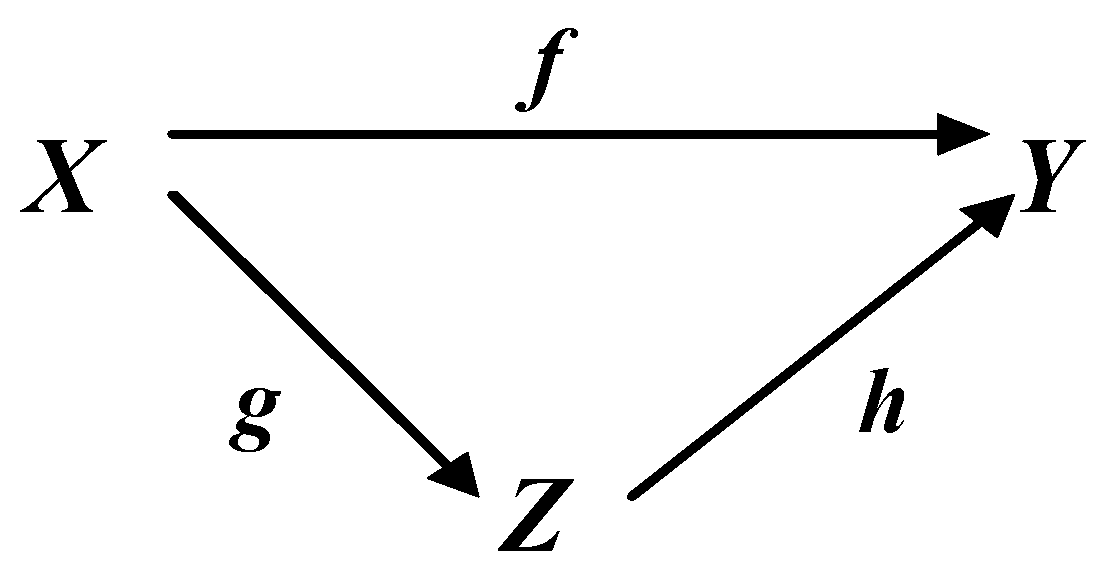
We will consider the commutative diagram shown in Figure 1. Many commutative diagrams are brought to such a diagram in problems of algebraic system theory [3]. The realization theorem (Theorem 1) [1,2,3] is valid for the diagram, the formulation of which is given here for completeness.

Theorem 1.

Realization theorem: If the map f:X→Y is a usual isomorphism and there are maps g:X→Z and h:Z→Y such that the composition f = hg is true, then the maps g and h are isomorphisms up to isomorphism f.

Concerning the composition of hg of maps g and h, we can say that it implements, models the map-isomorphism f. It should be emphasized that the map f must be isomorphic outside the commutative diagram, that is, it must be an ordinary, “unconditional” isomorphism. On maps g and h the theorem states that even if these maps separate, outside the composition and the commutative diagram, they are not isomorphisms, then as part of the composition f = hg, closed by the isomorphism f in the commutative diagram, become isomorphisms up to the isomorphism f, that is, become “relative isomorphisms”—isomorphisms with respect to (up to) the isomorphism f. This means that each of the maps g and h is an isomorphism only and strictly within the commutative map diagram shown in Figure 1. Under these conditions, the maps g and h in the commutative diagram satisfy all the properties of isomorphic maps defined in algebra [28]. The proof is given in [3]. However, there is a need to reproduce here a considerable part of the proof of the implementation theorem from [3] for a more understandable presentation of the rules of definition of the inverse mappings g and h in the commutative diagram. This is done below directly when considering these rules.

The simplest explanation of the realization theorem is as follows. The composition of the mappings g and h forms a system in which these mappings have a new property, the property of having a reverse mapping. This property may not be present in each of them individually, outside of this system. This is a manifestation of emergence—the main sign of the emergence of any new system. Consider, for example, two children. Together they can play hide-and-seek, and each child separately, outside the “children” system, can not hide from himself. The “hide” property is a systemic property of the “children” system, a manifestation of its emergence. At the same time, the bystander can see the hidden child: the property of “hiding” belongs only to the system “children”. So the property of reversibility of maps g and h is manifested only in the system-composition, realizing or commuting some unconditional isomorphism. The realization theorem describes (formalizes) in the most General form the occurring of the emergence effect and in this sense is the most General mathematical definition of the system as a mathematical abstraction and a phenomenon of real reality.

Since the maps g and h in the commutative diagram are isomorphisms, they must have the only inverses g⁻¹ and h⁻¹ in this diagram. We define these inverses for two cases:

1)

In the first case, all maps f, g, and h and the composition f = hg in the commutative diagram in Figure 1 are defined initially. In many problems of system theory there is a need to determine the inverses of g⁻¹ and h⁻¹ explicitly;

2)

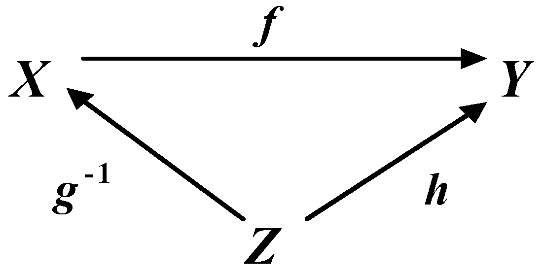
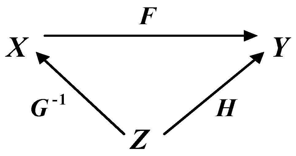
In the second case, the commutative diagram is converted to the form shown in Figure 2. Here, only the isomorphic map f, some map designated as g⁻¹, and their composition fg⁻¹ are initially known. It is clear that under these conditions the map h commuting the specified composition exists, is uniquely and immediately determined by the formula fg⁻¹ = h. In this case, the mapping of h⁻¹ is unknown and needs to be determined. The inverse of g⁻¹, which also needs to be determined, is also unknown. However, maps g and h⁻¹, inverses to g⁻¹ and h, respectively, can be defined only up to class, that is, they are not unique. This is because, based on the requirements of the realization theorem [3], in this case a pair of mappings (h, g) and their composition hg = f, which implement the isomorphism of f, or a pair of mappings (g⁻¹, h⁻¹) and their composition g⁻¹h⁻¹ = f⁻¹, which implement the isomorphism f⁻¹, are not determined initially and at the same time. Thus, in this second case it is required to find classes of admissible maps h⁻¹ and g that satisfy the condition fg⁻¹ = h and other conditions of the realization theorem, which will be given below. It is obvious that the required classes of maps h⁻¹ and g will be strictly interconnected taking into account these conditions. Once you have defined the classes of valid mappings, you can select one related mappings instance from the corresponding classes, if necessary, and commit those instances to the commutative diagram. Only in this case the only inverses to these instances of mappings will be fixed and can be calculated. Clearly, after fixing specific instances of mappings from valid classes, this case is no different from the first case where all mappings in a commutative diagram are known.

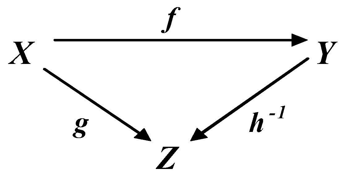
The case shown in Figure 2, is typical, for example, for the application of the realization theorem to the problem of determining regulators in the theory of systems [3,25]. The case of determination of observers—see Figure 3—considered in [3,26] is also equivalent to it. In defining observers, the difference is that the isomorphic map f, some map designated as h⁻¹, and their composition h⁻¹f = g are known and defined in advance. The problem is to define maps h and g⁻¹. By analogy with Figure 2, maps of h and g⁻¹ in Figure 3 can be defined up to class. Due to the equivalence of the problem statements illustrated in Figure 2 and Figure 3, in the future we will solve only the problem reflected in the commutative diagram in Figure 2.

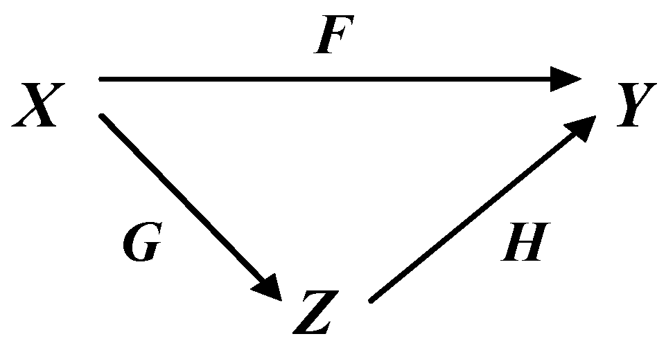
We will start with the first case and Figure 1, when in the commutative diagram the composition f = hg and all maps f, g, and h are initially defined. And f is such that it is an isomorphism outside the commutative diagram. Based on the realization theorem, it is known [3] that in this case the only inverses g⁻¹ and h⁻¹ in the commutative diagram exist. To find them is required. It is clear that the inverses of g⁻¹ and h⁻¹, based on the conditions of the theorem and the equations obtained on its basis, must be completely determined by the original maps f, g, and h. We try to express the inverses of g⁻¹ and h⁻¹ through the original known maps and thus obtain rules for their computation.

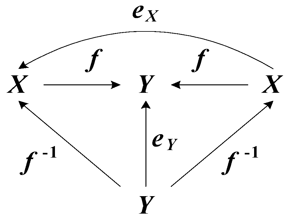
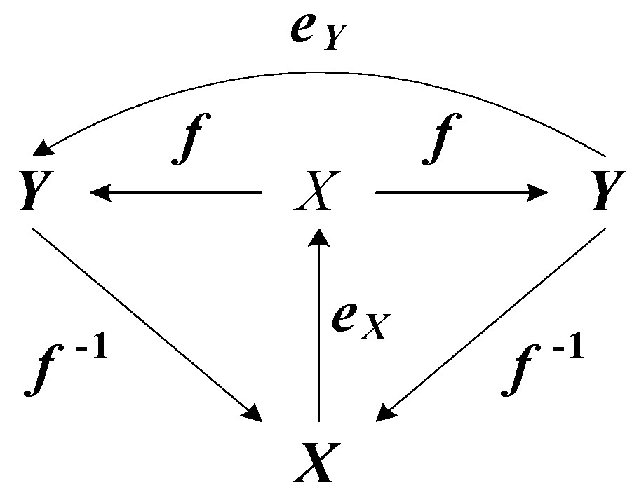
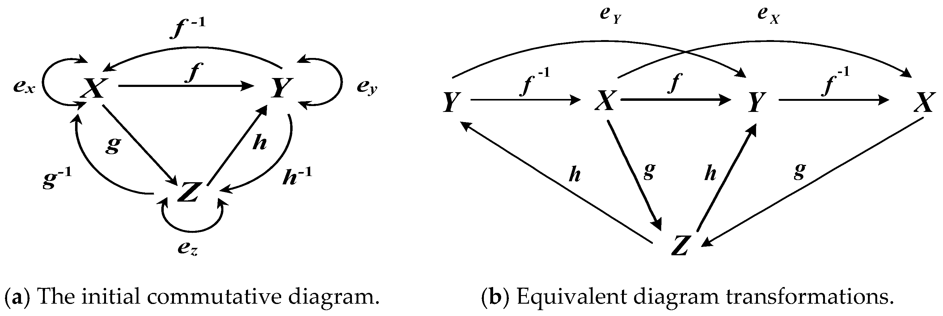
Directly from the commutative diagram shown in Figure 1 (see also the supporting diagrams in Figure 4, Figure 5, Figure 6, Figure 7, Figure 8 and Figure 9, by virtue of isomorphism in the usual sense of the map f, the equalities follow

e_x^right = f⁻¹f, e_y^left = ff⁻¹, e_x^left = g⁻¹g, e_y^right = hh⁻¹, f⁻¹ = e_xf⁻¹, f⁻¹ = f⁻¹e_y,
e_x = e_x^right = e_x^left = e_y^right = e_y^left = e_y = e.

(1)

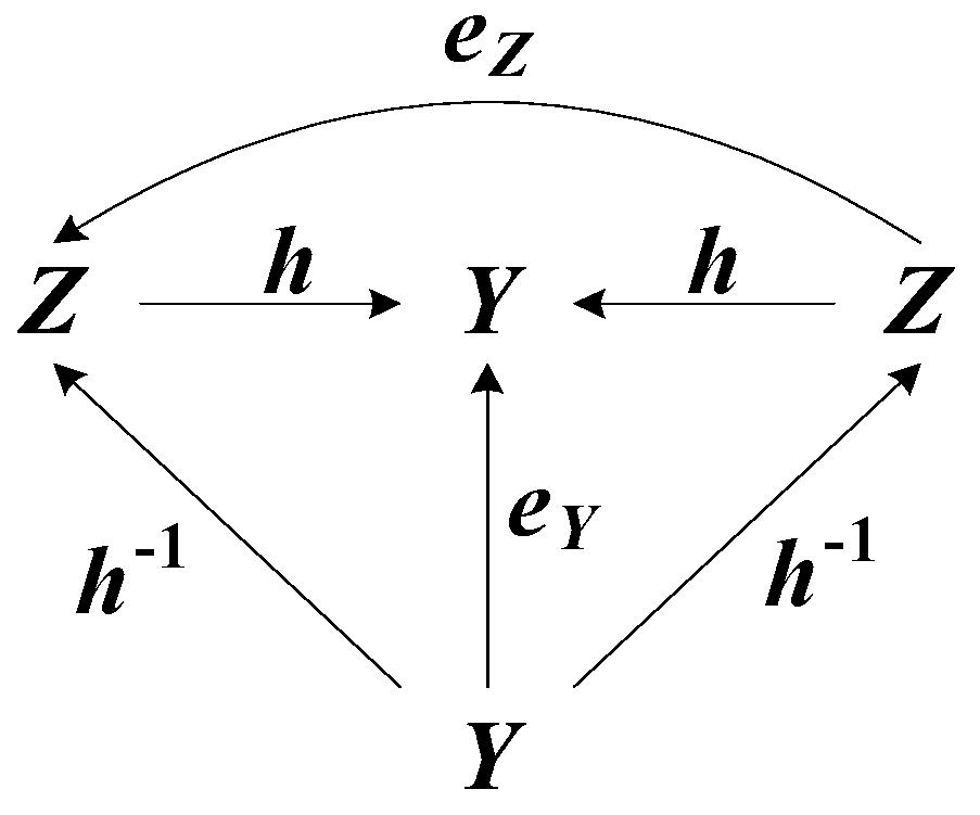
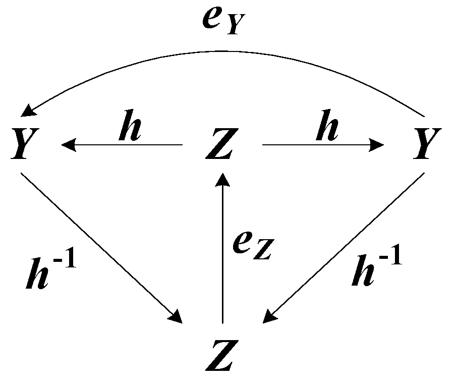
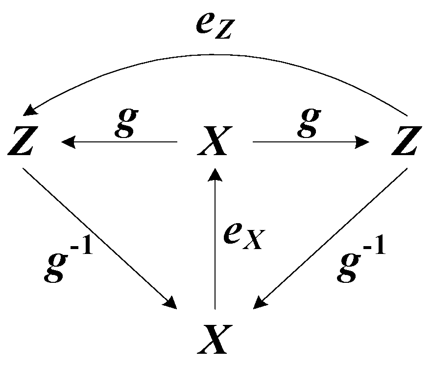
Here e_x^right, e_x^left are the right and left units on X; e_y^right, e_y^left are the right and left units on Y. By virtue of the uniqueness of the map f⁻¹ (since by the condition f is the usual isomorphism), the maps e_x and e_y are also unique and equal to e, where e is the usual unit map such that e = ee = ee⁻¹ = e⁻¹ e= e^-1. From the auxiliary diagrams constructed on the basis of the initial diagram and given in Figure 6, Figure 7, Figure 8 and Figure 9, the equalities follow

h⁻¹ = e_zh⁻¹, h⁻¹ = h⁻¹e_y, g⁻¹ = g⁻¹e_z, g⁻¹ = e_xg⁻¹,

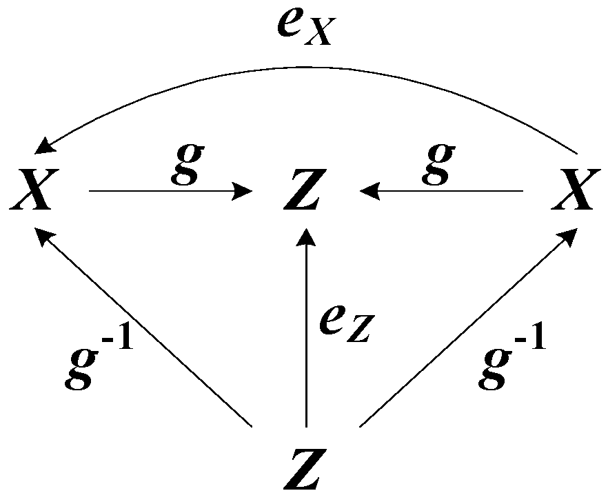
where e_z is some unit on Z. From the auxiliary diagrams shown in Figure 10b, it is also possible to obtain equality

f⁻¹ = g⁻¹h⁻¹, e_z^left = gg⁻¹, e_z^right = h⁻¹h,

where e_z^left, e_z^right are left and right units on Z.

In the proof of the realization theorem in [3] it is shown that in the commutative diagram in Figure 1 and Figure 10a the following equalities are true

e_z^left = gg⁻¹, e_z^right = h⁻¹h, e_z^left = e_z^right = e_z, e_z^lefte_z^right= e_z, e_z^righte_z^left = e_z, (e_z)⁻¹= e_z, e_z e_z= e_z.

(2)

It follows from (2) that

e_z^lefte_z^right = e_z^righte_z^left,

that is

gg⁻¹h⁻¹h = h⁻¹hgg⁻¹.

Then, taking into account equations f⁻¹ = g⁻¹h⁻¹ and f = hg, we obtain

g f⁻¹h = h⁻¹ f g⁻¹.

It is obvious that there exists a composition of map g⁻¹ and each of the parts of this equality. “Multiply” the equation by g⁻¹ on the left side, we get

g⁻¹g f⁻¹h = g⁻¹h⁻¹ f g⁻¹.

(3)

Since g⁻¹h⁻¹ = f⁻¹, the right part of equality (3) gets the form

f⁻¹f g⁻¹ = 〈e_x^right = f ⁻¹f〉 = e_x^rightg⁻¹ = 〈e_x^right = e_x^left = e〉= g⁻¹.

Taking into account e_x^left = g⁻¹g we write the left side of the equality (3) in the form

e_x^leftf⁻¹h = 〈e_x^left f⁻¹ = f⁻¹〉= f⁻¹h = g⁻¹, ⇒ f⁻¹h = g⁻¹.

That is, finally

g⁻¹ = f ⁻¹h.

(4)

Here h is initially known, and f⁻¹ can be easily computed, since f is also a known ordinary isomorphic map for which the inverse of f⁻¹ is known to exist. Similarly, it can be shown that

h⁻¹ = g f⁻¹.

(5)

The equality (5) can also be directly verified by the commutative diagram shown in Figure 10а. Here also all the mappings are known on the right side.

Thus, the inverses of g⁻¹ and h⁻¹ can be quite simply calculated from the known map included in the original commutative diagram. Making sure that the g⁻¹ and h⁻¹ mappings are indeed inverses to the corresponding original mappings in the commutative diagram shown in Figure 1, it is possible by their direct substitution in equality (2), the validity of which must be ensured in accordance with the conditions of the realization theorem [3]. Indeed

e_z^left = g g⁻¹ = 〈g⁻¹ = f⁻¹h〉 = g f⁻¹h and e_z^right = h⁻¹h = 〈h⁻¹ = g f⁻¹〉 = g f⁻¹h ⇒ e_z^left = e_z^right = e_z.
e_z^lefte_z^right = gf⁻¹hgf⁻¹h = 〈hg = f〉 = gf⁻¹f f⁻¹h = 〈f⁻¹f = e_x^right, ff⁻¹ = e_y^left〉 = gf⁻¹e_y^lefth =
= g e_x^right f⁻¹h = 〈f⁻¹e_y^left = f⁻¹, e_x^right f⁻¹ = f⁻¹〉 = g f⁻¹h = e_z.

Thus, Equations (4) and (5) for calculating the inverses of g⁻¹ and h⁻¹ are true and can be applied inside the commutative diagram shown in Figure 1. For example, in the simple case where the original isomorphism f—is the usual unit map (in the case of matrices—the usual unit matrix), that is

f = f⁻¹ = e,

the inverses g⁻¹ and h⁻¹ are trivial and do not require computation, since in this case g⁻¹ = h and h⁻¹ = g are always true. This can be seen from the auxiliary diagram in Figure 10b, from which it follows that eh = h and ge = g.

At first glance, Equations (4) and (5) could be written directly from the commutative diagrams shown in Figure 1 and Figure 10a. In fact, these equations are not as trivial as they may seem, because the inverses of maps g and h outside the commutative diagram may not exist. These arguments just allowed us to prove the existence of inverses g⁻¹ and h⁻¹ in the commutative diagram, partly repeating the proof of the realization theorem [3], and strictly derive Equations (4) and (5) for their calculation.

Consider the examples of calculating the inverses for the first case when matrices are used as mappings in the original diagram in Figure 1. The commutative diagram for matrices is shown in Figure 11.

Example 1.

Let the matrices have the following structure:

$$F=\left[\begin{array}{cc}1& 0\\ 0& 1\end{array}\right],G=\left[\begin{array}{cc}1& -1\\ 0& 1\\ 1& 1\end{array}\right],H=\left[\begin{array}{ccc}0.5& 0& 0.5\\ 0& 1& 0\end{array}\right],X=\left[\begin{array}{c}{x}_1\\ x_2\end{array}\right],Y=\left[\begin{array}{c}{y}_1\\ y_2\end{array}\right].$$

(6)

It is clear that F isomorphism and composition F = HG are true, which corresponds to the conditions of the realization theorem. Hence, as follows from this theorem, despite the fact that matrices H and G are rectangular and in the usual sense irreversible, inside the commutative diagram they must have the only inverses up to isomorphism F. Since F is a usual unit matrix, then according to (4) and (5) in this case G⁻¹ = H and H⁻¹ = G, that is,

$$G^{-1}=\left[\begin{array}{ccc}0.5& 0& 0.5\\ 0& 1& 0\end{array}\right],H^{-1}=\left[\begin{array}{cc}1& -1\\ 0& 1\\ 1& 1\end{array}\right].$$

(7)

You can verify that matrices G⁻¹ and H⁻¹ in (7) are indeed the only inverses to matrices G and H in the commutative diagram, since they satisfy all conditions of (1) and (2).

Example 2.

Here the matrices have the following structure [3]:

$$F=\left[\begin{array}{cc}1& 0\\ b{a}^{-1}& 0\end{array}\right],G=\left[\begin{array}{cc}1& 0\end{array}\right],H=\left[\begin{array}{c}1\\ b{a}^{-1}\end{array}\right],X=\left[\begin{array}{c}a\\ b\end{array}\right],Y=\left[\begin{array}{c}a\\ b\end{array}\right].$$

(8)

Composition $F=HG$ is also valid. In [3] it is shown that the realization theorem is also valid in the wider case—for isomorphisms that are such not only in the usual sense—outside the commutative diagram—but also have special properties. So, in this case, isomorphism F has the peculiarity that its structure depends on the structure of mapping matrices X, Y. Indeed, it is quite obvious that the determinant of matrix F is zero and it has no inverse in the usual sense. At the same time, we can make sure that for matrix F, the structure of which is determined by the rules (8), there is an inverse (in the algebraic sense [28]) matrix

$$F^{-1}=F{F}^{-1}=F^{-1}F=FF=F^{-1}{F}^{-1}=F=\left[\begin{array}{cc}1& 0\\ b{a}^{-1}& 0\end{array}\right].$$

That is, F is isomorphism. From relations (4), (5) it is possible to find inverse matrices:

$$G^{-1}=\left[\begin{array}{c}1\\ b{a}^{-1}\end{array}\right],H^{-1}=\left[\begin{array}{cc}1& 0\end{array}\right].$$

All conditions (1) and (2) necessary to satisfy the realization theorem are satisfied.

Consider the second case with respect to the commutative diagram shown in Figure 12. Here, only the isomorphic map F is known, as well as some map designated as G⁻¹, and their composition FG⁻¹ = H. Moreover, H is unique, since maps F and G⁻¹ are completely (up to an instance) determined. However, maps G and H⁻¹ to be defined, which are inverse to G⁻¹ and H, respectively, are not unique in this case and can only be defined up to class precision. This, as mentioned above, follows from the realization theorem [3]: In this case, a pair of maps (H, G) and their composition HG = F, which implements the isomorphism F, or a pair of maps (G⁻¹, H⁻¹) and their composition G⁻¹H⁻¹ = F⁻¹, which implements the isomorphism F⁻¹, are not defined initially and simultaneously.

In this second case it is required to find classes of interconnected mappings H⁻¹ and G admissible under the condition FG⁻¹ = H and conditions in form (1), (2). After definition of classes, proceeding from additional considerations, it is possible to choose one instance of mappings per class and to fix these instances in the commutative diagram. For fixed instances of mappings, the only inverses can be calculated. After fixing specific instances of mappings from a valid class, this case is no different from the first case where all mappings in a commutative diagram are known initially.

Thus, the task of the second case is to determine the classes of admissible maps H⁻¹ and G by known conditions in the form (1), (2), and the condition FG⁻¹ = H. These conditions are sufficient to determine the classes of maps H⁻¹ and G, and, if necessary, their specific instances. Let us demonstrate this with an example.

Example 3.

Let the matrices have the following structure on Figure 12:

$$F=\left[\begin{array}{cc}1& 0\\ 0& 1\end{array}\right],G^{-1}=\left[\begin{array}{ccc}0.5& 0& 0.5\\ 0& 1& 0\end{array}\right],X=\left[\begin{array}{c}{x}_1\\ x_2\end{array}\right],Y=\left[\begin{array}{c}{y}_1\\ y_2\end{array}\right].$$

(9)

Then $H=\left[\begin{array}{ccc}0.5& 0& 0.5\\ 0& 1& 0\end{array}\right]$ can be immediately determined out of the condition FG⁻¹ = H. The size and structure of matrices H⁻¹ and G are determined, taking into account the size of matrices G⁻¹ and H in (9) from equality

$$G=H^{-1}=G{F}^{-1}=\left[\begin{array}{cc}{k}_1& k_2\\ k_3& k_4\\ k_5& k_6\end{array}\right],$$

(10)

where unknown elements k₁ … k₆ must be calculated from conditions in the form (1), (2). Given the fact that F is an ordinary identity matrix, FG⁻¹ = H, H⁻¹F = G ⇒ G⁻¹ = H and H⁻¹ = G, we can write

$$e_z^{left}=G{G}^{-1}=e_z^{right}=H^{-1}H=\left[\begin{array}{ccc}0.5k_1& k_2& 0.5k_1\\ 0.5k_3& k_4& 0.5k_3\\ 0.5k_5& k_6& 0.5k_6\end{array}\right]=e_z,$$

(11)

$$e_x^{left}=G^{-1}G=e_y^{right}=H{H}^{-1}=\left[\begin{array}{cc}\left(0.5k_1+0.5k_5\right)& \left(0.5k_2+0.5k_6\right)\\ k_3& k_4\end{array}\right]=e=\left[\begin{array}{cc}1& 0\\ 0& 1\end{array}\right].$$

(12)

From (12) we obtain equality

0.5k₁ + 0.5k₅ = 1; 0.5k₂ + 0.5k₆ = 0; k₃ = 0; k₄ = 1.

(13)

Thus, the problem of calculating matrices H⁻⁻¹ = G up to a class in the form (10) is solved. The relationships of the matrix elements in (10) are determined by Equations (12) and (13), in which there is freedom of choice for the two elements. Equality (11) can be used to check the feasibility of conditions in the form (2). Set k₁ = 2, k₂ = 1. Then, from (13) we get k₅ = 0, k₆ = −1, and a specific instance of the matrix will be in the form

$$G=H^{-1}=\left[\begin{array}{cc}2& 1\\ 0& 1\\ 0& -1\end{array}\right].$$

(14)

Checking of matrices (10) and (14) according to the formulas in the form (1) and (2) shows their full compliance with all the conditions applicable in the commutative diagrams in Figure 11 and Figure 12. You may verify that the following matrices are the only inverses for fixed instances of matrices (14) in the commutative diagram in Figure 11.

$$G^{-1}=H=\left[\begin{array}{ccc}0.5& 0& 0.5\\ 0& 1& 0\end{array}\right].$$

(15)

In this example, matrix G⁻¹ in (9) was specifically chosen to be equal to matrix G⁻¹ in (7) from the first example. It is easy to verify that matrices H⁻¹ = G from the first example belong to class (10). Indeed, if we set (13) k₁ = 1, k₂ = −1, we get k₅ = 1, k₆ = 1. Then from (10) and (13) we get other instances of matrices of class (10)

$$H^{-1}=G=\left[\begin{array}{cc}1& -1\\ 0& 1\\ 1& 1\end{array}\right].$$

(16)

Comparison of matrices (16) with the corresponding matrices from (6) and (7) of example 1 shows their coincidence. For fixed instances (16) of matrices H⁻¹ = G in commutative diagrams in Figure 11 and Figure 12 there are the only inverses H = G⁻¹ defined by relations (6) and (7) from the first example.

Examples 1 and 3 are interesting in the way that they demonstrate not only the rules for determining inverses in commutative diagrams satisfying the conditions of the realization theorem [3], but also illustrate the principle of relativity in mathematics formulated in [3]: The same map can have different inverses up to the same isomorphism in different compositions with other maps commuting this isomorphism. Moreover, these inverses are the only ones in their compositions realizing (commuting) the same isomorphism. So, in example 1 a pair of mappings in (6)

$$G=\left[\begin{array}{cc}1& -1\\ 0& 1\\ 1& 1\end{array}\right],H=\left[\begin{array}{ccc}0.5& 0& 0.5\\ 0& 1& 0\end{array}\right],$$

(17)

commuting isomorphism $F=\left[\begin{array}{cc}1& 0\\ 0& 1\end{array}\right]$ in the diagram in Figure 11, has inverses (7)

$$G^{-1}=\left[\begin{array}{ccc}0.5& 0& 0.5\\ 0& 1& 0\end{array}\right],H^{-1}=\left[\begin{array}{cc}1& -1\\ 0& 1\\ 1& 1\end{array}\right].$$

(18)

In Example 3, a pair of mappings (14) and (15)

$$G=\left[\begin{array}{cc}2& 1\\ 0& 1\\ 0& -1\end{array}\right],H=\left[\begin{array}{ccc}0.5& 0& 0.5\\ 0& 1& 0\end{array}\right],$$

(19)

commuting the same isomorphism $F=\left[\begin{array}{cc}1& 0\\ 0& 1\end{array}\right]$, has inverses

$$G^{-1}=\left[\begin{array}{ccc}0.5& 0& 0.5\\ 0& 1& 0\end{array}\right],H^{-1}=\left[\begin{array}{cc}2& 1\\ 0& 1\\ 0& -1\end{array}\right].$$

(20)

3. Discussion

Thus, the same map H in different compositions (17) and (19) commuting the same isomorphism F has different inverses (18) and (20) and these inverses are the only ones in their compositions. The algebraic principle of relativity in relation to the theory of systems is interpreted in [3] as follows: the same element (characterized by some mapping) in combination with different elements in different systems can exhibit different properties and even properties that it did not have outside the system at all—for example, the property of having an inverse map to the map being its model. This allowed us to assert [3] that the theorem of realization and the corresponding mathematical (algebraic) principle of relativity strictly formally reveal and explain the mechanism of occurrence of the emergent property in systems (including physical ones). Emergence as a phenomenon and property is the main feature of the system and a key element of the meaningful definition of “system” [3,29,30,31,32,33]. This property appears due to “system effect”: In the system, created as a result of combining some elements in it, new properties arise and manifest themselves, which are not reduced to the sum of the properties of the elements united in the system, as well as the elements in the system manifest new properties they lack outside the system.

4. Summary

In the article, based on the conditions arising from the realization theorem [3], formal rules for determining the inverses of maps forming a composition, commuting (implementing) some isomorphism are obtained. The rules are obtained for commutative diagrams corresponding to different cases of setting initial maps and their compositions commuting a known ordinary isomorphism.

References

- Kulabukhov, V.S. Printsip izomorfnosti v teorii sistem. In Proceedings of the Mezhdunarodnaya Konferentsiya po Problemam Upravleniya, IPU RAN, Moscow, Russia, 29 June–2 July 1999; Volume 1. [Google Scholar]
- Kulabukhov, V.S. Printsip izomorfnosti v zadache realizatsii i yego prilozheniya k analizu svoystv sistem upravleniya. In Proceedings of the XII Vserossiysk, Soveshch, po Problemam Upravleniya VSPU-2014, IPU RAN, Moscow, Russia, 16–19 June 2014; pp. 438–448. [Google Scholar]
- Kulabukhov, V.S. The General Principle of Isomorphism in Systems Theory. Available online: https://cloudofscience.ru/sites/default/files/pdf/CoS_5_400.pdf (accessed on 7 May 2019).
- Kalman, R.E. On the General Theory of Control System. IFAC Proc. Vol. 1960, 1, 18–22. [Google Scholar] [CrossRef]
- Wang, P. Invariance, uncontrollability, and unobservaility in dynamical systems. IEEE Trans. Autom. Control 1965, 10, 366–367. [Google Scholar] [CrossRef]
- Luenberger, D. Observers for multivariable systems. IEEE Trans. Autom. Control 1966, 11, 190–197. [Google Scholar] [CrossRef]
- Zade, L.; Desoer, C.A.; Zadeh, L.A. Teoriia Lineinykh System; Nauka: Moscow, Russia, 1970. [Google Scholar]
- Kalman, R.E.; Arbib, M.A.; Falb, P.L. Ocherki po Matematicheskoi Teorii Sistem; Mir: Moscow, Russia, 1971. [Google Scholar]
- Mesarovic, M.D. Conceptual basis for a mathematical theory of general systems. Kybernetes 1972, 1, 35–40. [Google Scholar] [CrossRef]
- Takahara, Y. Realization Theory for General Stationary Linear Systems and General System Theoretical Characterization of Linear Differential Equation Systems. Trans. Soc. Instrum. Control Eng. 1973, 9, 408–414. [Google Scholar] [CrossRef] [Green Version]
- Mesarovic, M.; Takahara, Y. General Systems Theory: Mathematical Foundations (Mathematics in Science and Engineering); Elsevier: Amsterdam, The Netherlands, 1975. [Google Scholar]
- Sain, M.K. The growing algebraic presence in systems engineering: An introduction. Proc. IEEE 1976, 64, 96–111. [Google Scholar] [CrossRef]
- Agazzi, E. Systems theory and the problem of reductionism. Erkenntnis 1978, 12, 339–358. [Google Scholar] [CrossRef]
- Willems, J.C. In Dynamical Systems and Microphysics. In System Theoretic Foundations for Modelling Physical Systems; Springer: Vienna, Austria, 1980; pp. 279–289. [Google Scholar]
- Li, T. On the realization theory of impulse response sequences. Acta Math. Sci. 1984, 4, 365–376. [Google Scholar] [CrossRef]
- Kalman, P.E. Identifikatsiya sistem s shumami. Uspekhi Mat. Nauk Russ. 1985, 40, 27–41. [Google Scholar]
- Krasovskii, A.A. Handbook on the Theory of Automatic Control; Nauka: Moscow, Russia, 1987. [Google Scholar]
- Proychev, T.P.; Mishkov, R.L. Transformation of nonlinear systems in observer canonical form with reduced dependency on derivatives of the input. Automatica 1993, 29, 495–498. [Google Scholar] [CrossRef]
- Ciccarella, G.; Dalla Mora, M.; Germani, A. A Luenberger-like observer for nonlinear systems. Int. J. Control 1993, 57, 537–556. [Google Scholar] [CrossRef]
- Bukov, V.N.; Kulabukhov, V.S.; Maksimenko, I.M.; Ryabchenko, V.N. Uniqueness of solutions of problems of the theory of systems. Autom. Remote Control 1997, 58, 1875–1885. [Google Scholar]
- Bukov, V.; Kulabuhov, V.; Maximenko, I.; Ryabchenko, V. Uniqueness of a solution of the systems theory problems and functional integration. In Proceedings of the IFAC Conference on Informatics and Control, St. Petersburg, Russia, 9–13 June 1997; Volume 2. [Google Scholar]
- Bukov, V.N. Vlozheniye Sistem. Analiticheskiy Podkhod k Analizu i Sintezu Matrichnykh System; Izd-vo nauchn. Literatury N.F. Bochkarevoy: Kaluga, Russia, 2006. [Google Scholar]
- Bhattacharyya, S.P.; Datta, A.; Keel, L.H. Linear Control Theory: Structure, Robustness and Optimization; CRC Press: Boca Raton, FL, USA, 2009. [Google Scholar]
- Isidori, A. Nonlinear Control Systems; Springer Science & Business Media: Berlin, Germany, 2013. [Google Scholar]
- Kulabukhov, V. Linear Isomorphic Regulators. In MATEC Web of Conferences, Proceedings of the CMTAI2016, Moscow, Russsia, 15–16 December 2016; MATEC Web of Conferences: Paris, France, 2017; Volume 9, p. 03008. [Google Scholar] [CrossRef]
- Kulabukhov, V.S. Isomorphic observers of the linear systems state. In IOP Conference Seriesm, Proceedings of the Materials Science and Engineering in Aeronautics (MEA2017), Moscow, Russian Federation, 15–16 November 2017; IOP Publishing: Bristol, UK, 2017; Volume 312, p. 012016. [Google Scholar] [CrossRef]
- Kulabukhov, V. Algebraic Formalization of System Design Based on a Purposeful Approach. In IOP Conference Series: Materials Science and Engineering; IOP Publishing: Bristol, UK, 2019; Volume 476, p. 012017. [Google Scholar] [CrossRef]
- Kostrikin, A.I. Vvedenie v Algebru: Osnovy Algebry; Fiziko-Matematicheskaia Literatura: Moscow, Russia, 1994. [Google Scholar]
- Homyakov, D.M.; Homyakov, P.M. Fundamentals of System Analysis; Lomonosov Moscow State University: Moscow, Russia, 1996. [Google Scholar]
- Zhilin, D.M. Teoriya Sistem: Opyt Postroyeniya Kursa; KomKniga: Moscow, Russia, 2006. [Google Scholar]
- Volkova, V.N.; Denisov, A.A. Osnovy Teorii Sistem i Sistemnogo Analiza; Izdatel’stvo SPbGTU: Saint-Petesburg, Russia, 1999. [Google Scholar]
- Artyukhov, V.V. Obshchaya Teoriya Sistem: Samoorganizatsiya, Ustoychivost’, Raznoobraziye, Krizisy; Knizhnyy dom LIBROKOM: Moscow, Russia, 2010. [Google Scholar]
- Urmantsev, Y.A. Obshchaya teoriya sistem: Sostoyaniye, prilozheniya i perespektivy razvitiya. In Sistema, Simmetriya, Garmoniya; Mysl’: Moscow, Russia, 1988. [Google Scholar]
Figure 1.
Commutative diagram to the realization theorem.
Figure 2.
Commutative diagram for the 2nd case.
Figure 3.
Equivalent commutative diagram for the 2nd case.
Figure 4.
Auxiliary diagram 1.
Figure 5.
Auxiliary diagram 2.
Figure 6.
Auxiliary diagram 3.
Figure 7.
Auxiliary diagram 4.
Figure 8.
Auxiliary diagram 5.
Figure 9.
Auxiliary diagram 6.
Figure 10.
Auxiliary commutative diagrams.
Figure 11.
Commutative diagram for matrices.
Figure 12.
Commutative diagram for the second case.
© 2019 by the author. Licensee MDPI, Basel, Switzerland. This article is an open access article distributed under the terms and conditions of the Creative Commons Attribution (CC BY) license (http://creativecommons.org/licenses/by/4.0/).
Share and Cite
MDPI and ACS Style
Kulabukhov, V.S. A General Principle of Isomorphism: Determining Inverses. Symmetry 2019, 11, 1301. https://doi.org/10.3390/sym11101301
AMA Style
Kulabukhov VS. A General Principle of Isomorphism: Determining Inverses. Symmetry. 2019; 11(10):1301. https://doi.org/10.3390/sym11101301
Chicago/Turabian StyleKulabukhov, Vladimir S. 2019. "A General Principle of Isomorphism: Determining Inverses" Symmetry 11, no. 10: 1301. https://doi.org/10.3390/sym11101301
Note that from the first issue of 2016, this journal uses article numbers instead of page numbers. See further details here.