A Symmetry-Breaking Node Equivalence for Pruning the Search Space in Backtracking Algorithms

Abstract

We introduce a new equivalence on graphs, defined by its symmetry-breaking capability. We first present a framework for various backtracking search algorithms, in which the equivalence is used to prune the search tree. Subsequently, we define the equivalence and an optimization problem with the goal of finding an equivalence partition with the highest pruning potential. We also position the optimization problem into the computational-complexity hierarchy. In particular, we show that the verifier lies between $\mathcal{P}$ and $\mathcal{NP}$-complete problems. Striving for a practical usability of the approach, we devise a heuristic method for general graphs and optimal algorithms for trees and cycles.

1. Introduction

The work presented in this paper was primarily motivated by the subgraph isomorphism problem, the goal of which is to find a single (or all, depending on the definition) occurrence(s) of a given pattern graph G in a given host graph H. This problem has numerous applications in fields such as chemistry, where it is often of interest to search for a specific substructure (e.g., a functional group) within a larger structure (e.g., a molecule) [1]. Subgraph isomorphism is also a key component of graph grammar parsing [2,3]; to determine whether a given graph G can be generated by a given graph grammar, the graphs on the productions’ right-hand sides have to be matched against subgraphs of the graph G.

The decision version of the subgraph isomorphism problem is $\mathcal{NP}$-complete [4], and its counting version is $\#\mathcal{P}$-complete [5]. A polynomial-time algorithm is therefore unlikely to exist. Besides that, none of the algorithms developed thus far perform in the worst case any better than a naive occurrence enumeration approach [6]. Most of the exact algorithms are based on backtracking (e.g., [7,8,9,10,11,12]), utilizing different pruning techniques to reduce the search space. However, when designing a practically efficient backtracking algorithm, pruning is not the only parameter that influences its speed. A very important factor is the overhead that is required for these techniques to work (such as bookkeeping and computations that have to be done at every node of the search tree). Symmetry-breaking is one possible technique that reduces the search space significantly, but has not been utilized in any subgraph-isomorphism solver. The biggest reasons for this are the complexity of implementation and a large overhead which ultimately leads to slower algorithms.

To address this problem, we introduce a novel approach to symmetry-breaking whose main goal is to be lightweight and suitable for implementation in state-of-the-art solvers and not so much to encompass as much symmetries as possible. Our approach is based on a type of equivalence on graph vertices, called exploratory equivalence (EE). Exploratory equivalence induces an exploratory equivalent partition of the vertex set. As shown below, if a set of vertices (say, P) is an equivalence class in an EE partition of the pattern graph G, then the vertices in P can be regarded as being interchangeable during the search for occurrences of G in the host graph H, reducing the number of distinguishable mappings between the vertices in P and those of the graph H by a factor of $\left|P\right|!$.

Since several EE partitions can be defined for a pattern graph with more than one automorphism, a problem that immediately arises is that of finding an EE partition that brings about the greatest speedup in the subgraph isomorphism search. We define this problem as the maximum EE partition problem (MaxEE).

Although the subgraph isomorphism problem was our initial motivation, the concept has a much broader application. As we demonstrate, exploratory equivalence can be used to speed up backtracking algorithms for a wide variety of search problems.

The main contributions of this paper are the following:

• The definition of a novel vertex equivalence on graphs, which is simple to use in various backtracking algorithms and, even more importantly, very lightweight, i.e., it introduces very little computational overhead on the existing backtracking algorithms.
• Even though we start with the subgraph isomorphism, we show that exploratory equivalence can be applied to a broader set of search problems. Whenever the goal of the problem in question is to find an injective mapping between a given pair of sets that satisfies a certain predicate, exploratory equivalence can be used to speed up the backtracking-based search approach. Furthermore, the EE-based performance improvement technique that we describe in this paper can be employed in addition to other search-space pruning methods, not just instead of them.
• We analyze the computational complexity of the defined optimization problem. More precisely, we show that the verifier for the optimization problem is at least as hard as the graph isomorphism problem and at most as hard as the setwise stabilizer problem. As a consequence, the decision version of MaxEE at present cannot be classified as a member of $\mathcal{NP}$.
• We develop a heuristic method for solving the MaxEE problem. We were able to see the practicality of this method in our practical assessment on a set of realistic graphs.
• For two families of graphs, namely trees and cycles, we provide exact and efficient methods for finding the optimal exploratory efficient partition. For the trees we devise a quadratic algorithm and for cycles we provide an analytic solution that gives a formula for the optimal solution for any cycle.

The rest of this paper is structured as follows. We first discuss the related work in Section 2. In Section 3, we define the concepts and notation that is used throughout the paper. Section 4 generalizes the search problem as a monomorphism search problem and provides a framework in which our equivalence will work. In Section 5, we define exploratory equivalence and the MaxEE problem. Section 6 defines the problem of checking whether a given vertex set partition is exploratory equivalent and determines the lower and the upper bound for its computational complexity. In Section 7, we present two algorithms for solving MaxEE: a suboptimal heuristic algorithm for general graphs and an exact algorithm for trees. In addition, we present an analytic solution for MaxEE on cycle graphs. In Section 8, we apply MaxEE to subgraph isomorphism search and show experimental results on real-world host graphs. Section 9 discusses the proposed approach and concludes the paper.

2. Related Work

Symmetries and symmetry breaking methods have been studied extensively in several contexts, most notably in graph theory, constraint satisfaction problems (CSP), and integer programming (IP). Graph theory has been interested mostly in identifying and describing different types of symmetries, whereas a great deal of work in CSP and IP has delved more into algorithmic aspects of symmetries, i.e., using them to speed up the solvers for these mathematical programs. Our work touches both the way to capture these symmetries and methods to use the presented concepts for speeding up computations. In this section, we summarize the most important related concepts and highlight the similarities and differences with our work.

Graph theory. The basic problem when dealing with symmetries is the graph isomorphism (or more precisely graph automorphism) problem, which is the cornerstone of theoretical computer science. Even though it is still not known to be in $\mathcal{P}$, highly efficient implementations [13] made this problem practical quite some time ago. Even more encouragingly, recent advances by Babai [14] brought this problem much closer to $\mathcal{P}$ also in theory. The practicality of the graph isomorphism problem is highly important in this context, since we heavily rely on existing solvers to produce graph automorphisms and we strive for immediate practical use of the algorithms presented in this paper as well.

In graph theory, the concepts closest to our work are the notions of distinguishing number and distinguishing coloring, defined in [15]. In a nutshell, the distinguishing coloring of a graph is the coloring where the only color-preserving automorphism is the identity. The distinguishing number of a graph is the smallest number of colors for such a coloring. 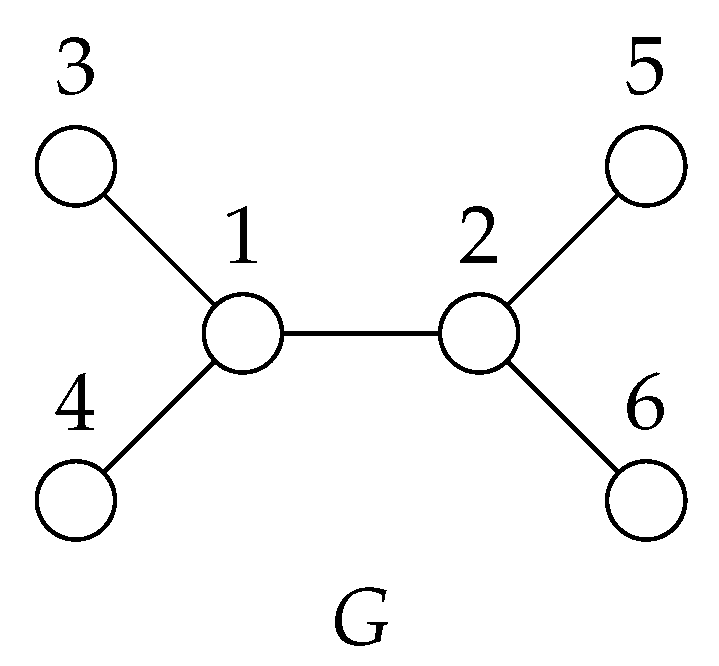Since its definition, it has spawned a large body of work [16,17,18,19], mainly elaborating various families of graphs and dealing with the computational complexity of finding this number. In this paper, we also describe a coloring, but our goal differs in several points. We define a weaker mechanism for symmetry breaking, i.e., we do not strive to capture all symmetries. Instead, our main focus is to define a mechanism that is more amenable to algorithmic usage. By contrast, distinguishing coloring is not directly usable in such applications. Let us give a small example to demonstrate the difference between these two notions. As is clear from the definition in Section 5, the partition $\{1,4,5\mid 2,3,6\}$ is a distinguishing coloring for the graph G in Figure 1, but it is not an exploratory equivalent partition.

Besides distinguishing coloring, graph theory abounds in various other graph equivalences. A graph equivalence is simply a partition (coloration) of the vertex set of a given graph. Although several related notions appear in the literature [20,21,22], exploratory equivalence is, to the best of our knowledge, a novel concept. Everett and Borgatti [20] surveyed a large class of so-called regular partitions. In what follows, we demonstrate that exploratory equivalence does not belong to this class.

Given a partition P, let $C_P\left(v\right)$ denote the class to which the vertex v belongs. Similarly, for a vertex set $S\subseteq V$, let $C_P\left(S\right)$ denote the set of classes assigned to the vertices of S, i.e., $C_P\left(S\right)=\{C_P\left(v\right)\mid v\in S\}$. A partition P of a graph is regular if the equality of the classes of two vertices implies the equality of the classes of the corresponding neighborhoods. More formally, a partition P of a graph G is regular if and only if for all $i,j\in V$ we have

$$C_P\left(i\right)=C_P\left(j\right)\Rightarrow C_P\left(\mathcal{N}\left(i\right)\right)=C_P\left(\mathcal{N}\left(j\right)\right).$$

(1)

Many different types of partitions (i.e., colorations) are regular, e.g., strong and weak structural coloration, orbit coloration, perfect coloration, and exact coloration (see [20] for details). For example, the orbit coloration (i.e., the partition consisting of the orbits) of the graph G in Figure 1 is $\mathcal{P}=\{1,2\mid 3,4,5,6\}$. Incidentally, note this partition is not exploratory equivalent.

As it turns out, exploratory equivalence is not regular. To demonstrate this, consider again the graph G in Figure 1 and its exploratory equivalent partition $\{1,2\mid 3,4\mid 5,6\}$ (again, see Section 5 for definition), with different colors assigned to individual equivalence classes. It is easy to see that this partition is not regular, since $C\left(1\right)=C\left(2\right)$ but $C\left(\right\{3,4\left\}\right)$ is not equal to $C\left(\right\{6,7\left\}\right)$.

CSP, IP, and SAT Symmetry-breaking is a common technique in constraint satisfaction problems, integer programming, and satisfiability [23,24]. Similar to the distinguishing coloring for graphs, Crawford et al. [25] tried to capture all symmetries in any propositional satisfiability problem and demonstrated how it can be used in constraint satisfaction problem. The symmetries are described as a tree of symmetry-breaking predicates that can be used as a preprocessing step for speeding up of search algorithms. However, there are many drawbacks to this approach, most notably: (1) the intractability of producing such a tree; and (2) the potentially exponential size of the resulting tree. Again, our goals are different; we do not wish to capture all the symmetries, but instead strive for the simplicity of the devised mechanism. In addition, we always work with the compact representation of the symmetries, i.e., the polynomial-size generating set of the automorphism group. The resulting exploratory equivalence produces extremely simple symmetry breaking predicates, thus inducing almost no overhead during the search process.

Besides this very general approach, there is an abundance of practical methods in both the area of constraint satisfaction problems, integer programming, and satisfiability (see, e.g., [26,27] for an extensive overview of different methods).

Similar to our idea, the main mechanism for breaking symmetries in CSPs, IPs, and SATs is to apply symmetry breaking constraints, while guaranteeing that no solution (up to automorphisms) is being left out. The methods can roughly be divided into two groups: dynamic symmetry breaking and static symmetry breaking methods. This distinction depends on when the symmetry breaking predicates are computed and enforced. Dynamic methods generate constraints during the search process and have been devised mainly for CSP problems [28]. These methods have also been successfully applied in practice, most notably in the GAP algebra system [29], where it is called Symmetry Breaking During Search (SBDS) [30]. Our method is not dynamic, in the sense that no recomputations of the symmetries are required during the backtracking search.

In contrast to dynamic methods, static methods add inequalities to the initial formulation of the problem. As a special case, the ones most similar to our work and also most widely applied are the methods that add constraints that guide the search algorithm only to a lexicographically smallest solution. There are three major algorithms that work in this manner: Symmetry Backtracking Search (SBS) [31], Symmetry Breaking via Dominance Detection (SBDD) [32,33], and Isomorphism Pruning (IsoP) [34]. These three algorithms were developed independently, but follow the same basic concepts. All of them prune a branch of the enumeration tree if it leads to a lexicographically larger solution. This is enforced by checking whether a certain permutation exists inside the automorphism group. The automorphism group can be kept in a compact representation (i.e., as a set of generators), but checking whether a certain permutation is contained in the group induces a significant overhead at each node of the search tree. Judging from the positive practical results, the costs of group membership checks pay off, but we show below that similar constraints can be enforced without the significant overhead.

3. Preliminaries

Let ${f|}_A$ denote the restriction of a function f to a set A, i.e., the function f defined on $A\cap \mathrm{dom}f$. Let $G=(V,E)$ denote a simple undirected graph, where $V=\{1,2,\cdots ,n\}$ is a set of vertices and $E\subseteq V\times V$ is a set of edges. A connected acyclic undirected graph is called a tree. The set of vertices adjacent to a vertex u is called the neighborhood of u and is denoted $\mathcal{N}\left(u\right)=\{v\in V\mid (u,v)\in E\}$. Similarly, $\mathcal{N}\left(U\right)={\cup }_{u\in U}\mathcal{N}\left(u\right)$ denotes the set of vertices adjacent to any vertex in U.

Given two graphs, $G=(V,E)$ and $H=(U,F)$, several different homomorphisms from G to H can be defined. In the paper, we are mainly interested in an isomorphism, which is a bijective mapping $h:G\to H$ such that $(i,j)\in E\iff \left(h\right(i),h(j\left)\right)\in F$, and an automorphism, which is an isomorphism whose domain is equal to its codomain, i.e., $h:G\to G$. We write $G\simeq H$ if there exists an isomorphism from G to H; such graphs G and H are called isomorphic. A monomorphism is an injective mapping $h:G\to H$ such that for all $(i,j)\in E$ it holds that $\left(h\right(i),h(j\left)\right)\in F$. A monomorphism $h:G\to H$ is often called subgraph isomorphism, since it is equivalent to an isomorphism between the graph G and a subgraph of the graph H. A subgraph in H that is isomorphic to G is called an occurrence of G in H.

The goal of the graph isomorphism problem (denoted GI) is to determine whether two graphs are isomorphic. Interestingly, GI is one of the few problems belonging to $\mathcal{NP}$ that are not known to be either $\mathcal{NP}$-complete or in $\mathcal{P}$.

Note that an automorphism is a permutation, i.e., a bijective function of a finite set P onto itself. The set of all permutations of a set P, together with function composition, forms a group called symmetric group, denoted with $\mathrm{Sym}\left(P\right)$. All groups used in this paper are subgroups of a symmetric group. To simplify notation, we represent every group by its underlying set. We also define $S_n\equiv \mathrm{Sym}\left(\{1,2,\dots ,n\}\right)$. Every group can be succinctly described by a set of generators, which is a subset of the group such that any group element can be expressed as the combination (under the group operation) of finitely many generators and their inverses. Given the above definitions, the set of all automorphisms of a graph G on n vertices is a subgroup of the symmetric group and is defined as

$$\mathrm{Aut}\left(G\right)=\{a\in S_n\mid G\simeq a\left(G\right)\}.$$

(2)

Given a set $A\subseteq S_n$ and a set $P\subseteq \{1,\dots ,n\}$, the pointwise stabilizer of A with respect to P is the set of all permutations in A that fix all elements of P, i.e.,

$$\mathit{PointStab}(A,P)=\{a\in A\mid \forall i\in P:a(i)=i\}.$$

(3)

The setwise stabilizer of A with respect to P is the set of all permutations in A that permute the elements of P only with each other, not with elements outside P. Formally,

$$\mathit{SetStab}(A,P)=\{a\in A\mid \{a\left(i\right):i\in P\}=P\}.$$

(4)

Note that the identity always belongs to any stabilizer and that $\mathit{PointStab}(A,P)\subseteq \mathit{SetStab}(A,P)$.

A partition is a family $\{P_1,P_2,\dots ,P_s\}$ of nonempty subsets of a finite set S such that every element in S is a member of exactly one of the subsets, i.e., $P_i\subseteq S$, $P_i\ne \varnothing$ for all $1\le i\le s$, $P_i\cap P_j=\varnothing$ for all $1\le i,j\le s$ with $i\ne j$, and ${\bigcup }_{1\le i\le s}{P}_i=S$. A partition $\{P_1,P_2,\dots ,P_s\}$ will often be written as $\{i\in P_1\mid i\in P_2\mid \dots \mid i\in P_s\}$. For example, the partition $\left\{\right\{1,2\},\{3\},\{4\left\}\right\}$ may be written as $\{1,2\mid 3\mid 4\}$. If the order of the sets in a partition is important, the partition is called ordered. An ordered partition will be specified as $\langle i\in P_1\mid i\in P_2\mid \dots \mid i\in P_s\rangle$, e.g., $\langle 1,2\mid 3\mid 4\rangle$.

4. Framework for Backtracking Search Algorithms

To demonstrate how to use exploratory equivalence in backtracking-based search, let us first define a more general problem. This definition generalizes many practical problems and also shows the wide variety of applications in which exploratory equivalence can be used.

Definition 1.

(Monomorphism search problem) Given two sets, A and B, and a predicate P, find a monomorphism $m:A\to B$ satisfying a predicate $P\left(m\right)$.

Notice that the subgraph isomorphism problem is an instance of this problem, where A and B are the vertex sets of the two graphs and P is the predicate checking for the connectivity preservation of the monomorphism m. Another example is the N-queens problem, where $A=\{1,\dots ,N\}$ are the N queens to be placed on the chessboard $B=\left\{\right(i,j):i,j\in \{1,\dots ,N\left\}\right\}$ and the predicate ensures that the placed queens do not attack each other. A third example is the family of problems called vertex ordering problems [35]. Vertex ordering problems include, e.g., the minimal bandwidth of a graph [36] and two widely used features of a graph, the pathwidth and the treewidth of a graph [37]. For vertex ordering, A is the vertex set V of the input graph and $B=\{1,2,\dots ,|V\left|\right\}$. The predicates depend on the type of the problem, but can usually be easily defined.

Algorithm 1 gives a description of the backtracking framework for the monomorphism search problem that exploits exploratory equivalence. Exploratory equivalence is used to impose an ordering on the monomorphisms, thus significantly reducing the size of search spaces that exhibit many symmetries. The inputs to this algorithm are:

• A partial monomorphism m: The current mapping from A to B, where only some of the elements of A are mapped.
• The index $idx$ of an element of A: The depth of the search tree, which also represents the index of the element $a\in A$ currently being mapped to B.
• An ordering of the set A: A bijective function $or{d}_A:A\to \{1,\dots ,|A\left|\right\}$, which represents the order in which the elements of A are being assigned to the elements of B. We use $or{d}_A\left(a\right)$ to find the order of the element a, and $or{d}_A^{-1}\left(idx\right)$ to find the element having rank $idx$. As a shorthand, when dealing with sets of elements (sets of indices), we use $or{d}_A\left(S\right)$ to denote the set of indices of the elements $a\in S$ and $or{d}_A^{-1}\left(S\right)$ to denote the set of elements at the indices $i\in S$.
• An ordering of the set B: A bijective function $or{d}_B:B\to \{1,\dots ,|B\left|\right\}$, which represents the order in which the elements of B are selected as the images of $a\in A$.
• An exploratory equivalent partition of the set A: A set of disjoint sets $\{P_1,P_2,\dots ,P_k\}$ covering the set A. We use $e{q}_A\left(a\right)$ to denote the class $P_i$ that contains the element a.
• A predicate $P:(A\to B)\to \{true,false\}$ that defines the goal of the search problem. It describes the problem-specific structure that we are searching for.

Algorithm 1: Backtracking algorithm find for the monomorphism search problem.

The main structure of the algorithm is the same as classical backtracking, where $or{d}_A$ imposes the order in which the elements of A are assigned to the elements of B. Without the symmetry-breaking constraints, every element of B is tried, but by using an $e{q}_A$ partition, the constraints

$$\forall P\in e{q}_A,a_1,a_2\in P:or{d}_A\left(a_1\right)<or{d}_A\left(a_2\right)⟹or{d}_B\left(m\left(a_1\right)\right)<or{d}_B\left(m\left(a_2\right)\right)$$

(5)

are imposed. These constraints are enforced by setting the $start$ variable, i.e., the index of the element in B for which an assignment is attempted.

Notice that the framework is very general and may be used for any problem that can be described as a monomorphism search. The partition $e{q}_A$ can represent different notions for different domains. In this paper, we focus on graph equivalence (i.e., A is the set of vertices of a graph), but we do not impose any restrictions on the set B. Another nice property of the framework is that it does not impose any restrictions on the orderings of A and B. This is a very important feature, since ordering is typically one of the most significant optimization techniques. In our framework, any problem-specific ordering can be used. Furthermore, there are no specific interferences to other pruning techniques, which can be easily plugged into this procedure.

5. Exploratory Equivalence and Maximum Exploratory Equivalence

This section formally defines exploratory equivalence on graphs. Exploratory equivalence yields several possible partitions of a graph, with varying effectiveness for symmetry breaking. To formalize this fact, we introduce a score function that defines an optimization problem over the set of all partitions.

5.1. Exploratory Equivalence

In what follows, we use a predicate to tell whether a particular set of permutations “includes” all possible permutations of a given set. We use the following definition.

Definition 2.

(Cover) A set of permutations $A\subseteq S_n$ covers a set $P\subseteq \{1,\dots ,n\}$ if for every permutation σ of the set P there exists a permutation $a\in A$ such that $a\left(i\right)=\sigma \left(i\right)$ for all $i\in P$, i.e.,

$$\mathit{cover}(A,P)\equiv \forall \sigma \in Sym\left(P\right)\exists a\in A\forall i\in P:\sigma \left(i\right)=a\left(i\right).$$

(6)

For example, consider the graph G in Figure 1: the set $\mathrm{Aut}\left(G\right)$ covers $\{3,5\}$, since it contains the permutation (automorphism) 123456, where $a\left(3\right)=3$ and $a\left(5\right)=5$, as well as 215634, where $a\left(3\right)=5$ and $a\left(5\right)=3$.

Definition 3.

(Ordered EE partition) Given a graph $G=(V,E)$, an ordered partition $\langle P_1,P_2,\dots ,P_s\rangle$ of V is exploratory equivalent (EE) if for all $i\in \{1,\dots ,s\}$ we have

$$\mathit{cover}(A_{i-1},P_i)and{A}_i=\mathit{PointStab}(A_{i-1},P_i),$$

(7)

where $A_0=Aut\left(G\right)$.

For the graph G in Figure 1, one of the ordered EE partitions is $\langle 1,2\mid 3,4\mid 5,6\rangle$; the corresponding stabilizer subgroups are $A_1=\{123456, 123465, 124356, 124365\}$, $A_2=\{123456,123465\}$, and $A_3=\left\{123456\right\}$.

The above definition depends on the order of the sets in the partition. To use the defined notions in an order-oblivious setting, we also need the following definition.

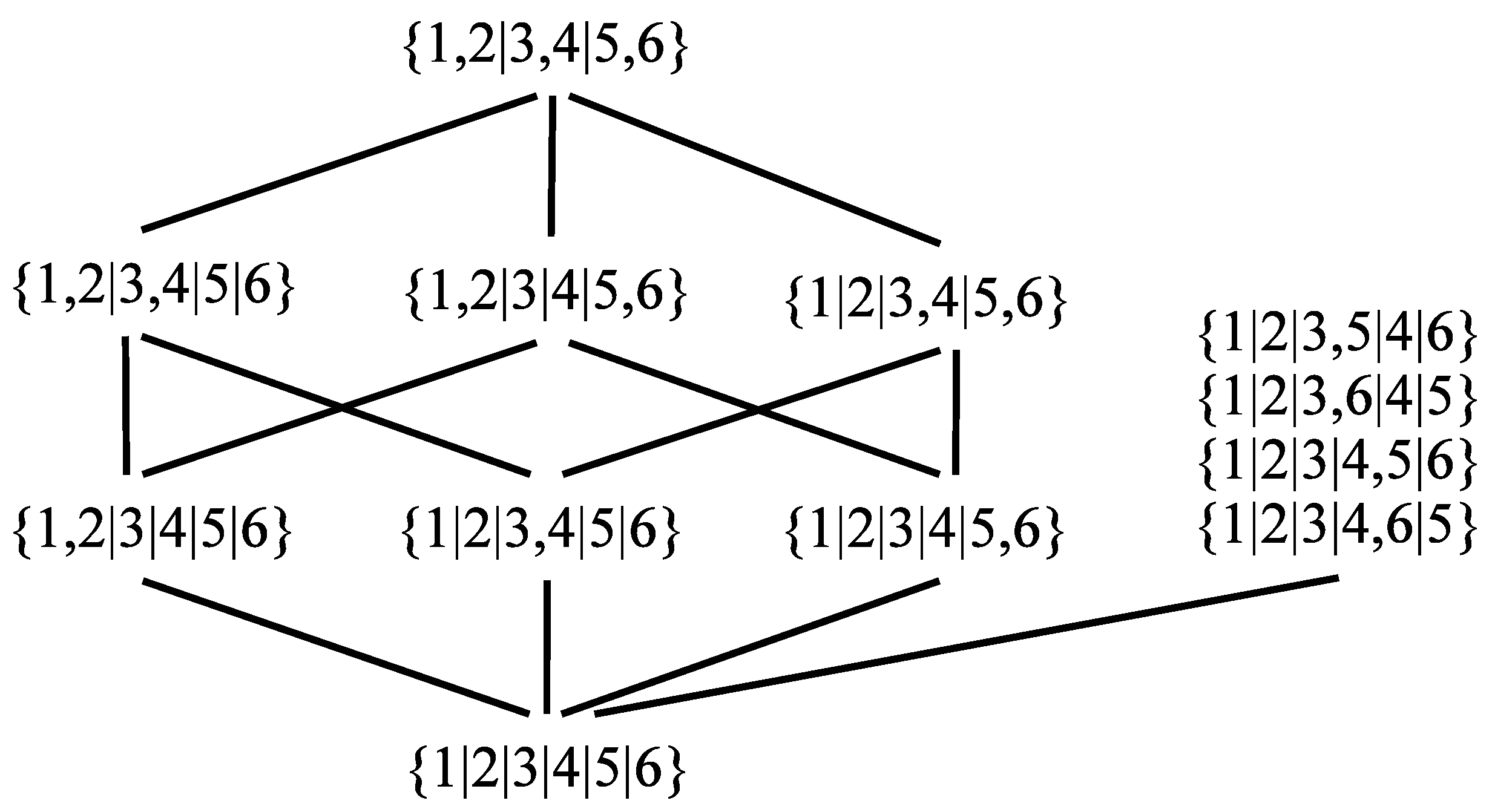
Definition 4.

(EE partition) Given a graph $G=(V,E)$, a partition $\{P_1,P_2,\cdots ,P_s\}$ of V is exploratory equivalent if there exists an ordered exploratory equivalent partition $\langle P_{i_1},P_{i_2},\dots ,P_{i_s}\rangle$ for a set of distinct indices $i_j\in \{1,\dots ,s\}$.

Notice that there can be many different EE partitions for a given graph. Figure 2 presents an example.

Every partition represents an equivalence relation, thuso the members of a partition are called classes rather than sets. Hence, the partition $\{1\mid 2\mid 3,4\mid 5\mid 6\}$ is composed of five equivalence classes and Vertices 3 and 4 are equivalent.

5.2. Maximum Exploratory Equivalence

As testified by the example in Figure 2, there may be many EE partitions for a particular graph. To be able to differentiate among partitions in terms of the pruning effectiveness of the search space, we provide a suitable measure. Furthermore, we also define a corresponding optimization problem that captures the main goal of our work, i.e., to speed up various exploration algorithms.

First, consider the monomorphism search problem described above. The size of the search space, i.e., the number of possible monomorphisms from the set A to the set B, is $\left(\genfrac{}{}{0pt}{}{\left|B\right|}{\left|A\right|}\right)\left|A\right|!$. Often, a search algorithm has to generate and process each and every of them. However, when the set A can be partitioned into the classes $P_1,P_2,\dots ,P_s$ containing equivalent elements (in the problem-specific sense), then the number of possibilities is reduced to

$$\left(\genfrac{}{}{0pt}{}{\left|B\right|}{\left|A\right|}\right)\frac{\left|A\right|!}{|P_1|!|P_2|!\dots |P_s|!}.$$

(8)

The reduction factor is thus given in the denominator as the product of factorials of set cardinalities. We often call this factor the score of a particular partition and use it as the objective in the maximum exploratory equivalent partition problem (MaxEE):

Definition 5.

(MaxEE) Given a graph $G=(V,E)$, find an EE partition $\{P_1,\dots ,P_s\}$ of V that maximizes the score

$$score\left(P\right)=\prod _{i=1}^s|P_i|!.$$

(9)

6. Computational Complexity

In this section, we tackle the computational complexity of the defined optimization problem. We first define an auxiliary problem, i.e., a verifier (VerifyEE) to check whether a given partition is a valid EE partition. We show that VerifyEE is GI-hard. Next, we define a natural decision version of MaxEE (we call it MaxEEDec) and reduce VerifyEE to MaxEEDec, demonstrating its GI-hardness.

Subsequently, we position VerifyEE more precisely; we show that the verifier belongs to the class of so-called intermediate problems, i.e., problems between $\mathcal{P}$ and $\mathcal{NP}$-complete. This is done by proving it to be at most as hard as the problem of finding the setwise stabilizer, which is currently also believed to be intermediate.

First, let us define the verifier problem.

Definition 6.

(VerifyEE) Given a graph $G=(V,E)$ and an ordered partition $\mathcal{P}=\{P_1,P_2,\dots ,P_s\}$ of the vertex set V, decide whether $\mathcal{P}$ is an EE partition of the graph G.

Theorem 1.

(GI-hardness)VerifyEEisGI-hard.

Proof. 

A pair of input graphs to the GI problem, $G=(V,E)$ and $H=(U,F)$ (without loss of generality, assume $\left|V\right|=\left|U\right|$), is transformed into the instance $(G^{\prime }=\langle V^{\prime },E^{\prime }\rangle ,\mathcal{P})$ of VerifyEE, where

$$V^{\prime }=V\cup U\cup \{v_G,v_H\},$$

$$\begin{array}{cc}\hfill E^{\prime }=& E\cup F\cup \{(v_G,v)\mid v\in V\}\cup \{(v_H,u)\mid u\in U\}\cup \left\{(v_G,v_H)\right\},\hfill \end{array}$$

(10)

and

$$\mathcal{P}=\left\{\{v_G,v_H\}\right\}\cup \{\left\{v\right\}\mid v\in V\cup U\}.$$

(11)

Now, we argue that $\mathcal{P}$ is an EE partition of $G^{\prime }$ iff G is isomorphic to H.

(⟹) If $(G^{\prime },\mathcal{P})$ is in VerifyEE, then there exists an automorphism on $G^{\prime }$ mapping $v_G$ to $v_H$. Furthermore, to preserve connectivity, all the vertices in V are mapped to the vertices in U, which is exactly an isomorphism between G and H.

(⟸) Let h denote an isomorphism from G to H. Construct an automorphism on $G^{\prime }$ that maps $v_G$ to $v_H$ and all the other vertices according to h and $h^{-1}$. Henceforth, $\{v_G,v_H\}$ is an EE class and $\mathcal{P}$ is an EE partition.  □

To establish the complexity of the MaxEE problem, we define a decision version of this problem.

Definition 7.

(MaxEEDec) Given a graph $G=(V,E)$ and an integer k, decide whether there exists an exploratory equivalent partition $\mathcal{P}$ with $score\left(\mathcal{P}\right)\ge k.$

We show the GI-hardness of this problem and the proof will require the following auxiliary lemma (i.e., we need to show that more refined partitions can only have smaller scores).

Lemma 1.

$\forall (k_1,k_2,\dots ,k_l),{\sum }_{i=1}^l{k}_i=n,k_i>0,l>1:n!>{\prod }_{i=1}^l{k}_i!$.

Proof. 

We need to prove this only for $l=2$, since any partition of n can be written as a sequence $n=k_1+k_2^{\prime }=k_1+k_2+k_3^{\prime }=\dots =k_1+k_2+\dots +k_{l-1}^{\prime }=k_1+k_2+\dots +k_{l-1}+k_l$. If we manage to prove the inequality for $l=2$, then the inequality follows for any $l\ge 2$.

The proof for $l=2$ is a simple observation:

$$n!=(1·2·3·\dots ·k_1)·((k_1+1)·(k_1+2)·\dots ·(k_1+k_2))>k_1!·k_2!,$$

(12)

since $(k_1+1)·(k_1+2)·\dots ·(k_1+k_2)>k_2!$ and $k_1>0$.  □

Theorem 2.

MaxEEDecisGI-hard.

Proof. 

We prove this by a reduction from VerifyEE, which is proven to be GI-hard above.

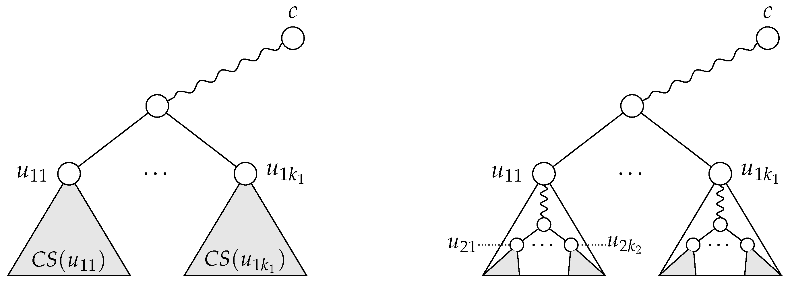
If we had labeled graphs, then we would simply color each $P_i$ with color i and ask whether such a labeled graph has an EE partition with score ${\prod }_{i=1}^s|P_i|!.$ However, since we are dealing with unlabeled graphs, we have to simulate the labels with gadgets that we add for each $P_i$.

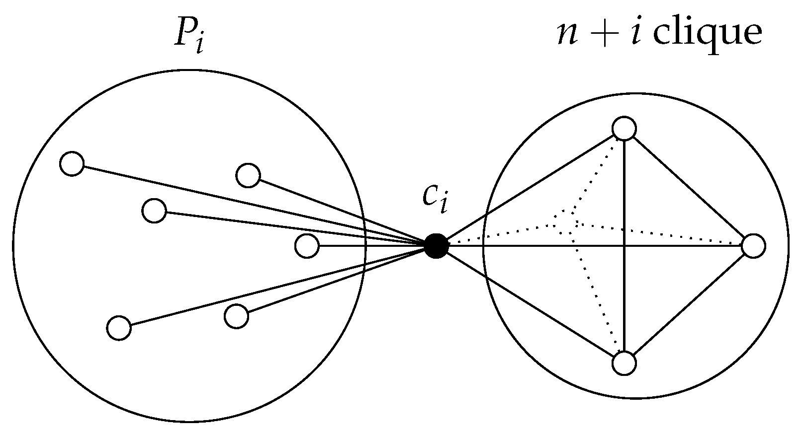
The reduction from VerifyEE (G, $\mathcal{P}$) to MaxEEDec ($G^{\prime }$, k) is as follows. We label each class $P_i\in \mathcal{P}$ by connecting each $v\in P_i$ to a gadget. Each class needs to have a distinct label, and we also need to make sure that each gadget cannot be mapped (by an automorphism) onto the rest of the graph. For each $P_i$, this gadget is a clique of $K_{n+i}$, which is connected to the set $P_i$ through a connecting vertex $c_i$. Each vertex in $P_i\cup K_{n+i}$ is connected to $c_i$. The sketch of this construction can be seen in Figure 3.

We can see that the vertices in each $K_{n+i}$ can only be isomorphic to each other and no other vertex. These vertices have a different degree than any vertex from the original graph G and also a different degree from any vertex in other cliques. The vertices $c_i$ are also unique (non-isomorphic to any other vertex), since they are always connected to non-isomorphic neighbors (those from $K_{n+i}$). Consequently, two vertices $u,v$ from G can be isomorphic only if they are in the same partition. These observations are helpful at the end of this proof.

Now, we also need to generate the appropriate score value:

$$k=\prod _{P_i\in P}|P_i|!(n+i)!.$$

(13)

We can now prove that:

$$\mathcal{P}\in EE\left(G\right)\iff \exists {\mathcal{P}}^{\prime }\in EE\left(G^{\prime }\right):score\left({\mathcal{P}}^{\prime }\right)\ge k.$$

(14)

(⟹) This direction is trivial, since the construction of $G^{\prime }$ does not impose any restrictions on isomorphisms in each $P_i$. Therefore, each $P_i$ is a valid EE set also in $G^{\prime }$. However, all vertices in each clique are also a valid EE set, thus we can construct the partition of $G^{\prime }$:

$${\mathcal{P}}^{\prime }=\bigcup _{P_i\in P}\left\{P_i,V\left(K_{n+i}\right),\left\{c_i\right\}\right\}.$$

(15)

The score of this partition is exactly k.

(⟸) We need to show that ${\mathcal{P}}^{\prime }$ must contain all the sets $P_i\in \mathcal{P}$. Because of the isomorphism restrictions we imposed by adding the gadgets, any EE partition on $G^{\prime }$ can only be a refinement of ${\mathcal{P}}^{\prime }$. Any refined EE partition ${\mathcal{P}}_{ref}^{\prime }$ has a strictly lower score than ${\mathcal{P}}^{\prime }$, which follows from Lemma 1.  □

The next goal of our complexity analysis is to demonstrate that the VerifyEE problem is (probably) not much harder than $\mathrm{GI}$. To do this, we reduce it to the problem of the setwise stabilizer of permutation groups, which is also $\mathrm{GI}$-hard [38], but widely believed not to be $\mathcal{NP}$-hard, for it is efficiently solvable in practice and exhibits similar properties as $\mathrm{GI}$.

The first step of our demonstration is to consider another problem, which is later used as the main ingredient for an algorithm for VerifyEE. In particular, we consider the problem of deciding the $cover(A,P)$ predicate for a given A and P. Notice that the necessary condition for A to cover P is that $\left|A\right|\ge \left|P\right|!$.

Lemma 2.

Given a group $A\subseteq S_n$ and a set $P\subseteq \{1,\cdots ,n\}$, deciding the $\mathit{cover}(A,P)$ predicate is polynomial-time reducible to calculating the setwise stabilizer $\mathit{SetStab}(A,P)$.

Proof. 

Let us restrict the set of permutations in A to those that stabilize the set P. This operation preserves all permutations that permute the elements of P. However, there might be more than $\left|P\right|!$ such permutations. Hence, we additionally restrict every generator of the group to the set P. More formally, we consider the set

$$A^{\prime }=\{a{|}_P\mid a\in \mathit{SetStab}(A,P)\}.$$

(16)

Now, we have

$$cover(A,P)\iff A^{\prime }=\mathrm{Sym}\left(P\right).$$

(17)

Notice that it is straightforward to compute ${a|}_P$, since every generator of the stabilizer group consists of two types of cycles: cycles where all elements belong to the set P, and those where none of the elements belongs to P.  □

Theorem 3.

VerifyEEis polynomial-time reducible to the problem of setwise stabilizer.

Proof. 

Following the definition of exploratory equivalence, we give an algorithm to compute VerifyEE (Algorithm 2). We omit checking that $P_1,P_2,\dots ,P_k$ is indeed a partition of a set of vertices.

$\mathit{PointStab}$ on Line 5 can be computed in polynomial time [39], so the problem further reduces to the cover problem, which is reducible by the previous lemma to $\mathit{SetStab}$.  □

Algorithm 2: Algorithm for computing VerifyEE.

7. Algorithms

Due to the complexity results in the previous section, we do not focus on trying to find an optimal solution for the general MaxEE problem. Instead, we first describe a (relatively) time-efficient heuristic algorithm, making it more suitable for potential practical applications. Subsequently, we demonstrate that, by reducing the problem to trees, we can find an optimal solution in polynomial time.

Since we are dealing with a problem that is currently speculated to be harder than $\mathcal{NP}$, we focus on finding a good heuristic method whose time complexity remains feasible.

7.1. Heuristics for General Graphs

Here, we present a greedy heuristic algorithm for solving the MaxEE problem. The algorithm is based on the recursive procedure given in Algorithm 3. The procedure receives as an input a current permutation group A as well as a current (partial) EE partition $\{P_1,P_2,\dots ,P_k\}$, where the set $P_k$ is not finalized yet and can be extended with additional elements. On the other hand, the sets $P_i$ with $1\le i<k$ are final; additionally, the group A is pointwise stabilized to all the elements in these sets. The algorithm starts with $A=\mathrm{Aut}\left(G\right)$ and an empty partial partition.

Algorithm 3: Heuristics for the MaxEE problem.

The halting condition for this algorithm is satisfied when the automorphism group stabilized to all the elements in the partial partition contains only the trivial automorphism. In this case, the current partition is the final solution (Line 4).

When the partial partition is empty ($k=0$), $P_1$ becomes a pair of elements with the best potential for expansion (Line 7). Otherwise, in each recursive step, a choice between two possibilities is made (Line 12):

• The set $P_k$ is augmented by a single element (the call to augment computes the best candidate for augmentation; see Lines 10 and 13).
• $P_k$ is finalized, a new pair of elements is selected as the set $P_{k+1}$, and A is pointwise stabilized on $P_k$ (bestEEPair returns the pair of elements that exhibit the best potential; see Lines 11 and 15).

This choice is done greedily, using the following criterion

$$\phi (A,P)=\left|P\right|!·\left|notFixed\right(\mathit{PointStab}(A,P)\left)\right|!,$$

(18)

which estimates the potential of a set P in a group A. Here, the $\left|P\right|!$ factor comes from the MaxEE objective function, and

$$notFixed\left(A\right)=\{i\mid \exists a\in A:a(i)\ne i\}$$

(19)

consists of positions not yet fixed.

Now, consider the functions bestEEPair and augment (Algorithm 4). In the former, to select the best pair of vertices in a given group A, we first find candidate pairs using the orbits of the group (Line 2). Notice that a pair of vertices in the same orbit trivially satisfies the $\mathit{cover}$ predicate. Nevertheless, this is basically an optimization, for the set of all pairs could be used instead. From such a candidate set, the best pair is chosen (Line 3) using the potential criterion defined above.

Algorithm 4: The definition of two auxiliary functions

A similar idea is behind augmenting an existing EE set P. The candidates are the elements i in the same orbit as the elements of P, and the set $P\cup \left\{i\right\}$ also has to be exploratory equivalent. From this set of candidates, the element with the highest potential criterion function $\phi$ is selected.

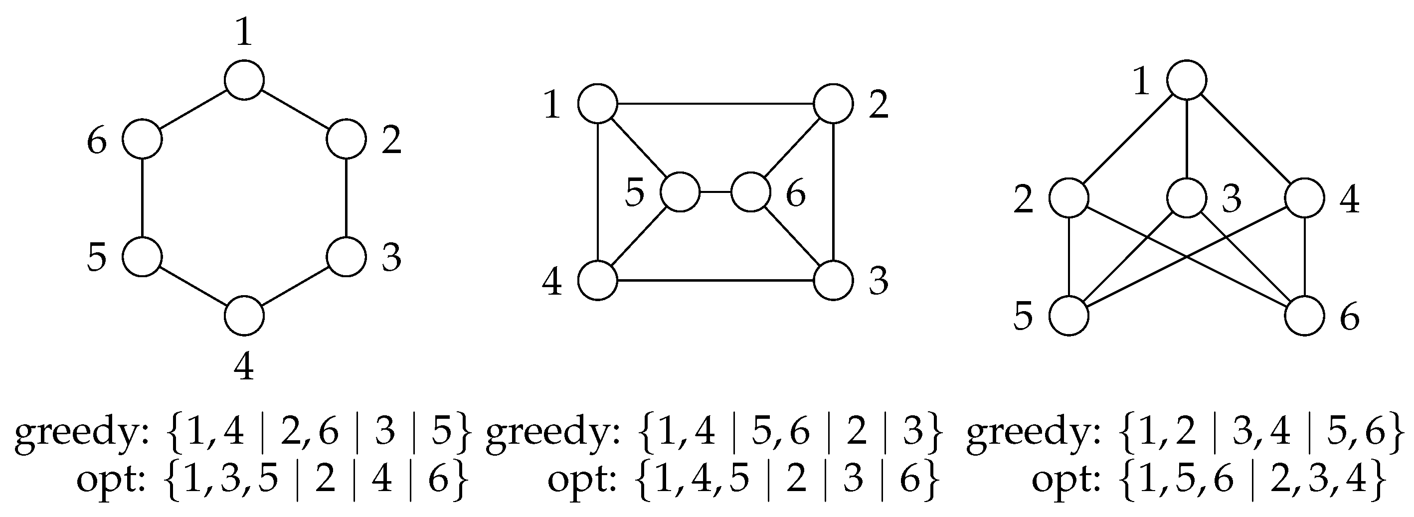
On certain input instances, the algorithm finds suboptimal partitions. The smallest such inputs are the three six-vertex graphs shown in Figure 4. Nevertheless, we present a small experimental evaluation in Section 9, showing that in most cases the heuristics are indeed highly successful in finding an optimal solution.

Time Complexity

The time complexity of the described heuristics is dominated by the complexity of the setwise stabilizer. All the other building blocks of this algorithm are of polynomial time complexity. The time complexity of the set stabilizer is still exponential in the classical sense, but that does not do the problem justice. A more informative fact about the set stabilizer problem is that it is not NP-complete and, like GI, this problem is easy on the vast majority of practical instances (for a more detailed description of the context of the set-stabilizer problem, see [40]). This is what makes it a practical option for our heuristics and we could see this almost polynomial behavior also in our practical experiments, which is discussed in Section 9.

7.2. Exact Algorithm on Trees

Since the MaxEE problem is unlikely to be solvable in polynomial time for general graphs, we restrict our attention to trees. We show that for an arbitrary tree, the MaxEE problem can be solved by a polynomial-time algorithm.

To begin with, let us introduce some tree-related concepts. For a given tree $T=(V,E)$, the distance between vertices u and v, denoted $d(u,v)$, is the number of edges on the (unique) path from u to v. The height of a tree T, $h\left(T\right)$, is the maximum distance between a pair of vertices, i.e., $h\left(T\right)={max}_{\{u,v\}\subseteq V}d(u,v)$. The neighborhood subtree of a vertex u at a distance d, denoted ${\mathit{NS}}_d\left(u\right)$, is the subtree of T composed of all vertices whose distance from u is at most d. A vertex u can be automorphically mapped (a vertex u can be “automorphically mapped” to a vertex v if there exists an automorphism that maps u to v.) to a vertex v only if ${\mathit{NS}}_d\left(u\right)\simeq {\mathit{NS}}_d\left(v\right)$ for all $d\ge 0$.

The eccentricity of a vertex u, denoted $e\left(u\right)$, is the maximum distance between u and any other vertex in the tree, i.e., $e\left(u\right)={max}_{v\in V}d(u,v)$. A center of the tree is a vertex with minimum eccentricity. Let $e=e\left(c\right)$, where c is a center of the tree.

Lemma 3.

Every tree has either one or two centers. In the latter case, the centers are connected by an edge.

The proof can be found in [41]. We will denote the centers by $c_1$ and $c_2$, allowing for the possibility that $c_1=c_2=c$.

Let $\mathcal{E}(u,v)$ denote the set of edges on the path from u to v. For a tree T, the centrifugal subtree of a vertex $u\notin \{c_1,c_2\}$, denoted $\mathit{CS}\left(u\right)$, is a subtree of T composed of all vertices v such that $\mathcal{E}(u,v)\cap (\mathcal{E}(u,c_1)\cup \mathcal{E}(u,c_2))=\varnothing$. For a tree with a single center c, $\mathit{CS}\left(c\right)=T$; for a tree with distinct centers $c_1$ and $c_2$, the tree $\mathit{CS}\left(c_i\right)$ (for $i\in \{1,2\}$) is induced by the vertex set $\{v\in V\mid (c_1,c_2)\notin \mathcal{E}(c_i,v)\}$

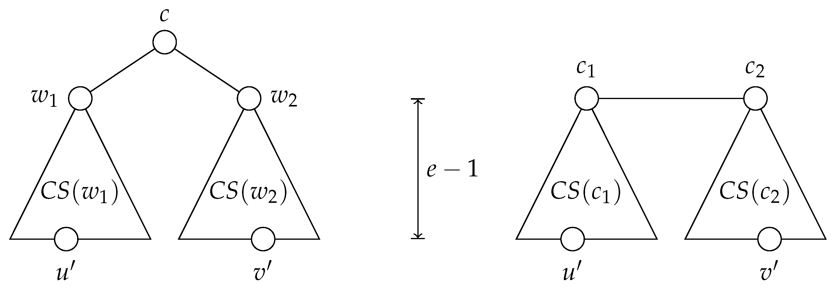
Lemma 4.

(1) If a tree has a single center c and if $e\ge 1$, there exist distinct vertices $u^{\prime }$ and $v^{\prime }$ such that $d(c,u^{\prime })=d(c,v^{\prime })=e$ and $\mathcal{E}(c,u^{\prime })\cap \mathcal{E}(c,v^{\prime })=\varnothing$. (2) If a tree has distinct centers $c_1$ and $c_2$ and if $e\ge 2$, there exist distinct vertices $u^{\prime }$ and $v^{\prime }$ such that $d(c_1,u^{\prime })=d(c_2,v^{\prime })=e-1$ and $\mathcal{E}(c_1,u^{\prime })\cap \mathcal{E}(c_2,v^{\prime })=\varnothing$.

Proof. 

Let us begin with Property (1). First, if $e\ge 1$, the center of the tree has at least two neighbors (say, $w_1$ and $w_2$); otherwise, it would not be the sole center or a center at all. Now, let us show that the trees $\mathit{CS}\left(w_1\right)$ and $\mathit{CS}\left(w_2\right)$ have an equal height. If $h\left(\mathit{CS}\left(w_1\right)\right)\le h\left(\mathit{CS}\left(w_2\right)\right)-2$, then $w_2$ has a smaller eccentricity than c, thus c cannot be a center. If $h\left(\mathit{CS}\left(w_1\right)\right)=h\left(\mathit{CS}\left(w_2\right)\right)-1$, then c is not the sole center of the tree; $w_2$ is another. Since the cases $h\left(\mathit{CS}\left(w_2\right)\right)\le h\left(\mathit{CS}\left(w_1\right)\right)-2$ and $h\left(\mathit{CS}\left(w_2\right)\right)=h\left(\mathit{CS}\left(w_1\right)\right)-1$ are symmetric, it follows that $h\left(\mathit{CS}\left(w_1\right)\right)=h\left(\mathit{CS}\left(w_2\right)\right)=e\left(w_1\right)=e\left(w_2\right)=e-1$. Let us pick vertices $u^{\prime }\in \mathit{CS}\left(w_1\right)$ and $v^{\prime }\in \mathit{CS}\left(w_2\right)$ such that $d(w_1,u^{\prime })=d(w_2,v^{\prime })=e-1$ (see Figure 5, left). The distances $d(c,u^{\prime })$ and $d(c,v^{\prime })$ are both equal to e, and, since the trees $\mathit{CS}\left(w_1\right)$ and $\mathit{CS}\left(w_2\right)$ are disjoint, we also have $\mathcal{E}(c,u^{\prime })\cap \mathcal{E}(c,v^{\prime })=\varnothing$.

As for Property (2), note that $h\left(\mathit{CS}\left(c_1\right)\right)=h\left(\mathit{CS}\left(c_2\right)\right)$: if $h\left(\mathit{CS}\left(c_1\right)\right)$ were smaller than $h\left(\mathit{CS}\left(c_2\right)\right)$, then $c_1$ could not be a center, and symmetrically for the case $h\left(\mathit{CS}\left(c_2\right)\right)<h\left(\mathit{CS}\left(c_1\right)\right)$. Given that $h\left(\mathit{CS}\left(c_1\right)\right)=h\left(\mathit{CS}\left(c_2\right)\right)=e-1$, there is a vertex $u^{\prime }$ at a distance $e-1$ from $c_1$ and a vertex $v^{\prime }$ at the same distance from $c_2$ (see Figure 5, right). Since the trees $\mathit{CS}\left(c_1\right)$ and $\mathit{CS}\left(c_2\right)$ are disjoint, $\mathcal{E}(c_1,u^{\prime })\cap \mathcal{E}(c_2,v^{\prime })=\varnothing$.  □

Lemma 5.

If vertices u and v belong to the same orbit of the given tree, then all of the following hold:

(1) 

If the tree has a single center, then $d(u,c)=d(v,c)$.

(2) 

If the tree has two distinct centers, then $d(u,c_1)=d(v,c_1)$ if $d(u,v)$ is even and $d(u,c_1)=d(v,c_2)$ if $d(u,v)$ is odd.

(3) 

$\mathit{CS}\left(u\right)\simeq \mathit{CS}\left(v\right)$.

Proof. 

For trees consisting of at most two vertices, the lemma can easily be verified. We may thus assume that the tree has at least three vertices.

(1)

By Lemma 4, a tree with a single center c contains distinct vertices $u^{\prime }$ and $v^{\prime }$ such that $d(c,u^{\prime })=d(c,v^{\prime })=e$ and the paths from c to $u^{\prime }$ and from c to $v^{\prime }$ are disjoint. Without loss of generality, we may assume that $d(u,c)<d(v,c)$ and that the vertex v does not lie on the path from c to $u^{\prime }$ (if it does, we can swap $u^{\prime }$ and $v^{\prime }$). The distance from v to $u^{\prime }$ is $D=d(v,c)+d(c,u^{\prime })=d(v,c)+e$. However, the most distant vertex from u can be at most $d(u,c)+e\le D-1$ edges away from u. Therefore, the tree ${\mathit{NS}}_D\left(v\right)$ has more vertices than ${\mathit{NS}}_{D-1}\left(v\right)$, but the tree ${\mathit{NS}}_D\left(u\right)$ is the same as ${\mathit{NS}}_{D-1}\left(u\right)$. Consequently, u and v cannot be automorphically mapped to each other and hence cannot belong to the same orbit.

(2)

Lemma 4 ensures the existence of vertices $u^{\prime }$ and $v^{\prime }$ such that $d(c_1,u^{\prime })=d(c_2,v^{\prime })=e-1$ and the paths from $c_1$ to $u^{\prime }$ and from $c_2$ to $v^{\prime }$ are disjoint. Let the vertices u and v belong to the same orbit, and let us assume that $d(u,v)$ is even. If u and v belong to the centrifugal subtrees of different centers (say, u belongs to $\mathit{CS}\left(c_1\right)$ and v to $\mathit{CS}\left(c_2\right)$), then $d(u,c_1)\ne d(v,c_2)$, contradicting our assumption that u and v are both part of the same orbit: $d(u,c_1)<d(v,c_2)$ implies that the vertex $u^{\prime }$ is located $d(v,c_2)+e$ edges away from v but there is no such vertex at the same distance from u, and a symmetrical conclusion follows from $d(u,c_1)>d(v,c_2)$. Therefore, an even value of $d(u,v)$ means that u and v both belong to either $\mathit{CS}\left(c_1\right)$ or $\mathit{CS}\left(c_2\right)$ and (by applying a distance-based argument once again) that $d(u,c_1)=d(v,c_1)$. In a similar fashion, we can show that an odd value of $d(u,v)$ means that u belongs to $\mathit{CS}\left(c_1\right)$ and v to $\mathit{CS}\left(c_2\right)$ (or the other way around) and that $d(u,c_1)=d(v,c_2)$.

(3)

If the subtrees $\mathit{CS}\left(u\right)$ and $\mathit{CS}\left(v\right)$ are non-isomorphic, there exists some distance d at which the neighborhood subtrees of u and v are non-isomorphic. Therefore, no automorphism can map u to v and vice versa, and so these two vertices do not belong to the same orbit.

 □

The following lemma specifies a sufficient condition for a vertex set partition to be exploratory equivalent.

Lemma 6.

An ordered partition $\mathcal{P}=\langle P_1,\dots ,P_s\rangle$ of the vertex set V of a given tree T is exploratory equivalent if all of the following conditions hold:

(1) 

for each $i\in \{1,\dots ,s\}$, all vertices in $P_i$ belong to the same orbit of T;

(2) 

for each $i\in \{2,\dots ,s\}$ and for all pairs $u,v\in P_i$, we have $d(u,v)=2$;

(3) 

either (i) $d(u,v)=2$ for all pairs $u,v\in P_1$ or (ii) $P_1=\{c_1,c_2\}$ and $c_1\ne c_2$;

(4) 

if $i\ne j$ and there exists a vertex $v\in P_i$ such that $P_j\subseteq \mathit{CS}\left(v\right)$, then $j>i$.

Proof. 

To verify that the partition $\mathcal{P}$ is exploratory equivalent, we first have to show that the automorphism group of the tree, $\mathrm{Aut}\left(T\right)$, covers the set $P_1$. By Lemma 5, the fact that all vertices in $P_1$ belong to the same orbit implies that they are located at the same distance from the center(s) and that their centrifugal subtrees are isomorphic. If $c_1\ne c_2$, $P_1=\{c_1,c_2\}$, and $\mathit{CS}\left(c_1\right)\simeq \mathit{CS}\left(c_2\right)$, then $\mathrm{Aut}\left(T\right)$ clearly covers $P_1$, since $c_1$ can be automorphically mapped to $c_2$ and vice versa. If, however, all vertices of $P_1$ are located at the pairwise distance of 2, then they are connected with a common neighbor, in addition to having isomorphic centrifugal subtrees (see Figure 6, left). Consequently, the vertices of $P_1$ can be automorphically mapped to each other in all possible ways, i.e., the set $\mathrm{Aut}\left(T\right)$ contains an automorphism for all $|P_1|!$ permutations of $P_1$. In other words, $\mathrm{Aut}\left(T\right)$ covers $P_1$.

Now, let us pointwise-stabilize the set $\mathrm{Aut}\left(T\right)$ with respect to the set $P_1$ and check whether the reduced set of automorphisms covers $P_2$. The pointwise stabilization can be interpreted as making the vertices in $P_1$ distinguishable (e.g., by assigning distinct colors or labels to them). After this operation, can the vertices of $P_2$ still be automorphically mapped to each other? Condition (4) in the lemma allows for two possibilities: (i) the set $P_2$ is disjoint from all centrifugal subtrees of the vertices in $P_1$ (in which case the pointwise stabilization with respect to $P_1$ has absolutely no impact on $P_2$); and (ii) the set $P_2$ is part of the centrifugal subtree of some vertex in $P_1$. In the latter case, as depicted in Figure 6 (right), the vertices of $P_2$ can still be automorphically mapped to each other in every possible way, since they are connected to the same neighbor and since their centrifugal subtrees remain unaffected by the pointwise stabilization. In the same way, we can argue that the set $P_3$ remains covered after pointwise-stabilizing the current set of automorphisms with respect to the set $P_2$. Since the same logic applies all the way to $P_s$, we can conclude that the partition $\mathcal{P}$ is exploratory equivalent.  □

The next lemma forms the basis for an algorithm to find a maximum EE partition of a given tree.

Theorem 4.

For any tree, there exists a maximum EE partition that satisfies Conditions (1)–(3) from Lemma 6.

Proof. 

Every EE partition has to satisfy Condition (1); if vertices $v_1$, …, $v_k$ do not belong to the same orbit, they cannot be automorphically mapped to each other and hence cannot possibly constitute a class in an EE partition.

As for Conditions (2) and (3), let $P=\{v_1,\dots ,v_k\}$ be a class in a maximum EE partition $\mathcal{P}$, and let $d(v_i,v_j)>2$ for some i and j. For the time being, let us assume that the tree has only one center, i.e., $c=c_1=c_2$. Since the vertices in P belong to the same orbit, Lemma 5 ensures that $d(v_1,c)=\dots =d(v_k,c)$ and $\mathit{CS}\left(v_1\right)\simeq \dots \simeq \mathit{CS}\left(v_k\right)$. 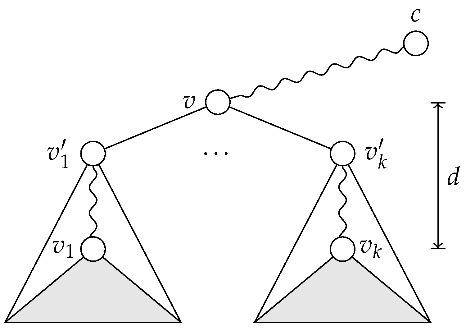Now, let v be the vertex with the property $d(v_1,v)=\dots =d(v_k,v)=d$ that minimizes the distance d, and let $v_i^{\prime }$, for $i\in \{1,\dots ,k\}$, be the neighbor of v on the path from v to $v_i$ (Figure 7). We claim that the partition ${\mathcal{P}}^{\prime }$ obtained by replacing the set P with the set $P^{\prime }=\{v_1^{\prime },\dots ,v_k^{\prime }\}$ (and adding the vertices $v_1$, …, $v_k$ as singletons) is still a maximum EE partition. First, if the automorphism group of the tree covers P, it also covers $P^{\prime }$, since an automorphism that maps $v_i$ to $v_j$ maps the entire centrifugal subtree of $v_i^{\prime }$ to that of $v_j^{\prime }$ (and $v_i^{\prime }$ itself to $v_j^{\prime }$). Second, in the original partition ($\mathcal{P}$), the vertices $v_1^{\prime }$, …, $v_k^{\prime }$ had to occur as singletons; otherwise, $\mathcal{P}$ would not be EE, since an automorphism mapping $v_i^{\prime }$ to $v_j^{\prime }$ also maps $v_i$ to $v_j$. Therefore, the score of ${\mathcal{P}}^{\prime }$ is the same as that of $\mathcal{P}$, and if $\mathcal{P}$ is maximum, so is ${\mathcal{P}}^{\prime }$. To see that the partition ${\mathcal{P}}^{\prime }$ remains to be EE, consider that the replacement of the constituent class P with the set $P^{\prime }$ could rule out only classes composed of vertices on the paths from $v_1^{\prime }$, …, $v_k^{\prime }$ to $v_1$, …, $v_k$. However, in the partition $\mathcal{P}$, these vertices could only occur as singletons, since an automorphism that interchanges $v_i$ with $v_j$ interchanges the entire path from $v_i^{\prime }$ to $v_i$ with the path from $v_j^{\prime }$ to $v_j$. Therefore, every EE class containing vertices at a pairwise distance greater than 2 can be replaced by one where the pairwise distance is exactly 2.

If the tree has two distinct centers and if $d=d(v_1,c_1)=\dots =d(v_k,c_1)$ is even, the set $P^{\prime }=\{v_1^{\prime },\dots ,v_k^{\prime }\}$ can be constructed from the set $P=\{v_1,\dots ,v_k\}$ in exactly the same way as in the single-center case. However, if d is odd, then P contains exactly two vertices (say, u and v), and $d(u,c_1)=d(v,c_2)$. In a similar manner as above, we can replace the class $P=\{u,v\}$ with the class $P^{\prime }=\{c_1,c_2\}$ in the partition $\mathcal{P}$, and the resulting partition is still a maximum EE partition.  □

Incidentally, note that the classes in an unordered maximum EE partition that fulfills Conditions (1)–(3) from Lemma 6 can always be ordered in such a way that the resulting ordered partition fulfills Condition (4), too.

We have seen that the search for a maximum EE partition of a given tree can be restricted to those partitions where all constituent classes consist solely of vertices at a pairwise distance of at most 2. Since every class in an EE partition has to be a subset of some orbit, an algorithm for finding a maximum EE partition can easily be devised: start with the set of orbits of the given tree ($O_1$, …, $O_r$), and partition each orbit $O_i$ into sets $P_{i1}$, …, $P_{i{k}_i}$ such that for each $j\in \{1,\dots ,k_i\}$ the distance between each pair of vertices in $P_{ij}$ is at most 2. The sets $P_{ij}$ jointly form a maximum EE partition of the input tree. This procedure is presented as Algorithm 5.

Algorithm 5: A polynomial-time algorithm to find a maximum EE partition for a tree T.

The set of orbits of the input tree can be produced in time $O\left(n\right)$ [42]. The rest of the algorithm can be performed in time $O\left(n^2\right)$; in the worst case, the algorithm has to determine for each pair of tree vertices whether the distance between them is equal to 2. Therefore, the entire algorithm runs in time $O\left(n^2\right)$.

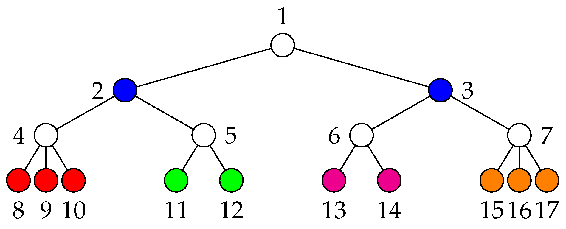
For example, the tree in Figure 8 has the following orbits: $O_1=\left\{1\right\}$, $O_2=\{2,3\}$, $O_3=\{4,7\}$, $O_4=\{5,6\}$, $O_5=\{8,9,10,15,16,17\}$, and $O_6=\{11,12,13,14\}$. Algorithm 5 splits the orbits $O_3$, $O_4$, $O_5$, and $O_6$, each into two sets. The resulting maximum EE partition is thus $\{1\mid 2,3\mid 4\mid 5\mid 6\mid 7\mid 8,9,10\mid 11,12\mid 13,14\mid 15,16,17\}$.

7.3. Exact Algorithm on Cycles

Cycles deserve special attention because they represent a frequent counterexample for the proposed heuristic algorithm (Section 7.1) and because they belong to a class of graphs for which maximum EE partitions do not capture the entire set of automorphisms (Section 9). Nevertheless, it is possible to identify a set of rules that determine a maximum EE partition for any given cycle. In what follows, the n-cycle (with $n\ge 3$) is a graph composed of vertices 1, 2, …, n and edges $(1,2)$, $(2,3)$, …, $(n-1,n)$, $(n,1)$. Note that the automorphism group of the n-cycle comprises the automorphisms $(i$, $i+1$, …, n, 1, 2, …, $i-1)$ and $(i$, $i-1$, …, 1, n, $n-1$, …, $i+1)$ for all $i\in \{1,\dots ,n\}$. A cycle with an even (odd) number of vertices is also called an even cycle (an odd cycle, respectively).

To simplify notation in the following proofs, let $m_0\left(k\right)=kmodn$, and let

$$m\left(k\right)=\left\{\begin{array}{cc}{m}_0\left(k\right)+n\hfill & \mathrm{if}{m}_0\left(k\right)<0,\hfill \\ n\hfill & \mathrm{if}{m}_0\left(k\right)=0,\hfill \\ m_0\left(k\right)\hfill & \mathrm{if}{m}_0\left(k\right)>0\hfill \end{array}\right.$$

(20)

for a fixed positive integer n and an arbitrary integer k. Note that $m\left(k\right)=k$ for $k\in \{1,\dots ,n\}$ and $m(k+in)=m\left(k\right)$ for an arbitrary integer i.

Lemma 7.

In an odd n-cycle, an automorphism that swaps the vertices u and v fixes the vertex $(u+v)/2$ if $u+v$ is even and $m\left(\right(u+v+n)/2)$ if $u+v$ is odd.

Proof. 

Without loss of generality, we may assume that $u<v$. If $u+v$ is even, the path $\langle u$, $m(u+1)$, $m(u+2)$, …, $m(v-2)$, $m(v-1)$, $v\rangle$ contains an odd number of vertices. Consequently, an automorphism that swaps the vertices u and v also swaps the vertices $m(u+i)$ and $m(v-i)$ for an arbitrary i. The vertex $m(u+(v-u)/2)=m(v-(v-u)/2)=m\left(\right(u+v)/2)=(u+v)/2$, which lies in the middle of the path, is swapped with itself, i.e., kept fixed.

If $u<v$ and $u+v$ is odd, the path $\langle u$, $m(u-1)$, $m(u-2)$, …, $m(v+2)$, $m(v+1)$, $v\rangle$ (e.g., $\langle 3,2,1,7,6\rangle$ if $n=7$, $u=3$, and $v=6$) contains an odd number of vertices. An automorphism that swaps u and v also swaps the vertices $m(u-i)$ and $m(v+i)$ for an arbitrary i. For $i=(u-v-n)/2$, we obtain $m(u-i)=m(v+i)=m\left(\right(u+v+n)/2)$, thus this vertex is fixed.  □

Lemma 8.

In an even n-cycle, an automorphism that swaps the vertices u and v fixes no vertices if $u+v$ is odd and the vertices $(u+v)/2$ and $m\left(\right(u+v+n)/2)$ if $u+v$ is even.

Proof. 

As in the proof of Lemma 7, let $u<v$. If $u+v$ is odd, then both the path $\langle u$, $m(u+1)$, …, $m(v-1)$, $v\rangle$ and the path $\langle u$, $m(u-1)$, …, $m(v+1)$, $m\left(v\right)\rangle$ contain an even number of vertices. In this case, swapping the vertices u and v does not fix any vertex; we cannot choose an integer i such that $m(u+i)=m(v-i)$. However, if $u+v$ is even, both paths contain an odd number of vertices. The automorphism fixes the midpoints of the two paths, i.e., the vertices $(u+v)/2$ and $m\left(\right(u+v+n)/2)$.  □

Lemma 9.

A maximum EE partition of an odd cycle contains exactly one nonsingleton class, and that class consists of at most three vertices.

Proof. 

By Lemma 7, an automorphism that swaps a pair of vertices u and v fixes exactly one vertex. Consequently, a maximum EE partition contains at most one nonsingleton class, and that class consists of at most three vertices: the vertices u and v and, as shown below, in some cases also the vertex fixed by the automorphism that swaps u and v. However, in any cycle, any two vertices can be automorphically mapped to each other, which means that a maximum EE partition contains exactly one nonsingleton class.  □

Lemma 10.

In any $\left(3k\right)$-cycle, the partition ${\mathcal{P}}_3=\{k,2k,3k\mid singletons\}$ is exploratory equivalent. (If a partition of a set P is written as $\mathcal{P}=\{P_1\mid \dots \mid P_s\mid singletons\}$, then all elements from the set $P\backslash (P_1\cup \dots \cup P_s)$ occur in $\mathcal{P}$ as singletons.)

Proof. 

The partition ${\mathcal{P}}_3$ is EE because the automorphism group of the $\left(3k\right)$-cycle covers all $3!$ permutations of the set $\{k$, $2k$, $3k\}$, as shown in

Table 1. The cover of all $3!$ permutations of the set $\{k,2k,3k\}$.

.  □

Lemma 11.

For an odd n-cycle where n is not divisible by 3, a maximum EE partition is $\{1,2\mid singletons\}$.

Proof. 

By Lemma 9, the sole nonsingleton set of a maximum EE partition for an odd cycle has at most three vertices. However, for an automorphism group to cover a set of three vertices (as is the case in the proof of Lemma 10), these vertices have to be evenly spaced along the cycle. This is only possible if the number of vertices of the cycle is divisible by 3.  □

Lemma 12.

For a $\left(2k\right)$-cycle, a maximum EE partition is $\{1,3\mid 2,k+2\mid singletons\}$ if k is not divisible by 3 and $\{2k/3,4k/3,6k/3\mid singletons\}$ if it is.

Proof. 

Since the sum of $u=1$ and $v=3$ is even, Lemma 8 guarantees that the automorphism that swaps the vertices u and v fixes both the vertex $w=(u+v)/2=2$ and the vertex $z=(u+v+2k)/2=k+2$. The partition $\{1,3\mid 2,k+2\mid \mathrm{singletons}\}$ is thus a candidate EE partition, and it can be readily verified that it is indeed EE: by pointwise-stabilizing the initial set of automorphisms with respect to the set $\{2,k+2\}$, we obtain a set of automorphisms that still covers the set $\{1,3\}$ (the corresponding ordered EE partition is hence $\langle 2,k+2\mid 1,3\mid \mathrm{singletons}\rangle$). If k is not divisible by 3, this partition has the greatest possible score ($2!2!=4$). In the opposite case, the alternative EE partition $\{2k/3,4k/3,6k/3\mid \mathrm{singletons}\}$ has a greater score and is hence maximum.  □

The results given above can be summarized as follows:

Theorem 5.

A maximum EE partition for an n-cycle is:

• $\{n/3,2n/3,n\mid singletons\}$ if $n=3k$;
• $\{1,3\mid 2,n/2+2\mid singletons\}$ if $n=6k-4$ or $n=6k-2$; and
• $\{1,2\mid singletons\}$ if $n=6k-5$ or $n=6k-1$.

8. Application to the Subgraph Isomorphism Problem

As mentioned in the first paragraph of the Introduction, our approach was initially inspired by the subgraph isomorphism problem, which seeks to identify the occurrences of a pattern graph G in a host graph H. This problem can be readily applied to fields such as chemistry, where one may look for specific functional groups within a large molecule, or network analysis, where searching for particular community patterns might be of interest. Given the ever-increasing number, size, and impact of social networks in today’s world, we can be sure that the applicability of the subgraph isomorphism search problem may only grow.

In this section, we consider the version of the subgraph isomorphism problem in which the goal is to enumerate all occurrences of a pattern graph in a host graph. As mentioned in Section 4, the subgraph isomorphism problem is a special case of a more general monomorphism search problem. Therefore, if the pattern graph has at least one non-identity automorphism and hence at least one nonsingleton class in its maximum exploratory equivalent partition, we can use Algorithm 1 to speed up the search.

Algorithm 1 is independent of the subgraph isomorphism search method. It only assumes that the search method constructs (partial and total) monomorphisms between the pattern graph and the host graph (which, by definition, is what every search algorithm does) but does not require anything else. The search algorithm may produce monomorphisms in any order.

We applied Algorithm 1 to a search method based on search plans [2,43]. Search plans were used, for instance, to perform subgraph isomorphism search in the graph grammar parser of Rekers and Schürr [2,3]. A search plan of a given pattern graph G is a sequence of instructions for a systematic traversal of the vertices and edges of an occurrence of G in an arbitrary host graph H. The first instruction of a search plan always takes the form $\left[u\right]$ and is read as “pick an arbitrary vertex $w\in V_H$ and map it to the vertex $u\in V_G$ (i.e., establish $h\left(u\right)=w$)”. All other instructions take either the form $[u\to v]$ (“start at the vertex already mapped to $u\in V_G$, visit one of its as-yet unvisited neighbors together with the edge connecting the two vertices, and map the neighbor to the vertex $v\in V_G$”) or the form $[u?v]$ (“verify the existence of an edge between the vertices already mapped to u and v, and visit that edge”). Note that any sequence of instructions that visits all vertices and edges constitutes a valid search plan.

A naive subgraph isomorphism search algorithm simply tries to carry out each instruction in all possible ways using backtracking. It thus finds all occurrences of G and H, but each occurrence is discovered $\left|\mathrm{Aut}\right(G\left)\right|$ times. To reduce the number of discoveries, we employ exploratory equivalence, as dictated by Algorithm 1. For each nonsingleton class $\{u_1$, …, $u_k\}$ in the optimal EE partition $\mathcal{P}$ of G, we impose the constraint $h\left(u_1\right)<\dots <h\left(u_k\right)$; the search algorithm is allowed to produce and extend only those partial and total monomorphisms that satisfy this restriction. In this way, the algorithm will still find all occurrences of G in H, but the number of discoveries will be reduced by a factor of $\mathit{score}\left(\mathcal{P}\right)$.

For instance, if we were searching for the occurrences of the graph $C_4$ (

Table 2. Pattern graphs used in our experiments. In the same fashion as in Figure 8, different colors indicate different equivalence classes in the optimal EE partition, and the uncolored vertices constitute the singleton classes.

Pattern Graph (G)	${\mathit{L}}_4$	${\mathit{C}}_4$	${\mathit{K}}_4$
Structure and maximum EE partition
$\left|\mathrm{Aut}\right(G\left)\right|$	2	8	24
Score of max. EE part.	2	4	24
Search plan used in the experiments	$[1]$ $[1\to 2]$ $[2\to 3]$ $[3\to 4]$	$[1]$ $[1\to 2]$ $[2\to 3]$ $[3\to 4]$ $[1?4]$	$[1]$ $[1\to 2]$ $[2\to 3]$ $[1?3]$ $[3\to 4]$ $[1?4]$ $[2?4]$

) in a copy of itself, the naive algorithm would establish all eight monomorphisms (1234, 2341, 3412, 4123, 4321, 3214, 2143, and 1432) ($abcd$ represents the mappings $h\left(1\right)=a$, $h\left(2\right)=b$, $h\left(3\right)=c$, and $h\left(4\right)=d$), whereas the EE-aware algorithm would only produce the monomorphisms 1234 and 2143, since these are the only two that satisfy the requirements $h\left(1\right)<h\left(3\right)$ and $h\left(2\right)<h\left(4\right)$ (note that the optimal EE partition of $C_4$ is {{1, 3}, {2, 4}}).

To see how this redundancy reduction technique manifests itself in practice, we compared the naïve search algorithm with its EE-aware version using the graphs $L_4$, $C_4$, and $K_4$ in Table 2 as the pattern graph set and six real-world graphs drawn from the datasets KONECT [44] and SNAP [45] as the host graph set. Each host graph was converted to an unlabeled simple undirected graph by removing possible labels, loops, and parallel edges and by treating directed edges as undirected.

The experimental results are gathered in

Table 3. Subgraph isomorphism search using a search-plan-based algorithm: comparing a naïve version and a version that employs exploratory equivalence. All the times are in milliseconds.

H	G	N	${\mathit{t}}_{\mathbf{naive}}$	${\mathit{t}}_{\mathbf{EE}}$	${\mathit{t}}_{\mathbf{naive}}/{\mathit{t}}_{\mathbf{EE}}$
Les Misérables	$L_4$	26,784	3.47	1.94	1.8
$\left|V\right|=77$	$C_4$	2672	8.88	3.71	2.4
$\left|E\right|=254$	$K_4$	639	7.62	0.77	9.9
US Power Grid	$L_4$	52,556	13.1	8.49	1.5
$\left|V\right|=4941$	$C_4$	979	11.6	4.51	2.6
$\left|E\right|=6594$	$K_4$	90	6.63	2.36	2.8
David Copperfield	$L_4$	61,254	7.86	4.53	1.7
$\left|V\right|=112$	$C_4$	2579	9.36	2.92	3.2
$\left|E\right|=425$	$K_4$	58	5.80	0.94	6.2
Jazz Musicians	$L_4$	3,850,915	483	256	1.9
$\left|V\right|=198$	$C_4$	406,441	866	245	3.5
$\left|E\right|=2742$	$K_4$	78,442	667	42.6	15.7
ca-HepTh	$L_4$	4,207,311	545	305	1.8
$\left|V\right|=9877$	$C_4$	239,081	627	198	3.2
$\left|E\right|=$ 25,973	$K_4$	65,592	364	35.8	10.2
ca-CondMat	$L_4$	50,543,325	6390	3520	1.8
$\left|V\right|=$ 23,133	$C_4$	1,505,383	9920	2570	3.9
$\left|E\right|=$ 93,439	$K_4$	294,008	3720	266	14.0

. Therein, N represents the number of occurrences of the corresponding pattern graph (G) in the corresponding host graph (H), whereas $t_{\mathrm{naive}}$ and $t_{\mathrm{EE}}$ denote the time (in milliseconds) required to find all occurrences using the naive version of the search algorithm and the version that employs EE-based constraints, respectively. The experiments were conducted on a 3.40 GHz 8-core Intel Core i7-3770 machine.

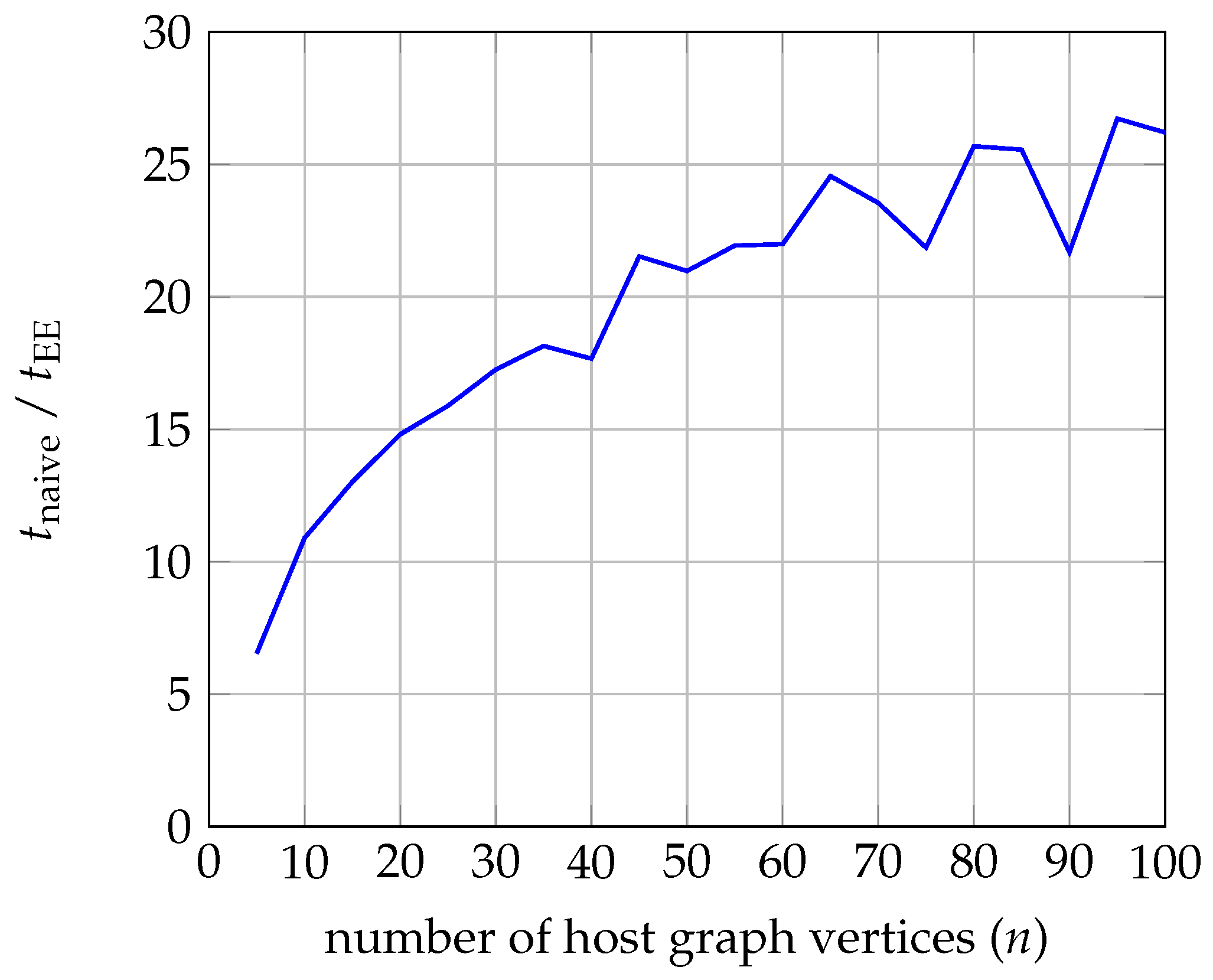
Since all three pattern graphs contain nontrivial automorphisms, the EE-aware algorithm is significantly faster in all cases. As expected, the difference is most pronounced when searching for the occurrences of the graph $K_4$. The optimal EE partition of this graph has a score of 24; the corresponding values for the graphs $L_4$ and $C_4$ are 2 and 4, respectively. Theoretically, these are the upper bounds for the ratio $t_{\mathrm{naive}}/t_{\mathrm{EE}}$. However, owing to idiosyncrasies associated with implementation, execution, and time measurements, the actual ratio may also be slightly larger.

In the case of $L_4$ and $C_4$, the actual ratios are fairly close to the upper bounds. In the case of $K_4$, the ratio tends to increase as the number of occurrences grows. This trend has been confirmed by an experiment in which we searched for the occurrences of the graph $K_4$ within the graph $K_n$ (the full graph on n vertices) for $n\in \{5,10,15,\dots ,100\}$. Figure 9 displays a plot of the ratio $t_{\mathrm{naive}}/t_{\mathrm{EE}}$ as a function of n. Note that the number of occurrences of $K_4$ in $K_n$ is $\left(\genfrac{}{}{0pt}{}{n}{4}\right)$.

9. Conclusions and Discussion

In this paper, we present a new view on graph symmetries in the form of a graph partition called exploratory equivalence. We show how such partitions can be used for symmetry breaking without imposing any other restrictions or overhead during the execution of backtracking algorithms. Since there are many possible exploratory equivalent partitions in a graph, we introduce the so-called MaxEE optimization problem, which captures the efficiency of symmetry breaking. We manage to position the verifier for the optimization problem between the graph isomorphism and set stabilizer problems. This makes the optimization problem not yet known to be in $\mathcal{NP}$. Despite this pessimistic result, we propose optimal polynomial-time algorithms for cycles and trees and a practical heuristic algorithm for general graphs.

As part of the presented results, we show that MaxEE does not capture all possible symmetries in graphs and also show examples of suboptimal results of the given heuristics. However, we also conducted a small experiment, which indicates that in practice MaxEE captures a vast majority of symmetries and also that the greedy algorithm produces optimal results in most cases.

The settings of the experiment are as follows. We generated all connected (non-isomorphic) graphs of sizes 4–10 using geng [46]. For each of them, we computed the number of automorphisms (the number of all symmetries), the optimal solution to MaxEE using backtracking search, and the solution given by the greedy heuristics.

Table 4. Empirical evaluation of MaxEE on the set of all connected simple graphs of sizes 4–10 nodes. We counted the cumulative number of all symmetries on these sets ($\mathrm{sym}.$), the sum of all optimal goal values for MaxEE ($\mathrm{opt}.$), and the sum of all goal values obtained by the greedy heuristics ($\mathrm{greedy}$).

Size	# of Graphs	sym.	opt.	$\frac{\mathbf{opt}.}{\mathbf{sym}.}$	Greedy	$\frac{\mathbf{greedy}}{\mathbf{opt}.}$
4	6	46	42	0.91	42	1.0
5	21	242	226	0.93	226	1.0
6	112	1650	1522	0.92	1490	0.97
7	853	11,338	10,910	0.96	10,850	0.99
8	11,117	100,648	96,896	0.96	96,588	0.99
9	261,080	1,154,556	1,133,514	0.98	1,131,216	0.99
10	11,716,571	24,724,920	24,529,766	0.99	24,515,292	0.99

summarizes these results. For each size (4–10), we show the cumulative number of all symmetries (sym.), the number of symmetries captured by MaxEE (opt.), and the number of symmetries captured by the greedy heuristics (greedy). We have to point out that finding the optimal solution for all graphs of size 10 took a substantial computational effort. We used 77 computers (off-the-shelf personal computers), and it took us nearly one day to obtain the results. On the other hand, the heuristic method was run on a single computer, and the results were obtained in a couple of hours. This is a simple indication of the practical feasibility of the heuristic method.

In this simple experiment, two observations can be made. The first is that, even though MaxEE does not capture all the symmetries present in graphs, it does capture a huge percentage of them (see $\frac{\mathrm{opt}.}{\mathrm{sym}.}$ column in Table 4). The second observation is the quality of the greedy algorithm, which on average produces nearly optimal results (see $\frac{\mathrm{greedy}.}{\mathrm{opt}.}$ column in Table 4). The percentage of captured symmetries increases with the size of the graphs, which also means that the optimal solution captures more than 99% (on average) of symmetries in the graphs. These results are very encouraging, demonstrating the practical feasibility of the methods presented in this paper.

From our entire work and the empirical feature of subgraph isomorphism, we can summarize the properties of our proposed method as follows:

• The approach is suitable when mapping small graphs onto large graphs, since the overhead of searching for good partitions is minimal. Such application arise often in the field of bioinformatics [47] and in many applications that use graph databases [48].
• Since it was empirically established in [49], symmetries arise surprisingly often in real graphs, which makes it a compelling argument to finally introduce a symmetry-breaking method into state-of-the-art solvers.
• As mentioned above, one of the goals to design a lightweight mechanism, which would induce a minimal overhead in the backtracking algorithm. We achieved this goal, since after the exploratory equivalent partition is detected (as part of the preprocessing), the backtracking algorithm just utilizes the induced constraints which follow from the partition.
• As a downside, the method might become unfeasible when very large graphs are being mapped. However, in such cases, other methods might also fail to find solutions in reasonable time.

In our future work, we will incorporate our equivalence into state-of-the-art solvers and conduct extensive testing on a variety of benchmark problems. This will show us the empirical usability of the presented concept and finally establish symmetry-breaking as a standard component of subgraph isomorphism solvers. Since our framework is designed for a wide variety of problems, we intend to integrate exploratory equivalence into some of these as well, e.g., largest clique problem, tree-width, etc. In the more theoretical part of our future work, we will investigate the time complexity of the MaxEE problem further and design new heuristics for finding exploratory equivalent partitions even more quickly.