Braids, 3-Manifolds, Elementary Particles: Number Theory and Symmetry in Particle Physics

Abstract

In this paper, we will describe a topological model for elementary particles based on 3-manifolds. Here, we will use Thurston’s geometrization theorem to get a simple picture: fermions as hyperbolic knot complements (a complement $C\left(K\right)=S^3\backslash (K\times D^2)$ of a knot K carrying a hyperbolic geometry) and bosons as torus bundles. In particular, hyperbolic 3-manifolds have a close connection to number theory (Bloch group, algebraic K-theory, quaternionic trace fields), which will be used in the description of fermions. Here, we choose the description of 3-manifolds by branched covers. Every 3-manifold can be described by a 3-fold branched cover of $S^3$ branched along a knot. In case of knot complements, one will obtain a 3-fold branched cover of the 3-disk $D^3$ branched along a 3-braid or 3-braids describing fermions. The whole approach will uncover new symmetries as induced by quantum and discrete groups. Using the Drinfeld–Turaev quantization, we will also construct a quantization so that quantum states correspond to knots. Particle properties like the electric charge must be expressed by topology, and we will obtain the right spectrum of possible values. Finally, we will get a connection to recent models of Furey, Stoica and Gresnigt using octonionic and quaternionic algebras with relations to 3-braids (Bilson–Thompson model).

1. Introduction

General relativity (GR) deepens our view on space-time. In parallel, the appearance of quantum field theory (QFT) gives us a different view of particles, fields and the measurement process. One approach for the unification of QFT and GR, to a quantum gravity, starts with a proposal to quantize GR and its underlying structure, space-time. Here, there is a unique opinion in the community about the relation between geometry and quantum theory: the geometry as used in GR is classical and should emerge from a quantum gravity in the usual limit that Planck’s constant tends to zero. Most theories went a step further and try to get the spacetime directly from quantum theory. As a consequence, the used model of a smooth manifold cannot be used to describe quantum gravity. However, currently, there is no real sign for a discrete spacetime structure or higher dimensions in current experiments [1]. Therefore, in this work, we conjecture that the model of spacetime as a smooth 4-manifold can be also used in the quantum gravitational regime. As a consequence, one has to find geometrical/topological representations for quantities in QFT (submanifolds for particles or fields, etc.) as well in order to quantize GR. In this paper, we will tackle this problem to get a geometrical/topological description of the standard model of elementary particle physics. Recently, there were efforts by Furey [2,3,4,5], Gresnigt [6,7,8] and Stoica [9] to use octonions and Clifford algebras to get a coherent model to describe the particle generations in the standard model. In the past, the stability of matter was related to topology like in the approach of Lord Kelvin [10] with knotted aether vortices. The proposal to derive matter from space was considered by Clifford as well by Einstein, Eddington, Schrödinger and Wheeler with only partial success (see [11,12]). Giulini [13] discussed the status of geometrodynamics in establishing particle properties like spin from spacetime by using special solutions of general relativity. The usage of knots and links to model particles, like the electron, neutrinos, etc., was firstly observed by Jehle [14]. The phenomenological description of particle properties by using the quantum group $S{U}_q\left(n\right)$ is given in the work of Gavrilik [15]. Here, the (deformation) parameter q of $S{U}_q\left(n\right)$ was linked with the flavor mixing angle (Cabibbo angle). Furthermore, torus knots as given by 2-braids were associated with vector mesons (vector quarkonia) of different flavors. Later, Finkelstein [16] used the representation of knots by quantum groups for his particle model. Similar ideas are discussed in the model of Bilson–Thompson [17] in its loop theoretic extension [18]. Even for the Bilson–Thompson model, Gresnigt found a link between Furey’s approach and this model. However, some properties of the Bilson–Thompson model remained mysterious, like the definition of the charge. Open is also the meaning of the braiding. If there is a connection between spacetime and matter, then one has to construct the known fermions and bosons directly. Here, it seems that the main problem is the determination of the underlying spacetime. In this paper, we will follow this way with an heuristic argument for the spacetime to be the K3 surface in Section 3. Then, we will analyze this spacetime by using branched covers to find two suitable substructures, a knot complement representing the fermions and a link complement to represent the bosons. Here, we profit from ideas by Duston [19,20,21] as well from the work of Denicola, Marcolli and al-Yasry [22]. As a byproduct, we also found interesting relations to octonions. The representation of the knot and link complements by branched covers gives the link to the original Bilson–Thompson model [17] but also to Gresnigt’s work [6]. In Section 5, we will discuss the electric charge and construct the corresponding operator by using the underlying $U\left(1\right)$ gauge theory by using the Hirzebruch defect. Finally, we will obtain the correct charge spectrum: fermions carry the charges $0,\pm \frac{1}{3},\pm \frac{2}{3},\pm 1$ in units of the unit charge e. Here, the factor $\frac{1}{3}$ is related to 4-dimensional topology (Hirzebruch signature theorem). In Section 6, we will discuss the independence of the particular braid from the particle. The braid is connected with the state of the particle as shown by using the Drinfeld–Turaev quantization. Finally, we finish the paper with some speculations about the number of generations, given by the number of $S^2\times S^2$ parts in the spacetime (K3 surface), and a global symmetry, the group $PGL(3,4)$ of $3\times 3$ matrices of the 4-element field $F_4$, induced from the K3 surface by using umbral moonshine.

Before we start with the description of the model, we will discuss the key arguments and scope of the model. The model is based on a smooth spacetime that is described by a smooth 4-manifold. First, it is argued that this spacetime is the K3 surface where the evolution of the cosmos is submanifold. By using this model, the calculation of cosmic parameters (cosmological constant, inflation parameters, etc.) matches with the experimental results. For the following, we use the characterization of 4-manifold (i.e., the spacetime) by surfaces that are connected to complements of links and knots (3-manifolds with boundary). Interestingly, both 3-manifolds have a meaning by our previous work: knot complements are fermions and link complements are bosons. Here, we find a representation of both 3-manifolds by braids of three strands (3-braids), which is the connection to the work of Bilson–Thompson and Gresnigt. In case of the K3 surface as spacetime, the surfaces mentioned above are arranged with a strong connection to octonions, which is the link to Furey’s work. To connect fermions, one needs a special class of link complements, so-called torus bundles, which can be interpreted as gauge fields. Interestingly, there are only three classes of torus bundles and we were able to connect them with the gauge groups $U\left(1\right),SU\left(2\right),SU\left(3\right)$. The main result of the paper is definition and interpretation of the electric charge. The electric charge is a topological invariant (Hirzebruch defect). For the fermions (knot complements), we obtained the spectrum $\{0,\pm 1,\pm 2,\pm 3\}$ which agrees with the observation (normalized in $e/3$ units). The discussion about the quantization of the model and the number of generations closes the paper.

The model uses a classical spacetime. Quantum properties are not included in an obvious way. We obtained the correct charge spectrum, but we do not know the direct connection between knot complement and fermion (electron, neutrino, quark). There are ideas to use a quantization by a change of the smoothness structure, known as Smooth Quantum Gravity [23]. In principle, the number of generations is connected with the spacetime. We got the minimal value of three generations, but it is only a lower bound. The model produces only the particles of the standard model. No supersymmetry or other extensions of the standard model can be derived by this model. Currently, we also have no idea to calculate the coupling constants and masses. It seems that these parameters are connected with the topological property of the spacetime.

2. Preliminaries: Branched Coverings of 3- and 4-Manifolds

According to Alexander (see [24] for instance), every manifold $M^n$ can be represented as p-fold branched covering $\pi :M^n\to S^n$ along an $n-2$ dimensional subcomplex $N^{n-2}\subset S^n$, the branching set. In detail, the map $\pi$ is a covering except for the branching set, i.e., for every point $b\in S^n\backslash N^{n-2}$ the map ${\pi }^{-1}\left(b\right)$ consists of p points and the neighborhood $U\left(b\right)$ is homeomorphic to one component ${\pi }^{-1}U\left(b\right)$. Then, $M^n\backslash {\pi }^{-1}\left(N^{n-2}\right)\to S^n\backslash N^{n-2}$ is a $p-$fold covering. Usually, $N^{n-2}$ has the structure of a simplicial subcomplex. The $p-$fold covering is completely determined by the representation ${\pi }_1(S^n\backslash N^{n-2})\to S_p$ in the permutation group $S_p$ of p symbols. Before going into the details, we will look at some examples. First, there are no branched coverings for 1-manifolds except for a trivial one. The first interesting example is given by a compact 2-manifold, i.e., by a surface of genus g. Here, the branching set consists of a finite number of points (0-dimensional branching set). The branching set of 3-manifolds is a one-dimensional, complex and we will later see that knots and links are the appropriated structures. In case of 4-manifolds, one has a two-dimensional complex as a branching set that was shown to be a surface. These facts are easy to understand, but one parameter of a branched covering is open: how many folds are minimally needed to represent every manifold in a fixed dimension, or, how large is p minimally for a manifold of dimension n?

2.1. As Warmup: Branched Coverings of 2-Manifolds

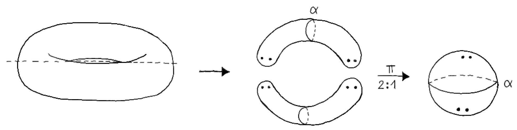
Let us start with the simplest case, the surface. By results of Riemann and Hurwitz, every surface can be represented by a 2-fold covering of $S^2$. As example, let us take the torus $T^2$ with the 2-fold covering $T^2\to S^2$ branched along four points. The idea of the construction is simple: choose a symmetry axis so that the genus g surface can be generated by a rotation (see Figure 1).

This axis meets the surface in 4g points which are the branching points of the covering.

2.2. Branched Coverings of 3-Manifolds

For a 3-manifold, one has a one-dimensional, branching set and a result of Alexander states that this branching set is a link with a finite number of components. Later, Hirsch, Hilden and Montesinos [25,26,27] obtained independently the result that every closed, compact 3-manifold can be represented as a 3-fold branched covering of the 3-sphere branched along a knot. As an example, consider the Poincare sphere $\mathsf{\Sigma }(2,3,5)$ that can be represented by a 3-fold covering $\mathsf{\Sigma }(2,3,5)\to S^3$ branched along the $(2,5)$ or $(5,2)$ torus knot. Now, let us consider a closed, compact 3-manifold $N^3$ with a 3-fold branched covering $N^3\to S^3$ branched along a knot K. It means that the map $N^3\backslash K\to S^3\backslash K$ is a real $3:1$ map. Interestingly, there is a diffeomorphism between $N^3\backslash K$ and $S^3\backslash K$ so that the $3:1$ covering map is now given by $S^3\backslash K\to S^3\backslash K$. Furthermore, the 3-fold covering is completely determined by the map ${\pi }_1(S^3\backslash K)\to S_3$, the representation of the fundamental group into the permutation group $S_3$ of three letters. A simple extension of the $S_3$ by considering the order of the permutations gives the braid group $B_3$ of three strands. In principle, the minimal number of folds $p=3$ is the root for the description of particles by 3-braids, as shown later on.

2.3. Branched Covering of 4-Manifolds

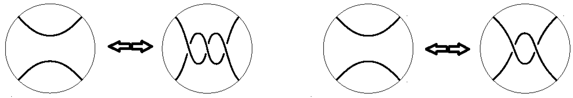
In a similar manner, one would expect that every 4-manifold $M^4$ can be represented as 4-fold branched covering of $S^4$ branched along a surface. Piergallini [28] was able to show something similar, but the surface is only immersed and admits a finite number of singularities (cusps and nodes). If one adds an additional sheet, getting a 5-fold branched covering, then one can omit these singularities (thus getting a locally flat embedded surface) [29]. For a better understanding, we will discuss the way to this result shortly. In [28], Piergallini considered the possible transformations or changes of the branching set for a 3-manifold $N^3$, i.e., the knot. Amazingly, he found two possible changes (see Figure 2).

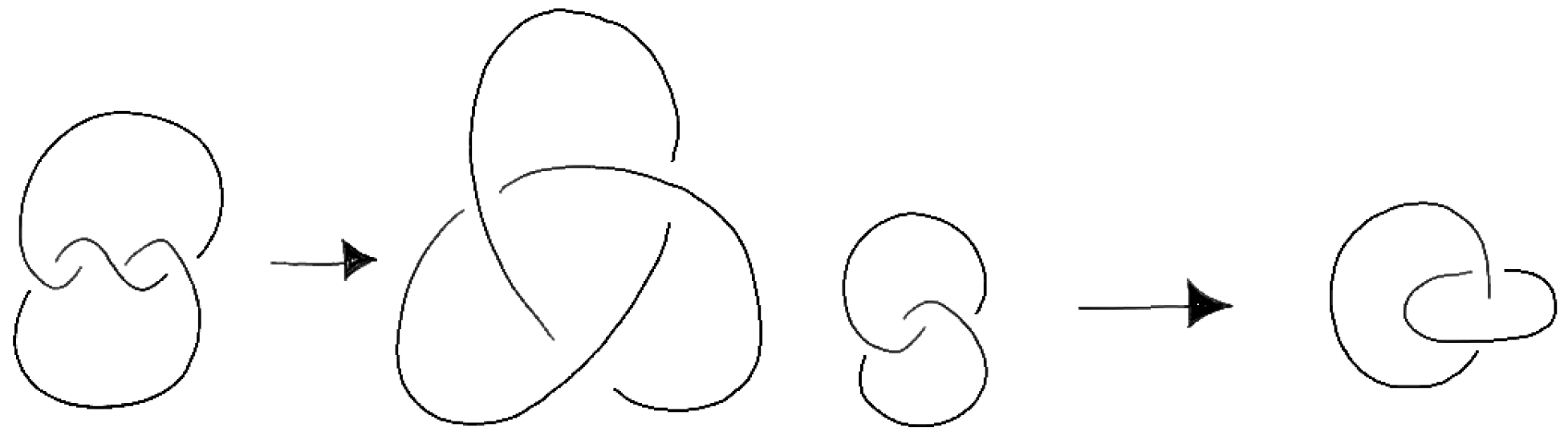
All changes do not affect the underlying 3-manifold $N^3$, i.e., he found different knots and links representing the same 3-manifold as a 3-fold branched cover. Then, he used this result to find a branched covering for a 4-manifold. For that purpose, he introduced the concept of an additional leaf or fold in the covering, i.e., if a 3-manifold $N^3$ is represented by a 3-fold covering, then it is also represented by a 4-fold covering. Then, he extended this 4-fold covering of $N^3$ to a 4-fold covering of $N^3\times [0,1]$ (i.e., a trivial cobordism). At the same time, the knot $K_1$ as branching set of $N^3$at one side of $N^3\times [0,1]$ (i.e., $N^3\times \left\{0\right\}$) is related to the changed knot $K_2$ as branching set of $N^3$ on the other side of $N^3\times [0,1]$ (i.e., $N^3\times \left\{1\right\}$). For the covering of $N^3\times [0,1]$, one will get a surface with two boundaries, the disjoint union $K_1\bigsqcup K_2$ of the two branching knots. This procedure can be done for the two possible changes [30]. For the first change, Piergallini got the trefoil knot at the boundary, whereas, for the second case, he obtained the Hopf link (see the Figure 3).

In dimension 4, one will get the cone over the trefoil, also known as cusp, and the cone over the Hopf link, also known as node, as singularities of the surface as a branching set of the 4-manifold. Expressed differently, the trefoil knot is the link of the cusp singularity ${\displaystyle z^2+w^3}$; the Hopf link (oriented correctly) is the link of the node singularity ${\displaystyle z^2+w^2}$. As explained in the previous subsection, we have to consider the two fundamental groups $G_P={\pi }_1(S^3\backslash \left\{trefoil\right\})$ and $G_{WW}={\pi }_1(S^3\backslash \left\{Hopf\right\})$ for the corresponding branched cover. Both groups are known and can be simply calculated to be

$$G_P=\langle a,b|aba=bab\rangle =B_3{G}_{WW}=\langle a,b,c|a{b}^{-1}{a}^{-1}b\rangle =\mathbb{Z}\oplus \mathbb{Z},$$

(1)

which is a surprising result. From the point of 4-manifolds we will get two possible 3-manifolds as boundary of the singularities: a 3-manifold (knot complement) with one boundary and a 3-manifold (link complement) with two boundaries. These two 3-manifolds can be simply interpreted: the knot complement has one boundary component and can be seen as a fermion (see also [31]) and the link complement has two boundary components and can be interpreted as interaction (see also [32]).

2.4. Branched Coverings of Knot Complements

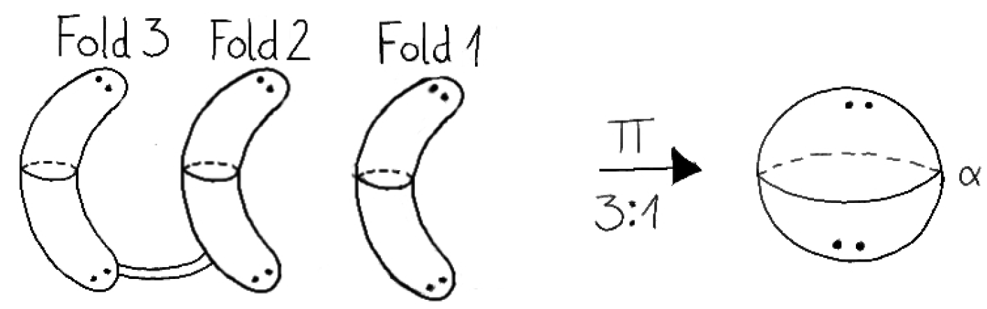
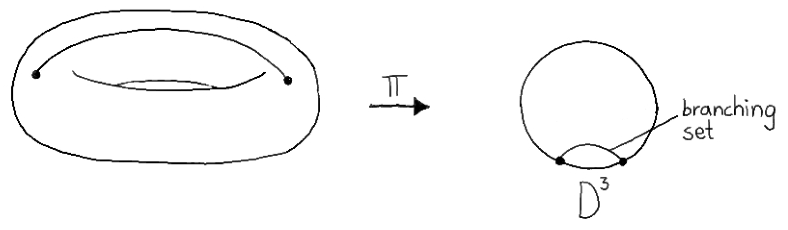
Now, we will describe the case of a 3-manifold (the knot complement) with boundary a torus $T^2$. First, we will change the 2-fold covering of the torus to a 3-fold covering by adding a trivial sheet. For that purpose, we consider the 2-fold branched covering $T^2\to S^2$ and add a 2-sphere $T^2\#S^2\to S^2\#S^2$ which changes nothing ($S\#S^2$ is diffeomorphic to S for every surface S). However, at the same time, we will obtain a 3-fold covering (see Figure 4).

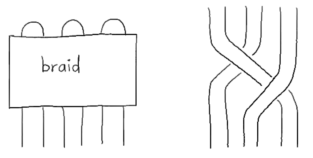
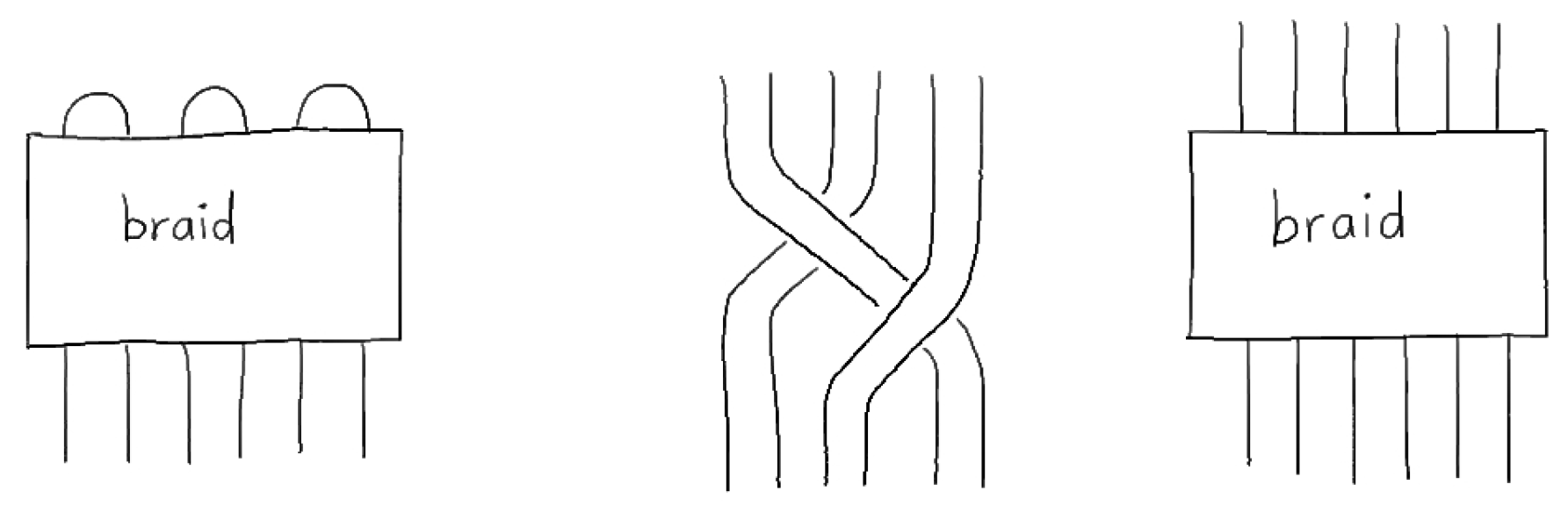
For a 3-manifold $\mathsf{\Sigma }$ with boundary $T^2$, one has to consider a branched covering $\mathsf{\Sigma }\to S^3\backslash D^3$(3-sphere with one puncture or p punctures for p boundary components). For the construction of the covering, one needs another representation of a 3-manifold, the Heegard decomposition. There, one considers two handle bodies $H_g,H_g^{\prime }$ of genus g, i.e., the sum of g copies of the solid torus $D^2\times S^1$. The gluing $H_g{\cup }_{\varphi }{H}_g^{\prime }$ of these handle bodies along the boundary using a diffeomorphism $\varphi :\partial H_g\to \partial H_g^{\prime }$(to be precise: $\varphi$ is an element of the mapping class group) produces every compact, closed 3-manifold. For the 3-sphere, one obtains a decomposition $H_1\cup H_1^{\prime }$ using two solid tori where the meridian of $H_1$ is mapped to the longitude of $H_1^{\prime }$ and vice versa. $H_g$ can be obtained by a branched covering $H_g\to D^3$ with a branching set $g+2$ arcs (see Figure 5).

The diffeomorphism $\varphi$ is represented by a braid connecting the two handle bodies where the braid closes above and below to get a link. In case of a 3-manifold with a boundary, the braid closes only on one side and we obtain a braid again (or, more generally, a tangle), see Figure 6.

The underlying braid must be also a 3-braid but represented as a 6-braid.

3. Reconstructing a Spacetime: The K3 Surface and Particle Physics

After so many years of experimental research, the standard model of particle physics and of cosmology as well general relativity are confirmed with high precision. There is no real contradicting result which shows the necessity to introduce new physics. An exception may be cosmology with the unknown components of dark matter and dark energy. However, this situation is by no means satisfying. Both standard models have a bunch of free parameters (19 parameters in particle physics, for instance). If there is no sign for new physics, how did we get these parameters? Here, we will argue that these parameters can be determined by topology. However, at first glance, this idea seems hopeless. There are infinitely many suitable topologies for the spacetime, seen as 4-manifold, and, for the space, seen as 3-manifold. Here, we will go a different way. Why not try to determine the space $\mathcal{M}$ of all possible spacetime-events? Thus, let me start with a definition: let $\mathcal{M}$ be the space of all possible spacetime events, i.e., the set of all spacetime events carrying a manifold structure. In principle, $\mathcal{M}$ can be identified with the spacetime. Then, a specific physical situation is an embedding of a 3-manifold into $\mathcal{M}$, a dynamics is an embedding of a cobordism between 3-manifolds into $\mathcal{M}$. Here, we assume implicitly that everything can be geometrically/topologically expressed as submanifolds (see [31,32]). In the following, we will try to discuss this approach and how far one can go. Some heuristic arguments are rather obvious:

• $\mathcal{M}$ is a smooth 4-manifold,
• any sequence of spacetime event has to converge to a spacetime event and
• any loop (time-like or not) must be contracted.

A dynamics is a mapping of a spacetime event to a new spacetime event. It is usually smooth (differential equations), motivating the first argument. The second argument expresses the fact that any initial spacetime event must converge to a final spacetime event, or the limit of any sequence of spacetime events must converge to a spacetime event. Then, $\mathcal{M}$ is a compact, smooth 4-manifold. The usual spacetime is an open subset of $\mathcal{M}$. The third argument above is motivated to neglect time-like loops. The spacetime is an open subset of $\mathcal{M}$ or the spacetime is embedded in $\mathcal{M}$. Now, consider a loop in the spacetime. By changing the embedding via diffeomorphisms (this procedure is called isotopy), every loop is contractable. Therefore, this argument implies that there is no time-like loops (implying causality). Finally, $\mathcal{M}$ is a compact, simply connected, smooth 4-manifold.

Now, we will restrict $\mathcal{M}$ in a manner so that we are able to determine it. For the following, we implicitly assume that the equations of general relativity are valid without any restrictions. Then, the vacuum equations are equivalent to

$$R_{\mu \nu }=0,$$

demanding Ricci-flatness. However, as shown in [33,34] and in recent years in [23,31,32], the coupling to matter can be described by a change of the smoothness structure. Therefore, the modification of the smoothness structure will produce matter (or sources of gravity). However, at the same time, we need a smoothness structure that can be interpreted as a vacuum given by a Ricci-flat metric. Therefore, we will demand that

• $\mathcal{M}$ has to admit a smoothness structure with Ricci-flat metric representing the vacuum.

Interestingly, these four demands are restrictive enough to determine the topology of $\mathcal{M}$. With the help of Yau’s seminal work [35], we will obtain that $\mathcal{M}$ is homeomorphic to the K3 surface, using Yaus’s work that there is only one compact, simply connected Ricci-flat 4-manifold. However, it is known by the work of LeBrun [36] that there are non-Ricci-flat smoothness structures. In the next step, we will determine the smoothness structure of $\mathcal{M}$. For that purpose, we will present some deep results in differential topology of 4-manifolds:

• there is a compact, contactable submanifold $A\subset \mathcal{M}$ (called Akbulut cork) so that cutting out Aand reglue it (by an involution) will produce a new smoothness structure,
• $\mathcal{M}$ splits topologically into

  $$|E_8\oplus E_8|\#\underset{3\left(S^2\times S^2\right)}{\underbrace{\left(S^2\times S^2\right)\#\left(S^2\times S^2\right)\#\left(S^2\times S^2\right)}}=2\left|E_8\right|\#3(S^2\times S^2)$$

  (2)

  two copies of the $E_8$ manifold and three copies of $S^2\times S^2$ and
• the 3-sphere $S^3$ is a submanifold of A.

In [37], we already discussed this case. Interestingly, there is always a topological 4-manifold for all combinations of $E_8$ and $S^2\times S^2$, but not all topological 4-manifolds are smooth manifolds. Let us consider the 4-manifold that splits topologically into p copies of the $|E_8|$ manifold and q copies of $S^2\times S^2$ or

$$p|E_8|\#q\left(S^2\times S^2\right).$$

Then, this 4-manifold is smoothable for every q but $p=0$ and the first combination for $p\ne 0$ is the pair of numbers $p=2,q=3$ (which is the K3 surface). Any other combination ($p=2,q<3$ or every q and $p=1$) is forbidden as shown by Donaldson [38].

Now, we consider the smooth K3 surface that is Ricci-flat, simply connected, smooth. The main part in the following discussion will be the use of the smoothness condition. As discussed above, the smoothness structure is determined by the Akbulut cork A. Furthermore, as argued above, the smoothness structure is strongly related to the appearance of matter and this process is strongly connected to the evolution of our cosmos. It is known as reheating after the inflationary phase. Therefore, the Akbulut cork (including its embedding) should represent the inflationary phase with reheating.

The Akbulut cork is built from a homology 3-sphere that will become the boundary $\partial A$. The difference to a usual 3-sphere $S^3$ is given by the so-called fundamental group, the equivalence class of closed loops up to deformation (homotopy) with concatenation as group operation. In principle, one constructs a cobordism between $S^3$ and the homology 3-sphere $\partial A$. All elements of the fundamental group will be killed by adding appropriate disks. At the end, one can add a 4-disk to get the full contractable cork A. After this short discussion, we are able to identify the first topological transition: if the cosmos starts as small 3-sphere (conjectural of Planck size), then the space changes to $\partial A$, or

$$S^3\to \partial A.$$

The topology of $\partial A$ depends strongly on the topology of $\mathcal{M}$. In case of the K3 surface, $\partial A$ is known to be a Brieskorn spheres, precisely the 3-manifold

$$\mathsf{\Sigma }(2,5,7)=\left\{x,y,z\in \mathbb{C}|x^2+y^5+z^7={0\left|x\right|}^2+{\left|y\right|}^2+{\left|z\right|}^2=1\right\}.$$

The embedding of the Akbulut cork is essential for the following results. In [39], it was shown that the embedded cork admits a hyperbolic geometry if the underlying K3 surface has an exotic smoothness structure. This simple property has far-reaching consequences. Hyperbolic manifolds of dimension three or higher are rigid, i.e., geometric properties like volume or curvature are topological invariants (Mostow-Prasad rigidity). If we assume that the cork A represents the cosmic evolution, then geometric properties like the curvature of $\partial A$ or the change of the size after the transition $S^3\to \partial A$ are connected with topological properties of the embedded cork A and of the underlying K3 surface by using Mostow–Prasad rigidity. This simple idea opens the door to explicit calculations. In case of the transition $S^3\to \partial A=\mathsf{\Sigma }(2,5,7)$, the corresponding results can be found in [39]. If one assumes a Planck-size $\left(L_P\right)$ 3-sphere at the Big Bang, then the scale a of $\mathsf{\Sigma }(2,5,7)$ changes like

$$a=L_P·exp\left(\frac{3}{2·CS\left(\mathsf{\Sigma }\right(2,5,7\left)\right)}\right)$$

with the Chern–Simons invariant

$$CS\left(\mathsf{\Sigma }(2,5,7)\right)=\frac{9}{4·(2·5·7)}=\frac{9}{280}$$

and the Planck scale of order ${10}^{-34}m$ changes to ${10}^{-15}m$. Obviously, this transition has an exponential or inflationary behavior. Surprisingly, the number of e-folds can be explicitly calculated (see [40]) to be

$$N=\frac{3}{2·CS\left(\mathsf{\Sigma }\right(2,5,7\left)\right)}+ln\left(8{\pi }^2\right)\approx 51,$$

(3)

and we also obtain the energy and time scale of this transition (see [40,41])

$$E_{GUT}=\frac{E_P}{1+N+\frac{N^2}{2}+\frac{N^3}{6}}\approx {10}^{15}GeV t=t_P\left(1+N+\frac{N^2}{2}+\frac{N^3}{6}\right)\approx {10}^{-39}s$$

(4)

right at the conjectured scale of the Grand Unified Theory (GUT) ($E_P,t_P$ Planck energy and time, respectively). In our recent work [41], this transition was analyzed in a detailed manner. There, it was shown that the transition can be described by a scalar field model which conformally agrees (as shown in [42]) with the Starobinsky-$R^2$ theory [43]. However, then, the dimension-less free parameter $\alpha ·M_P^{-2}$ as well as spectral tilt ${\displaystyle n_s}$ and the tensor-scalar ratio r can be determined to be

$$\alpha ·M_P^{-2}=1+N+\frac{N^2}{2}+\frac{N^3}{6}\approx {10}^{-5},n_s\approx 0.961r\approx 0.0046,$$

using Equation (3), which is in good agreement with current measurements. The embedding of the cork A is based on the topological structure of the K3 surface $\mathcal{M}$. As discussed above, $\mathcal{M}$ splits topologically into a 4-manifold $|E_8\oplus E_8|$ and the sum of three copies of $S^2\times S^2$ (see [44]). In the topological splitting (2), the 4-manifold $|E_8\oplus E_8|$ has a boundary that is the sum of two Poincaré spheres $P\#P$. Here, we used the fact that a smooth 4-manifold of type $|E_8|$ must have a boundary (which is the Poincaré sphere P); otherwise, it would contradict the Donaldson’s theorem [38]. Then, any closed version of $|E_8\oplus E_8|$ does not exist and this fact is the reason for the existence of an exotic ${\mathbb{R}}^4$. To express it differently, the neighborhood of the embedded cork lies between the 3-manifold $\mathsf{\Sigma }(2,5,7)$ (boundary of the cork) and the sum of two Poincaré spheres $P\#P$. Therefore, we have two topological transitions resulting from the embedding

$$S^3\stackrel{cork}{⟶}\mathsf{\Sigma }(2,5,7)\stackrel{gluing}{⟶}P\#P.$$

(5)

The transition $\mathsf{\Sigma }(2,5,7)\to P\#P$ has a different character as discussed in [39]. A direct consequence is the appearance of a cosmological constant as a direct consequence of the topological invariance of the curvature of a hyperbolic manifold. With respect to the critical density, the final formula for normalized cosmological constant, denoted by ${\mathsf{\Omega }}_{\mathsf{\Lambda }}$, reads

$${\mathsf{\Omega }}_{\mathsf{\Lambda }}=\frac{c^5}{24{\pi }^{2}hG{H}_0^2}·exp\left(-\frac{3}{CS\left(\mathsf{\Sigma }\right(2,5,7\left)\right)}-\frac{3}{CS(P\#P)}-\frac{\chi \left(A\right)}{4}\right).$$

The Chern–Simons invariants $CS(P\#P)=\frac{1}{60},CS\left(\mathsf{\Sigma }(2,5,7)\right)=\frac{9}{280}$ and the Euler characteristics of the cork $\chi \left(A\right)=1$ together with the Hubble constant (see [45,46] combined with [47])

$${\left(H_0\right)}_{Planck+Hubble}=69,2\frac{km}{s·Mpc}$$

gives the value

$${\mathsf{\Omega }}_{\mathsf{\Lambda }}\approx 0.7029,$$

which is in excellent agreement with the measurements. The numerical results above illustrate the power of the main idea to use topology to fit the parameter in the standard model of cosmology. Interestingly, these parameters are also important for particle physics. The existence of two transitions (5) implies in the formalism above the existence of two different energy scales, the GUT scale of the first transition and a scale of Higgs mass order $126GeV$ for the second transition. These two scales are the right input for the see-saw mechanism to generate a tiny neutrino mass (see [40]). Secondly, the formalism also provides a favor regarding the existence of a right-handed neutrino. The energy scale of the two transitions $S^3\to \mathsf{\Sigma }(2,5,7)\to P\#P$ can be expressed as a mass (via $M{c}^2$), and we obtain

$$M=\sqrt{\frac{4\hslash c}{G}}\left(\frac{exp\left(-\frac{1}{2·CS(P\#P)}\right)}{1+N+\frac{N^2}{2}+\frac{N^3}{6}}\right)\approx 126.4GeV,$$

(6)

which agrees with the mass of the Higgs boson (see [40]). Then, the Higgs boson can be expressed as the result of a topological transition (see [48]). Now, we will use the two energy scales to generate the neutrino mass. For that purpose, we start with the non-diagonal mass matrix

$$\left(\begin{array}{cc}0& M\\ M& B\end{array}\right)$$

with two mass scales B and M fulfilling $M\ll B$. This matrix has eigenvalues

$${\lambda }_1\approx B{\lambda }_2\approx -\frac{M^2}{B}$$

so that ${\lambda }_1$ is the mass of the right-handed neutrino, and ${\lambda }_2$ represents the mass of the left-handed neutrino. Now, we will use the two scales (4) and (6)

$$B\approx 0.67·{10}^{15}GeV,M\approx 126.4GeV,$$

and we will obtain for the neutrino mass

$$m=\frac{M^2}{B}\approx 0.024eV,$$

which is in good agreement with the constraints from the PLANCK mission.

These results seem to support our view that the K3 surface can be the underlying spacetime (as seen as the set of all possible spacetime events). The evolution of the cosmos is a suitable subset of this space.

4. From K3 Surfaces to Octonions, 3-Braids and Particles

The results of the previous section illustrated the power of the approach and its relation to particle physics. In this section, we will discuss the topological reasons and the relation to the models of Furey, Gresnigt and Bilson–Thompson. In these models, 3-braids, octonions and quaternions play a key role. Therefore, we have to understand how these structures will naturally appear in the K3 surface.

4.1. K3 Surfaces and Octonions

The starting point for the description of any K3 surface is the topological splitting (2)

$$2|E_8|\#3(S^2\times S^2).$$

The K3 surface is a closed, compact, simply connected 4-manifold. According to Freedman [49], the topology is uniquely given by the intersection form, a quadratic form on the second homology characterizing the intersections of the generators as given by surfaces. The K3 surface has the intersection form

$$Q_{K3}=E_8\oplus E_8\oplus \left({\oplus }_3\left(\begin{array}{cc}0& 1\\ 1& 0\end{array}\right)\right):=2E_8\oplus 3H,$$

(7)

with the the matrix $E_8$:

$$E_8=\left[\begin{array}{cccccccc}2& 1& 0& 0& 0& 0& 0& 0\\ 1& 2& 1& 0& 0& 0& 0& 0\\ 0& 1& 2& 1& 0& 0& 0& 0\\ 0& 0& 1& 2& 1& 0& 0& 0\\ 0& 0& 0& 1& 2& 1& 0& 1\\ 0& 0& 0& 0& 1& 2& 1& 0\\ 0& 0& 0& 0& 0& 1& 2& 0\\ 0& 0& 0& 0& 1& 0& 0& 2\end{array}\right].$$

(8)

This matrix is also the Cartan matrix of the Lie algebra $E_8$ and here is where the connection to the octonions starts. For this purpose, we have to deal with the root system of the Lie algebra $E_8$. Consider a semi-simple Lie algebra G and its Cartan subalgebra $H=(H_1,\dots ,H_r)$, where r is the rank of G. This subalgebra is usually considered in the Cartan basis with the non-Hermitian generators $E_k$ and their conjugates $E_{-k}$. $E_k$ is associated with the root vector $r_m^{\left(k\right)}$ such that

$$[H_m,E_{\pm k}]=\pm r_m^{\left(k\right)}{E}_{\pm m}.$$

When the rank r is 1; 2; 4 or 8, we can combine the operators $H_m$ and the vectors $r_m^{\left(k\right)}$ (or eigenvalues) into elements of a division algebra with imaginary units $e_i$:

$$H=H_0+e_i{H}_i{r}^{\left(k\right)}=r_0^{\left(k\right)}+e_i{r}_i^{\left(k\right)}$$

so that

$$[H,E_{\pm k}]=\pm r^{\left(k\right)}{E}_{\pm k}.$$

For the Lie algebras of the groups $SU\left(2\right),O\left(4\right),O\left(8\right)$, one can construct the real numbers $\mathbb{R}$, the complex numbers $\mathbb{C}$ and the quaternions $\mathbb{H}$, respectively. Interestingly, the triality of the $O\left(8\right)$ group reflects the symmetry of the three quaternionic units $e_i=-i{\sigma }_i$, where ${\sigma }_i$ are the Pauli matrices. The case of $E_8$ was worked out by Coxeter [50] in connection with 8-dimensional regular solids and corresponds to the octonions $\mathbb{O}$. There are 240 rational points on the unit sphere $S^7$ represented by integer octonions that correspond to the 240 roots of $E_8$. We first introduce octonionic imaginary units $e_{\alpha }$$(\alpha =1,\dots ,7)$ with the multiplication rule

$$e_{\alpha }{e}_{\beta }=-{\delta }_{\alpha \beta }+{\psi }_{\alpha \beta \gamma }{e}_{\gamma },$$

with ${\psi }_{\alpha \beta \gamma }$ as a third rank antisymmetric tensor that is non-zero and equal to one for the index triples $123,246,435,367,651,572,714$. Now, we define the special element

$$h=\frac{1}{2}\left(e_1+e_2+e_3+e_7\right).$$

Then, $1;e_7;e_2;e_6,$ together with $h;eh;e_{2}h;e_{7}h$ correspond to one possible set of principal positive roots. These elements are also forming the Dynkin diagram of the root system of the $E_8$. The matrix $E_8$ in Equation (8) above is the Cartan matrix with entry $(i,j)$ defined by

$$2\frac{\langle r_i,r_j\rangle }{\langle r_i,r_i\rangle }$$

the scalar products between the root vectors $r_i$. Then, the whole approach showed that simple combinations of the octonionic imaginary units are corresponding to generators of the second homology groups for a 4-manifold having the matrix $E_8$ as an intersection form. In case of the K3 surface, one has the intersection form containing the matrix $E_8\oplus E_8$ which corresponds to two copies of octonions $\mathbb{O}\times \mathbb{O}$. Here, there is a link to the recent work [8] of complex sedions. Now, every element of $\mathbb{O}$ is related to a surface (unique up to homotopy). In the next section, we will present a connection of these surfaces to spinors.

4.2. From Immersed Surfaces in K3 Surfaces to Fermions and Knot Complements

In the previous subsection, we described a relation between the octonions and a system of eight intersecting surfaces in the K3 surface. In this system of surfaces, every surface has two self-intersections (the diagonal of the matrix (8)). Therefore, every surface is not embedded but immersed in the K3 surface. For immersed surfaces, there is a whole theory, called Weierstrass representation, with a close connection between immersed surfaces and spinors. The following discussion is borrowed from [32], and we will present it here again for completeness. First, we start with the immersion $I:\mathsf{\Sigma }\to {\mathbb{R}}^3$ of a surface $\mathsf{\Sigma }$ into ${\mathbb{R}}^3$. This immersion I can be defined by a spinor $\phi$ on $\mathsf{\Sigma }$ fulfilling the Dirac equation

$$D\phi =H\phi ,$$

(9)

with ${\left|\phi \right|}^2=1$ (or an arbitrary constant) (see Theorem 1 of [51]). A spinor bundle over a surface splits into two sub-bundles $S=S^{+}\oplus S^{-}$, representing spinors of different helicity, with the corresponding splitting of the spinor $\phi$ in components

$$\phi =\left(\begin{array}{c}{\phi }^{+}\\ {\phi }^{-}\end{array}\right),$$

and we have the Dirac equation

$$D\phi =\left(\begin{array}{cc}0& {\partial }_z\\ {\partial }_{\overline{z}}& 0\end{array}\right)\left(\begin{array}{c}{\phi }^{+}\\ {\phi }^{-}\end{array}\right)=H\left(\begin{array}{c}{\phi }^{+}\\ {\phi }^{-}\end{array}\right)$$

with respect to the coordinates $(z,\overline{z})$ on $\mathsf{\Sigma }$. In dimension 3, the spinor bundle has the same fiber dimension as the spinor bundle S (but without a splitting $S=S^{+}\oplus S^{-}$into two sub-bundles). Now, we define the extended spinor $\varphi$ over the 3-torus $\mathsf{\Sigma }\times [0,1]$ via the restriction ${\varphi |}_{T^2}=\phi$. The spinor $\varphi$ is constant along the normal vector ${\partial }_N\varphi =0$ fulfilling the three-dimensional Dirac equation

$$D^{3D}\varphi =\left(\begin{array}{cc}{\partial }_N& {\partial }_z\\ {\partial }_{\overline{z}}& -{\partial }_N\end{array}\right)\varphi =H\varphi$$

(10)

induced from the Dirac equation (9) via restriction and where ${\left|\varphi \right|}^2=const.$ In this picture, we shift the description from surfaces to 3-manifolds. The description above showed that the essential information is contained in the surface, but fermions are at least three-dimensional objects: fermions and bosons appear beginning with dimension 3 (irreducible representation of the group $SO\left(3\right)$ as given by the lift to $SU\left(2\right)$). In dimension 2, we have anyons with a spin of any rational number. However, how did we get the corresponding 3-manifold representing the fermion?

To answer this question, we consider the branched covering of the K3 surface M. As explained above, it must be a 4-fold covering $M\to S^4$ branched along a surface with singularities of two types cusp and fold. The cusp can be described as a cone over the trefoil knot, whereas the fold is the cone over the Hopf link (see Figure 9 in [30]). Now, we consider a 4-manifold with boundary, for instance by cutting out a 4-disk $D^4$ form M to get 4-manifold $M\backslash D^4$ with boundary $\partial (M\backslash D^4)=S^3$, the 3-sphere. Then, the branched covering of M induced a branched covering of the boundary $\partial M$, so that the branching set of M, a surface, induces a branching set of $\partial M$, a knot or link. In our case, the singularities of the surface (cusp and fold) given as cones over the trefoil knot and Hopf link will correspond to the trefoil knot and Hopf link in the 3-sphere. Then, the branched covering is given by the mappings of the complements $S^3\backslash \left\{trefoil\right\}$ and $S^3\backslash \left\{Hopf-link\right\}$ to the permutation group $S_3$. We see the appearance of these two complements as a sign to use these structures as particles and interactions. The complement of the knot is a 3-manifold with one boundary component. In contrast, the complement of the link looks like a cylinder $T^2\times [0,1]$ which can connect two knot complements. Therefore, we have the conjecture that knot complements are fermions and link complements are bosons.

4.3. Fermions as Knot Complements

In this section, we will discuss the topological reasons for the identification of knot complements with fermions. In our paper [31], we obtained a relation between an embedded 3-manifold and a spinor in the spacetime. The main idea can be simply described by the following line of argumentation. Let $\iota :\mathsf{\Sigma }\hookrightarrow M$ be an embedding of the 3-manifold $\mathsf{\Sigma }$ into the 4-manifold M with the normal vector $\overrightarrow{N}$ so that a small neighborhood $U_{ϵ}$ of $\iota \left(\mathsf{\Sigma }\right)\subset M$ looks like $U_{ϵ}=\iota \left(\mathsf{\Sigma }\right)\times [0,ϵ]$. Every 3-manifold admits a spin structure with a spin bundle, i.e., a principal $Spin\left(3\right)=SU\left(2\right)$ bundle (spin bundle) as a lift of the frame bundle (principal $SO\left(3\right)$ bundle associated with the tangent bundle). Furthermore, there is a (complex) vector bundle associated with the spin bundle (by a representation of the spin group), called spinor bundle $S_{\mathsf{\Sigma }}$. Now, we meet the usual definition in physics: a section in the spinor bundle is called a spinor field (or a spinor). In general, the unitary representation of the spin group in D dimensions is $2^{[D/2]}$-dimensional. From the representational point of view, a spinor in four dimensions is a pair of spinors in dimension 3. Therefore, the spinor bundle $S_M$ of the 4-manifold splits into two sub-bundles $S_M^{\pm }$ where one sub-bundle, say $S_M^{+},$ can be related to the spinor bundle $S_{\mathsf{\Sigma }}$ of the 3-manifold. Then, the spinor bundles are related by $S_{\mathsf{\Sigma }}={\iota }^{*}{S}_M^{+}$ with the same relation $\varphi ={\iota }_{*}\mathsf{\Phi }$ for the spinors ($\varphi \in \mathsf{\Gamma }\left(S_{\mathsf{\Sigma }}\right)$ and $\mathsf{\Phi }\in \mathsf{\Gamma }\left(S_M^{+}\right)$). Let ${\nabla }_X^M,{\nabla }_X^{\mathsf{\Sigma }}$ be the covariant derivatives in the spinor bundles along a vector field X as section of the bundle $T\mathsf{\Sigma }$. Then, we have the formula

$${\nabla }_X^M\left(\mathsf{\Phi }\right)={\nabla }_X^{\mathsf{\Sigma }}\varphi -\frac{1}{2}\left({\nabla }_X\overrightarrow{N}\right)·\overrightarrow{N}·\varphi$$

(11)

with the embedding $\varphi \mapsto \left(\begin{array}{c}0\\ \varphi \end{array}\right)=\mathsf{\Phi }$ of the spinor spaces from the relation $\varphi ={\iota }_{*}\mathsf{\Phi }$. Here, we remark that, of course, there are two possible embeddings. For later use, we will use the left-handed version. The expression ${\nabla }_X\overrightarrow{N}$ is the second fundamental form of the embedding where the trace $tr\left({\nabla }_X\overrightarrow{N}\right)=2H$ is related to the mean curvature H. Then, from (11), one obtains the following relation between the corresponding Dirac operators

$$D^M\mathsf{\Phi }=D^{\mathsf{\Sigma }}\varphi -H\varphi$$

(12)

with the Dirac operator $D^{\mathsf{\Sigma }}$ on the 3-manifold $\mathsf{\Sigma }$. In [32], we extend the spinor representation of an immersed surface into the 3-space to the immersion of a 3-manifold into a 4-manifold according to the work in [51]. Then, the spinor $\varphi$ defines directly the embedding (via an integral representation) of the 3-manifold. Then, the restricted spinor ${\mathsf{\Phi }|}_{\mathsf{\Sigma }}=\varphi$ is parallel transported along the normal vector and $\mathsf{\Phi }$ is constant along the normal direction (reflecting the product structure of $U_{ϵ}$). However, then the spinor $\mathsf{\Phi }$ has to fulfill

$$D^M\mathsf{\Phi }=0$$

(13)

in $U_{ϵ}$ i.e., $\mathsf{\Phi }$ is a parallel spinor. Finally, we get

$$D^{\mathsf{\Sigma }}\varphi =H\varphi$$

(14)

with the extra condition ${\left|\varphi \right|}^2=const.$ (see [51] for the explicit construction of the spinor with ${\left|\varphi \right|}^2=const.$ from the restriction of $\mathsf{\Phi }$). The idea of the paper [31] was the usage of the Einstein–Hilbert action for a spacetime with boundary $\mathsf{\Sigma }$. The boundary term is the integral of the mean curvature for the boundary; see [52,53]. Then by the relation (14) we will obtain

$$\underset{\mathsf{\Sigma }}{\int }H\sqrt{h}{d}^{3}x=\underset{\mathsf{\Sigma }}{\int }\overline{\varphi }{D}^{\mathsf{\Sigma }}\varphi \sqrt{h}{d}^{3}x$$

(15)

using ${\left|\varphi \right|}^2=const.$ As shown in [31], the extension of the spinor $\varphi$ to the 4-dimensional spinor $\mathsf{\Phi }$ by using the embedding

$$\mathsf{\Phi }=\left(\begin{array}{c}0\\ \varphi \end{array}\right)$$

(16)

can be only seen as embedding, if (and only if) the 4-dimensional Dirac equation

$$D^M\mathsf{\Phi }=0$$

(17)

on M is fulfilled (using relation (12)). This Dirac equation is obtained by varying the action

$$\delta \underset{M}{\int }\overline{\mathsf{\Phi }}{D}^M\mathsf{\Phi }\sqrt{g}{d}^{4}x=0.$$

(18)

In [31], we went a step further and discussed the topology of the 3-manifold leading to a fermion. On general grounds, one can show that a fermion is given by a knot complement admitting a hyperbolic structure. However, for hyperbolic manifolds (of dimension greater than 2), one has the important property of Mostow rigidity where geometric expressions like the volume are topological invariants. This rigidity is a property which we should expect for fermions. The usual matter is seen as dust matter (incompressible $p=0$). The scaling behavior of the energy density $\rho$ for dust matter is determined by the time-dependent scaling parameter a to be $\rho \sim a^{-3}$. Thus, if one represents matter by very small regions in the space equipped with a geometric structure, then this scaling can be generated by an invariance of these small regions with respect to a rescaling. Mostow rigidity now singles out the hyperbolic geometry (and the hyperbolic 3-manifold as the corresponding small region) to have the correct behavior. All other geometries allow a scaling at least along one direction. Finally, Fermions are represented by hyperbolic knot complements.

4.4. Torus Bundle as Gauge Fields

Now, we have the following situation: two knot complements $C\left(K_1\right)$ and $C\left(K_2\right)$ can be connected by a so-called tube $T(K_1,K_2)$ along the boundary, a torus. This tube $T(K_1,K_2)$ can be described by the complement of a link with two components defined by the knots $K_1,K_2$. In the simplest case, it is the 3-manifold $T^2\times [0,1]$. The knot complements are fermions. Therefore, both knot complements have to carry a hyperbolic structure, i.a. a space of constant negative curvature. The frame bundle of a 3-manifold is always trivial, so that we need a flat connection of this bundle to describe this space. Let $Isom\left({\mathbb{H}}^3\right)=SO(3,1)$ be the isometry group of the three-dimensional hyperbolic space. There are suitable subgroups $G_1,G_2\subset Isom\left({\mathbb{H}}^3\right)$ so that (the interior of)$C\left(K_1\right)$ is diffeomorphic to $Isom\left({\mathbb{H}}^3\right)/G_1$ (and similar with $C\left(K{}_2\right)$). As usual, the space of all flat $SO(3,1)$ connections of $C\left(K_1\right)$ is the space of all representations ${\pi }_1\left(C\left(K_1\right)\right)\to SO(3,1)$, where $SO(3,1)$ acts in the adjoint representation on this space (as gauge transformations). We note the fact that every $SO(3,1)$ connections lifts uniquely to a $SL(2,\mathbb{C})$ connection. Now, near the boundary, we have a flat $SL(2,\mathbb{C})$ connection in $C\left(K_1\right)$ which is connected to a flat $SL(2,\mathbb{C})$ connection in $C\left(K_2\right)$ by $T(K_1,K_2)$. The action for a flat connection A with values in the Lie algebra $\mathfrak{g}$ of the Lie group G as a subgroup of the $SL(2,\mathbb{C})$ in a 3-manfold $\mathsf{\Sigma }$ (with vanishing curvature $F=DA=0$) is given by

$$\underset{\mathsf{\Sigma }}{\int }A\wedge F$$

also known as background field model (BF model). By a small redefinition of the connection, one can also choose the Chern–Simons action:

$$CS(A,\mathsf{\Sigma })=\underset{\mathsf{\Sigma }}{\int }\left(A\wedge dA+\frac{2}{3}A\wedge A\wedge A\right).$$

The variation of the Chern–Simons action $CS(A,\mathsf{\Sigma })$ gets flat connections $DA=0$ as solutions. The flow of solutions $A\left(t\right)$ in $T(K_1,K_2)\times [0,1]$ (parametrized by the variable t) between the flat connection $A\left(0\right)$ in $T(K_1,K_2)\times \left\{0\right\}$ to the flat connection $A\left(1\right)$ in $T(K_1,K_2)\times \left\{1\right\}$ will be given by the gradient flow equation (see [54] for instance)

$$\frac{d}{dt}A\left(t\right)=\pm \ast F\left(A\right)=\pm \ast DA,$$

(19)

where the coordinate t is normal to $T(K_1,K_2)$. Therefore, we are able to introduce a connection $\tilde{A}$ in $T(K_1,K_2)\times [0,1]$ so that the covariant derivative in the t-direction agrees with $\partial /\partial t$. Then, we have for the curvature $\tilde{F}=D\tilde{A}$ where the fourth component is given by ${\tilde{F}}_{4\mu }=d{\tilde{A}}_{\mu }/dt$. Thus, we will get the instanton equation with (anti-)self-dual curvature

$$\tilde{F}=\pm \ast \tilde{F}.$$

However, now we have to extend the Chern–Simons action (of the 3-manifold) to the 4-manifold. It follows that

$$CS(A,T(K_1,K_2)\times \left\{1\right\})-CS(A,T(K_1,K_2)\times \left\{0\right\})=\underset{T(K_1,K_2)\times [0,1]}{\int }tr(\tilde{F}\wedge \tilde{F})$$

i.e., we obtain the second Chern class and finally

$$S_{EH}([0,1]\times T(K_1,K_2))=\underset{T(K_1,K_2)\times [0,1]}{\int }tr(\tilde{F}\wedge \tilde{F})=\pm \underset{T(K_1,K_2)\times [0,1]}{\int }tr(\tilde{F}\wedge \ast \tilde{F})$$

i.e., the action of the gauge field. The whole procedure remains true for an extension, i.e.,

$$S_{EH}(\mathbb{R}\times T(K_1,K_2))=\pm \underset{T(K_1,K_2)\times \mathbb{R}}{\int }tr(\tilde{F}\wedge \ast \tilde{F}).$$

(20)

The gauge field action (20) is only defined along the tubes $T(K_1,K_2)$. For the extension of the action to the whole 4-manifold M, we need some non-trivial facts from the theory of 3-manifolds. We presented the ideas in [32]. Finally, we obtain the gauge field action

$$\underset{M}{\int }tr(\tilde{F}\wedge \ast \tilde{F}).$$

(21)

Now, we will discuss the possible gauge group. Again, for completeness, we will present the argumentation in [32] again. The gauge field in the action (21) has values in the Lie algebra of the maximal compact subgroup $SU\left(2\right)$ of $SL(2,\mathbb{C})$. However, in the derivation of the action, we used the connecting tube $T(K_1,K_2)$ between two tori, which is a cobordism. This cobordism $T(K_1,K_2)$ is also known as torus bundle (see [55] Theorem 1.15), which can be always decomposed into three elementary pieces—finite order, Dehn twist and the so-called Anosov map (named after the russian mathematician Dmitri Anosov).

The idea of this construction is very simple: one starts with two trivial cobordisms $T^2\times [0,1]$ and glues them together by using a diffeomorphism $g:T^2\to T^2$, which we call gluing diffeomorphism. From the geometrical point of view, we have to distinguish between three different types of torus bundles. The three types of torus bundles are distinguished by the splitting of the tangent bundle:

• finite order (orders $2,3,4,6$): the tangent bundle is three-dimensional,
• Dehn-twist (left/right twist): the tangent bundle is a sum of a two-dimensional and a one-dimensional bundle,
• Anosov: the tangent bundle is a sum of three one-dimensional bundles.

Following Thurston’s geometrization program (see [56]), these three torus bundles are admitting a geometric structure, i.e., it has a metric of constant curvature. Apart from this geometric properties, all torus bundles are determined by the gluing diffeomorphism $g:T^2\to T^2$, which also determines the fundamental group of the torus bundle. Therefore, this gluing diffeomorphism also has an influence on the structure of the diffeomorphism group of the torus bundle, which will be discussed now. From the physical point of view, we have two types of diffeomorphisms: local and global. Any coordinate transformation can be described by an infinitesimal or local diffeomorphism (coordinate transformation). In contrast, there are global diffeomorphisms like an orientation reversing diffeomorphism. Two diffeomorphisms not connected via a sequence of local diffeomorphism are part of different connecting components of the diffeomorphism group, i.e., the set of isotopy classes ${\pi }_0\left(Diff\left(M\right)\right)$ (also called the mapping class group). Isotopy classes are important in order to understand the configuration space topology of general relativity (see Giulini [57]). In principle, the state space in geometrodynamics is the set of all isotopy classes, where every class represents one physical situation, or isotopy classes label two different physical situations. By definition, the two 3-manifolds in different isotopy classes cannot be connected by a sequence of local diffeomorphisms (local coordinate transformations). Again, these two different isotopy classes represent two different physical situations; see [13] for the relation of isotopy classes to particle properties like spin. In case of the torus bundle, we consider the isotopy classes ${\pi }_0\left(Diff(M,\partial M)\right)$ relative to the boundary represented by the automorphisms of the fundamental group. Using the geometrization program, we obtain a relation between the isotopy classes ${\pi }_0\left(Diff(M,\partial M)\right)$ and the isometry classes (connecting components of the isometry group) with respect to the geometric structure of the torus bundle (see, for instance, [58,59]). Then, the isotopy classes of the torus bundles are given by

• finite order: 2 isotopy classes (= no/even twist or odd twist),
• Dehn-twist: 2 isotopy classes (= left or right Dehn twists),
• Anosov: 8 isotopy classes (= all possible orientations of the three line bundles forming the tangent bundle).

From the geometrical point of view, we can rearrange the scheme above:

• torus bundle with no/even twists: one isotopy class,
• torus bundle with twist (Dehn twist or odd finite twist): three isotopy classes,
• torus bundle with Anosov map: eight isotopy classes.

This information creates a starting point for the discussion on how to derive the gauge group. Given a Lie group G with Lie algebra $\mathfrak{g}$, the rank of $\mathfrak{g}$ is the dimension of the maximal abelian subalgebra, also called Cartan algebra (see above for a definition). It is the same as the dimension of the maximal torus $T^n\subset G$. The curvature F of the gauge field takes values in the adjoint representation of the Lie algebra and the action $tr(F\wedge \ast F)$ forms an element of the Cartan subalgebra (the Casimir operator). However, each isotopy class contributes to the action and therefore we have to take the sum over all possible isotopy classes. Let $t_a$ be the generator in the adjoint representation; then, we obtain for the Lie algebra part of the action $tr(F\wedge \ast F)$

• torus bundle with no twists: one isotopy class with $t^2$,
• torus bundle with twist: three isotopy classes with $t_1^2+t_2^2+t_3^2$,
• torus bundle with Anosov map: eight isotopy classes with ${\sum }_{a=1}^8{t}_a^2$.

The Lie algebra with one generator t corresponds uniquely to the Lie group $U\left(1\right)$ where the three generators $t_1,t_2,t_3$ form the Lie algebra of the $SU\left(2\right)$ group. Then, the last case with eight generators $t_a$ has to correspond to the Lie algebra of the $SU\left(3\right)$ group. We remark the similarity with an idea from brane theory: n parallel branes (each decorated with an $U\left(1\right)$ theory) are described by an $U\left(n\right)$ gauge theory (see [60]). Finally, we obtain the maximal group $U\left(1\right)\times SU\left(2\right)\times SU\left(3\right)$ as a gauge group for all possible torus bundles (in the model: connecting tubes between the solid tori).

At the end, we will speculate about the identification of the isotopy classes for the torus bundle with the vector bosons in the gauge field theory. Obviously, the isotopy class of the torus bundle with no twist must be the photon. Then, the isotopy class of the other bundle of finite order should be identified with the $Z^0$ boson and the two isotopy classes of the Dehn twist bundles are the $W^{\pm }$ bosons. Here, we remark that this identification is consistent with the definition of the charge lateron. Furthermore, we remark that this scheme contains automatically the mixing between the photon and the $Z^0$ boson (the corresponding torus bundle are both of finite order). The isotopy classes of the Anosov map bundle have to correspond to the eight gluons. Later, we expect that these ideas will lead to an additional relation for the scattering amplitudes induced by the geometry of the torus bundles.

4.5. Fermions, Bosons and 3-Braids

In the previous subsection, we identified the hyperbolic knot complement with a fermion and the torus bundle between them as gauge bosons. The first natural question is then: which knot is related to a fermion like the electron? However, this question is meaningless in our approach. The knot/link complements are induced from the singularities of the branching set of the 4-fold branched covering of the K3 surface. However, these singularities are another expression of the change of the branching set of the 3-manifolds. With other words: the branching set, a knot or link, of a 3-manifold is not unique. There are transformations of the branching sets representing the same 3-manifold. Therefore, these complements are not uniquely connected to particles/fermions. Later, we will see that the knots represent mainly the state. However, what are the invariant properties? For that purpose, we will study the branched covering of the knot/link complement to understand the invariant properties.

Let $C\left(K\right)=S^3\backslash (K\times D^2)$ be a knot complement which is a compact 3-manifold with boundary $\partial C\left(K\right)=T^2$ the 2-torus. $C\left(K\right)$ is given by a 3-fold branched covering $C\left(K\right)\to D^3$ inducing a 3-fold branched covering of the boundary $\partial C\left(K\right)\to \partial D^3$ or $T^2\to S^2$. The 3-fold covering $T^2\to S^2$ has six points as a branching set, the end points of a 6-plat or tangle (see Figure 7). In a similar manner, let $C\left(L\right)=C(K_1,K_2)=S^3\backslash \left(L\times D^2\right)$ be a link complement of a link with two linked knots $K_1,K_2$ (the two linking components). $C\left(L\right)$ is a compact 3-manifold with two boundaries given by two tori. Then, the 3-fold branched covering $C\left(L\right)\to S^3\backslash \left(D^3\bigsqcup D^3\right)$ induces again 3-fold branched coverings $T^2\to S^2$ of the two boundaries. Every covering $T^2\to S^2$ has six points as a branching set again. The corresponding branching set of $C\left(L\right)$ is a braid of six strands but represented as a 3-braid (see Figure 7).

Finally, bosons and fermions are represented as 3-braids. Our model agrees with the Bilson–Thompson model but with the exception that we do not fix the braid. In particular, we do not believe that the difference between an electron and myon is given by a different braid.

5. Electric Charge and Quasimodularity

We argued above that all knot complements admitting a hyperbolic geometry (geometry of negative, constant scalar curvature) have the properties of fermions, i.e., spin $\frac{1}{2}$, are pressureless $p=0$ in cosmology and fulfill the Dirac equation (see also the previous section for the action functional). However, a particle can carry charges (electrical or others like color, etc.).

5.1. Electric Charge as Dehn Twist of the Boundary

We described above the knot complement as a branched covering branched along a braid. What is the meaning of a charge in this description? Let us start with the case of an electric charge. Given a complex line bundle over $C\left(K\right)\times (0,1)$ with connection A and curvature $F=dA$, we then have the Maxwell equations:

$$dF=0d\ast F=\ast j,$$

with the Hodge operator ∗ and the 4-current 1-form j. The electric charge $Q_e$ is given by

$$Q_e=\underset{\partial C\left(K\right)=T^2}{\int }\ast F$$

in the temporal gauge (normal to the boundary of $C\left(K\right)$) using $d\ast F=\ast j$ and Stokes theorem. The magnetic charge $Q_m$ is defined in an analogous way

$$Q_m=\underset{\partial C\left(K\right)=T^2}{\int }F=0,$$

but it is zero because of $dF=0$. By the formulas above, we obtain a restriction of the complex line bundle to the boundary $\partial C\left(K\right)=T^2$. A complex line bundle over $T^2$ is determined by the twists of the fibers w.r.t. the lattice ${\mathbb{Z}}^2$ in the definition of the torus $T^2=\mathbb{C}/{\mathbb{Z}}^2$. However, which twist is related to the electric charge? Consider a cylinder $S^1\times [0,1]$ and identify the ends of the interval to get $T^2$ again. A complex line bundle over $S^1\times [0,1]$ with curvature F gives the integral

$$\underset{S^1\times [0,1]}{\int }F=\underset{S^1\times \left\{1\right\}}{\int }A-\underset{S^1\times \left\{0\right\}}{\int }A$$

using $F=dA$, which is only non-trivial if the two integrals differ. It can be realized by a twist of one side (say $S^1\times \left\{1\right\}$), also called a Dehn twist. Dually by using $d\ast F=\ast j$, we get

$$Q_e=\underset{[0,1]}{\int }\ast j\underset{[0,1]}{\int }d\ast F=\ast F{{|}_1-\ast F|}_0,$$

which is non-zero by a Dehn twist along $[0,1]$. Therefore, charges can be detected by Dehn twists along the boundary. A Dehn twist along the meridian represents the magnetic charge, whereas a Dehn twist along the longitude is an electric charge. The number of twists is the charge, i.e., we obtain automatically a quantization of the electric and magnetic charge. Furthermore, there is a simple algebraic description of the twists, which agrees with the description of electromagnetic duality using $SL(2,\mathbb{Z})$. As noted above, the torus can be obtained by $T^2=\mathbb{C}/{\mathbb{Z}}^2$ w.r.t. the lattice ${\mathbb{Z}}^2$. An automorphism of the torus is given by a the group $SL(2,\mathbb{Z})$ acting via rational transformations on $\mathbb{C}$, i.e.,

$$\left(\begin{array}{cc}a& b\\ c& d\end{array}\right)\in SL(2,\mathbb{Z}),ad-bc=1\to \left(\begin{array}{cc}a& b\\ c& d\end{array}\right)·z=\frac{az+b}{cz+d}.$$

Then, the two possible Dehn twists are given by

$$\begin{array}{ccc}\hfill z& \mapsto & z+1,\hfill \\ \hfill z& \mapsto & -\frac{1}{z},\hfill \end{array}$$

which is known from electromagnetic duality. However, this group also has another meaning. Let $Diff\left(T^2\right)$ be the diffeomorphism group of the torus. All coordinate transformations, known as diffeomorphisms connected to the identity, are forming a (normal) subgroup $Dif{f}_0\left(T^2\right)\subset Diff\left(T^2\right)$. Then, the factor space $MCG\left(T^2\right)=Diff\left(T^2\right)/Dif{f}_0\left(T^2\right)$ is a group, known as a mapping classes group, and generated by Dehn twists, i.e., $MCG\left(T^2\right)=SL(2,\mathbb{Z})$ or the mapping class group is the modular group. An element of the mapping class group is a global diffeomorphism (also called isotopy) that cannot be described by coordinate transformations, i.e., full twists cannot be undone by a sequence of infinitesimal rotations. Then, different charges belong to different mapping (or isotopy) classes. Up to now, we have a full symmetry between electric and magnetic charges (geometrically expressed by the torus). Now, we will show that this behavior changed for the extension to the knot complement. Technically, it will be expressed by a change from modular to quasimodular functions.

5.2. Electric Charge as a Frame of the Knot Complement

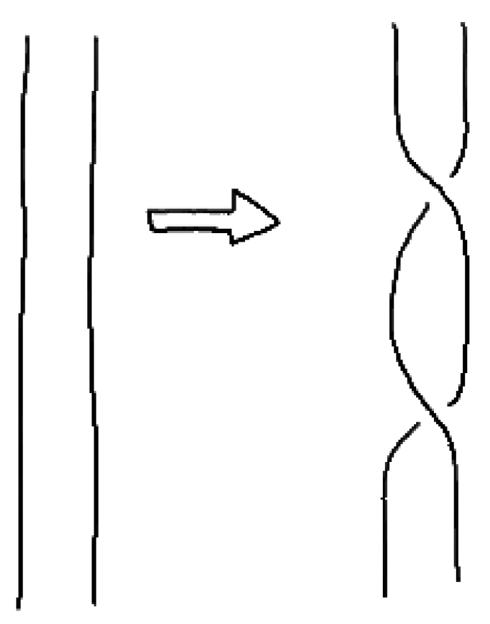
However, what does change in the knot complement and in the branched covering? As a toy example, we consider the complement of the unknot $D^2\times S^1$. Then, the Dehn twist along the meridian of the boundary torus will be trivialized. By a result of McCullough (see for instance [61]), every Dehn twist along the longitude induces a diffeomorphism of the solid torus. Then, the complement of the unknot can carry an electric charge (by a Dehn twist) but no magnetic charge. This result can be generalized to all knot complements (which are homologically equivalent to the solid torus). The effect on the branched covering can also be obtained by considering the boundary. The boundary is a torus written as two-fold branched covering branched along 4 points. A Dehn twist is given by a permutation of the branching points that leads to a twist of the braid as a branching set of the knot complement (see Figure 8).

We obtain again the quantization of the electric charge as the number of Dehn twists.

However, more is true: the isotopy classes of the boundary determine the isotopy classes of the hyperbolic knot complement up to a finite subgroup [59]. The mapping class group $MCG\left(C\right(K\left)\right)$ consists of a disjoint union of isotopy classes of framings, i.e., trivializations of the tangent bundle $TC\left(K\right)$ seen as sections of the frame bundle ($SO\left(3\right)$ principal bundle) up to homotopy. Therefore, the change of the number of Dehn twists at the boundary induces a change of the framing for the knot complement. However, there is also a direct way using obstruction theory. In [62], we described the quantization of the electric charge by using exotic smoothness as a substitute for a magnetic monopole. A magnetic monopole is a substitute for an element in the cohomology $H^2(S^2,\mathbb{Z})$ leading to the quantization of the electric charge

$$Q_m·Q_e=\frac{c\hslash }{2}·n,n\in \mathbb{Z}$$

for the magnetic charge $Q_m$ and for the electric charge $Q_e$. Using the canonical isomorphism

$$H^2(S^2,\mathbb{Z})\simeq H^3(S^3,\mathbb{Z}),$$

we can transform the monopole class (as first Chern class of a complex line bundle) into a class in $H^3(S^3,\mathbb{Z})$. Now, let P be a principal $SO\left(3\right)$ bundle over $S^3$, called the frame bundle. The obstruction for a section in this bundle lies at $H^4(S^3,{\pi }_3\left(SO\left(3\right)\right))=0$, where the vanishing of the cocycle guarantees the existence. The number of sections is given by the elements in $H^3(S^3,{\pi }_3\left(SO\left(3\right)\right))=H^3(S^3,\mathbb{Z})$ using ${\pi }_3\left(SO\left(3\right)\right)=\mathbb{Z}$. By Hodge duality, we obtain the same line of argumentation for the class $\ast F$ getting the electric charge (using also the quantization condition). The class in $H^3(S^3,\mathbb{Z})$ can be related to a relative class in the 4-manifold $S^3\times [0,1]$, i.e.,

$$H^3(S^3,\mathbb{Z})\simeq H^4(S^3\times [0,1],S^3\times \partial [0,1],\mathbb{Z})$$

called the relative Pontrjagin class $p_1$. Now, we extend the whole discussion to an arbitrary 3-manifold $\mathsf{\Sigma }$, which we identify with $\mathsf{\Sigma }=C\left(K\right)\cup (D^2\times S^1)$. Using this 4-dimensional interpretation, we obtain the framing as the Hirzebruch defect [63]. For that purpose, we consider the 4-manifold M with $\partial M=\mathsf{\Sigma }$. Let $\sigma \left(M\right)$ be the signature of M, i.e., the number of positive minus negative eigenvalues of the intersection form of M. Furthermore, let $p_1(M,\mathsf{\Sigma })$ be the relative Pontrjagin class as an element of $H^4(M,\partial M=\mathsf{\Sigma },\mathbb{Z})$. Then, the Hirzebruch defect h is given by

$$h=3\sigma \left(M\right)-p_1(M,\mathsf{\Sigma })=Q_e$$

(22)

and identified with the framing, i.e., with the charge. This definition is motivated by the Hirzebruchs signature formula for a closed 4-manifold relating the signature $\sigma \left(M\right)$ and the first Pontrjagin class $p_1\left(M\right)$ (of the tangent bundle $TM$) via $\sigma \left(M\right)=\frac{1}{3}{p}_1\left(M\right)$ (see [64]).

5.3. The Charge Spectrum

Now, we will discuss the expression (22) for the electric charge. By the argumentation above, the relative Pontrjagin class gives an integer expressing the framing of the knot complement for a fixed time. The appearance of the signature $\sigma \left(M\right)$ added a 4-dimensional element which describes more complex cases with many components. In [65], this case was also considered with a similar result: this formula is valid for links where $\sigma \left(M\right)$ is now the signature of the linking matrix and $p_1$ is the sum of framings for each component. The signature can be minimally changed by $\pm 1$ leading to a change of the charge by $\pm 3$. Therefore, the minimal change for one component can be

$$Q_{e}mod3\mathbb{Z}=\left\{0,\pm 1,\pm 2,\pm 3\right\},$$

i.e., we obtain a spectrum containing four possible values. If we normalize the charge to be a multiple of $e/3$, then we have the charge spectrum

$$Q_e=\left\{0,\pm \frac{1}{3}e,\pm \frac{2}{3}e,\pm e\right\}$$

in agreement with the experiment. Then, we have the description of one particle generation: two leptons (neutrino of charge 0 and lepton of charge $-1$) and two quarks (quark of charge $-\frac{1}{3}$ and quark of charge $+\frac{2}{3}$).

5.4. Vanishing of the Magnetic Charge and Quasimodularity

One may wonder whether there is no magnetic charge anymore. Our argument is only partially satisfying because there are many incompressible surfaces inside of a hyperbolic knot complement serving as representatives for magnetic charges. Therefore, we need a stronger argument why the symmetry between electric and magnetic charge is broken. As explained above, the Dehn twists of the boundary torus are the generators of the mapping class (or isotopy) group. According to Atiyah [63], the framing can be used to define a central extension $\widehat{\mathsf{\Gamma }}$

$$1\to \mathbb{Z}\to \widehat{\mathsf{\Gamma }}\to \mathsf{\Gamma }\to 1$$

of the mapping class group $\mathsf{\Gamma }$ so that there is a section $s:\mathsf{\Gamma }\to \widehat{\mathsf{\Gamma }}$ inducing a splitting of the sequence above. This section defines a canonical 2-cocycle c for the central extension that is given by the signature of the corresponding 4-manifold (see [63] for the details). However, in case of the torus, for the group $\mathsf{\Gamma }=SL(2,\mathbb{Z})$, there is no non-zero homomorphism $\mathsf{\Gamma }\to \mathbb{Z}$ and so the splitting $s_1:\mathsf{\Gamma }\to \widehat{\mathsf{\Gamma }}$ is unique. Therefore, the canonical section s is not a homomorphism and the framing (used in the definition of this section) leads to a breaking of the modular invariance i.e., the invariance w.r.t. $\mathsf{\Gamma }$. This fact is simply expressed by considering the difference of the two sections $s\left(\gamma \right)$ and $s_1\left(\gamma \right)$ for $\gamma \in \mathsf{\Gamma }$, which is given by the logarithm of the Dedekind $\eta -$function, related to quasimodular functions. Thus, our definition of the electric charge breaks explicitly the electro-magnetic duality and we get a vanishing magnetic charge.

6. Drinfeld–Turaev Quantization and Quantum States

In [66,67], we discussed the appearance of quantum states from knots known as Turaev–Drinfeld quantization. The idea for the following construction can be simply expressed. We start with two 3-manifolds and consider a cobordism between them. This cobordism is a 4-manifold with a branched covering branched over a surface with self-intersections. Here, it is enough to restrict to a special class of these surfaces, so-called ribbon surfaces (see [68]). The 3-manifolds are chosen to be hyperbolic knot complements, denoted by $Y_1,Y_2$. A hyperbolic structure is defined by a homomorphism ${\pi }_1\left(Y_i\right)\to SL(2,\mathbb{C})$ ($\in Hom({\pi }_1\left(Y_i\right),SL(2,\mathbb{C}))$) up to conjugation. Now, we extend this structure to the entire cobordism, denoted by $Cob(Y_1,Y_2)$. The branching set of $Cob(Y_1,Y_2)$ is a surface S with non-trivial fundamental group ${\pi }_1\left(S\right)$. This surface can be changed without any change of $Cob(Y_1,Y_2)$. One change can be described as crossing change. Now, we have all ingredients for the Drinfeld–Turaev quantization:

• The surface S (branching set of $Cob(Y_1,Y_2)$) is inducing a representation ${\pi }_1\left(S\right)\to SL(2,\mathbb{C})$.
• The space of all representations $X(S,SL(2,\mathbb{C}))=Hom({\pi }_1\left(S\right),SL(2,\mathbb{C}))/SL(2,\mathbb{C})$ has a natural Poisson structure (induced by the bilinear on the group) and the Poisson algebra $(X(S,SL(2,\mathbb{C}),\left\{\right\})$ of complex functions over them is the algebra of observables.
• The Skein module $K_{-1}(S\times [0,1])$ (i.e., $t=-1$) has the structure of an algebra isomorphic to the Poisson algebra $(X(S,SL(2,\mathbb{C})),\left\{\right\})$. (see also [69,70]).
• The skein algebra $K_t(S\times [0,1])$ is the quantization of the Poisson algebra $(X(S,SL(2,\mathbb{C})),\left\{\right\})$ with the deformation parameter $t=exp(h/4)$ (see also [69]) .

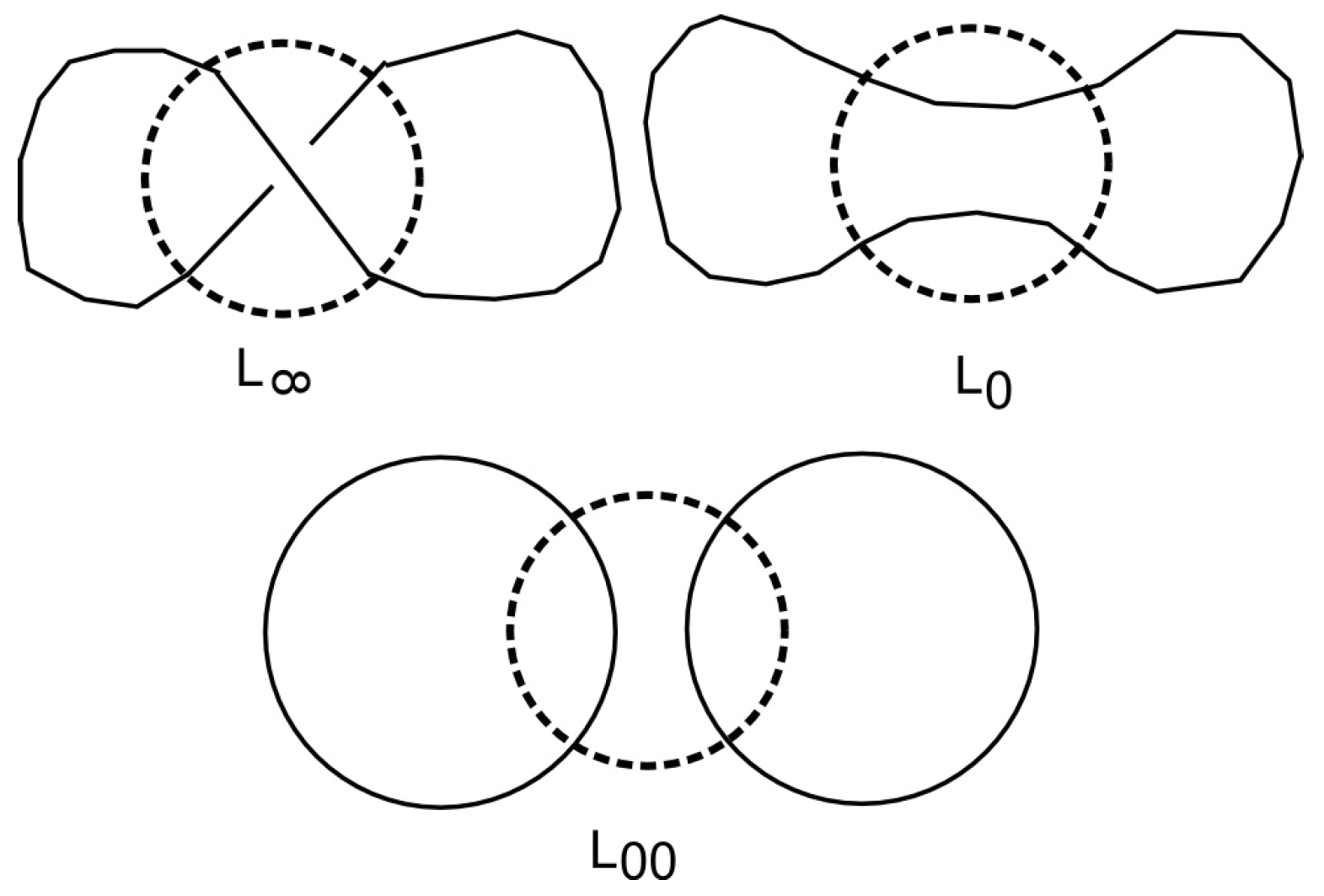
To understand these statements, we have to introduce the skein module $K_t\left(M\right)$ of a 3-manifold M (see [71]). For that purpose, we consider the set of links $\mathcal{L}\left(M\right)$ in M up to isotopy and construct the vector space $\mathbb{C}\mathcal{L}\left(M\right)$ with basis $\mathcal{L}\left(M\right)$. Then, one can define $\mathbb{C}\mathcal{L}\left[\right[t\left]\right]$ as ring of formal polynomials having coefficients in $\mathbb{C}\mathcal{L}\left(M\right)$. Now, we consider the link diagram of a link, i.e., the projection of the link to the ${\mathbb{R}}^2$ having the crossings in mind. Choose a disk in ${\mathbb{R}}^2$ so that one crossing is inside this disk. If the three links differ by the three crossings $L_{oo},L_o,L_{\infty }$ (see Figure 9) inside of the disk, then these links are skein related.

Then, in $\mathbb{C}\mathcal{L}\left[\right[t\left]\right]$, one writes the skein relation $L_{\infty }-t{L}_o-t^{-1}{L}_{oo}$ which depends only on the group $SL(2,\mathbb{C})$. Furthermore, let $L\bigsqcup O$ be the disjoint union of the link with a circle. Then, one writes the framing relation $L\bigsqcup O+(t^2+t^{-2})L$. Let $S\left(M\right)$ be the smallest submodule of $\mathbb{C}\mathcal{L}\left[\right[t\left]\right]$ containing both relations. Then, we define the Kauffman bracket skein module by $K_t\left(M\right)=\mathbb{C}\mathcal{L}\left[\left[t\right]\right]/S\left(M\right)$. The modification of S by using the skein relations is one of the allowed changes of the branching set to keep $Cob(Y_1,Y_2)$.

Now, we list the following general results about this module:

• The module $K_{-1}\left(M\right)$ for $t=-1$ is a commutative algebra.
• Let S be a surface. Then, $K_t(S\times [0,1])$ carries the structure of an algebra.

The algebra structure of $K_t(S\times [0,1])$ can be simply seen by using the diffeomorphism between the sum $S\times [0,1]{\cup }_{S}S\times [0,1]$ along S and $S\times [0,1]$. Then, the product $ab$ of two elements $a,b\in K_t(S\times [0,1])$ is a link in $S\times [0,1]{\cup }_{S}S\times [0,1]$ corresponding to a link in $S\times [0,1]$ via the diffeomorphism. The algebra $K_t(S\times [0,1])$ is in general non-commutative for $t\ne -1$. For the following, we will omit the interval $[0,1]$ and denote the skein algebra by $K_t\left(S\right)$.

As shown in [23,66,72], the skein algebra serves as the observable algebra of a quantum field theory. For this approach via branched coverings, the branching sets of knot complements (representing the fermions) are special braids (6-plats, see above). Any different braid is a different state or better than a different quantum state but not a different particle. As explained above, the charge spectrum is enough to describe one generation of particles (two leptons, two quarks). The appearance of different generations will be discussed below.

7. Fermions and Number Theory

In this section, we will present some ideas to uncover some explicit relations between fermions, given as hyperbolic knot complements, and number theory, notable quaternionic trace fields and algebraic K theory/Bloch group. However, we first need some definitions.

A quaternion algebra over a field ${\displaystyle F}$ is a four-dimensional central simple F-algebra. A quaternion algebra has a basis ${\displaystyle 1,i,j,ij}$ where ${\displaystyle i^2,j^2\in F^{\times }}$ and ${\displaystyle ij=-ji}$. A subgroup of ${\displaystyle \mathrm{PSL}(2,\mathbb{C})}$, the isometry group of the three-dimensional hyperbolic space isomorphic to the Lorentz group $SO(3,1)$, is said to be derived from a quaternion algebra if it can be obtained through the following construction. Let F be a number field that has exactly two embeddings into $\mathbb{C}$ whose image is not contained in $\mathbb{R}$. Let A be a quaternion algebra over ${\displaystyle F}$ such that, for any embedding ${\displaystyle \tau :F\to \mathbb{R}}$, the algebra ${\displaystyle A{\otimes }_{\tau }\mathbb{R}}$ is isomorphic to the quaternions. Let ${\displaystyle {\mathcal{O}}^1}$ be the group of elements in the order of A with a 1. An order of a quaternionic algebra A is a finitely generated submodule $\mathcal{O}$ of A of reduced norm 1 and let $\mathsf{\Gamma }$ be its image in the $2\times 2$ matrices $M_2\left(\mathbb{C}\right)$ via $\varphi :A\to M_2\left(\mathbb{C}\right).$ We then consider the Kleinian group obtained as the image in${\displaystyle \mathrm{PSL}(2,\mathbb{C})}$ of ${\displaystyle \varphi \left({\mathcal{O}}^1\right)}$. This subgroup is called an arithmetic Kleinian group. An arithmetic hyperbolic three-manifold is the quotient of hyperbolic space ${\displaystyle {\mathbb{H}}^3}$ by an arithmetic Kleinian group. The complement of the Figure 8 knot is one example of an arithmetic hyperbolic 3-manifold.

This class of 3-manifolds shows the strong relation between quaternions and 3-manifolds. We discussed above the relation between the K3 surface and the octonions. The starting point for the use of number theory in Kleinian groups is Mostow’s rigidity theorem. A consequence of this theorem is that the matrix entries in $SL(2,\mathbb{C})$ of a finite covolume Kleinian group $\mathsf{\Gamma }$ may be taken to lie in a number field that is a finite extension of $\mathbb{Q}$. However, it is true that there is a strong relation between certain number theoretic functions (Bloch–Wigner function, dilogarithm) and the volume of the hyperbolic 3-manifolds: the volume is the sum over all Bloch–Wigner functions for the ideal tetrahedrons forming this 3-manifold. For more information about the relation between hyperbolic 3-manifolds and number theory, consult the book [73]. We hope to use this relation in the future to obtain more properties of fermions by using number theory.

8. The K3 Surface and the Number of Generations

In Section 4.1, we discussed a relation between the K3 surface and octonions by using the intersection form. Here, we use only the $E_8$ matrix, i.e., the Cartan matrix of the Lie algebra $E_8$. In this section, we will speculate about the other part

$$H=\left(\begin{array}{cc}0& -1\\ -1& 0\end{array}\right)$$

of the intersection form (now with a different orientation). H is the intersection form of the 4-manifold $S^2\times S^2$. To express it explicitly, there are homology classes $\alpha ,\beta \in H_2(S^2\times S^2)$ with ${\alpha }^2={\beta }^2=0$ and $\alpha ·\beta =-1$. Therefore, every $S^2$ of this manifold has no self-intersections. For the topology of the K3 surface with intersection form (7), this form has the desired form, but, as explained above, we will change the smoothness structure. The central idea is the usage of Casson handles $CH$ for the 4-manifolds $S^2\times S^2\backslash pt$, the one-point complement of $S^2\times S^2$. Here, the homology classes $\alpha ,\beta$ are given (up to homotopy) by ${\alpha }^2,{\beta }^2=0mod2$ and $\alpha ·\beta =-1$; see [74]. However, then one has ${\alpha }^2=2n$. Interestingly, the existence of a spin structure is connected to the property that the squares of the homology classes are even. Here, we will consider the simplest realization which has non-zero squares, i.e., we get the form

$$\tilde{H}=\left(\begin{array}{cc}2& -1\\ -1& 2\end{array}\right).$$

(23)

This form cannot be an intersection form because $\tilde{H}$ has determinant 3. Therefore, only the $\tilde{H}mod2$ reduction has the meaning to be an intersection. However, for the moment, we will consider $\tilde{H}$ and apply the same construction as for the $E_8$, i.e., we see $\tilde{H}$ as the Cartan matrix for a Lie algebra. In this case, we get the Lie algebra of $SU\left(3\right)$ or the color group. The whole discussion uses some hand-waving arguments, but it is a sign that the $3\left(S^2\times S^2\right)$ part of the K3 surfaces is connected with the generations. Every part $S^2\times S^2$ has one color group and realizes the electric charge spectrum $0,\pm \frac{1}{3},\pm \frac{2}{3},\pm 1$. Thus, every $S^2\times S^2$ is the 4-dimensional expression for one generation. This result agrees with the discussion in [31] where we generate fermions from a Casson handle. Let us assume that the number of generations is given by the number of $S^2\times S^2$ summands. How many generations are possible? Here, we have the surprising result: if the underlying spacetime is a smooth manifold, then the minimal number of generations must be three! A spacetime with only one or two generations is not a smooth manifold. Then, the K3 surface is the minimal model.

We will close this paper with another speculation, a global symmetry induced from the K3 surface. Starting point is the intersection form again. From the point of number theory, this form is an even unimodular positive-definite lattices of rank 24, the so-called Niemeier lattice. In 2010, Eguchi–Ooguri–Tachikawa observed that the elliptic genus of the K3 surface decomposes into irreducible characters of the N = 4 superconformal algebra. The corresponding q-series is a mock modular form related to the sporadic group $M_{24}$, the Mathieu group, a simple group of order 244823040. The whole theory is known as Mathieu moonshine or umbral moonshine [75]. The interesting point here is the maximal subgroup of $M_{24}$, the split extension of $PGL(3,4)$ by $S_3$. The group is the projective group of $3\times 3$ matrices with values in the field of four elements. It seems that this maximal subgroup acts in some sense on the K3 surface, and we conjecture that this group acts on the $S^2\times S^2$ part. If our idea of a relation between the three generations and the $3\left(S^2\times S^2\right)$ part of the K3 surfaces is true, then we hope to get the mixing matrix for quarks and neutrinos from this action.

9. Conclusions and Outlook

In this paper, we presented a top-down approach to fermions and bosons, in particular the standard model. What was done in the paper?

• We constructed a spacetime, the K3 surface and derive some numbers like the cosmological constant or some energy scales and neutrino masses agreeing with experimental data.
• We derived from a representation of K3 surfaces by branched covering a simple picture: fermions are hyperbolic knot complements, whereas bosons are link complements (torus bundles).
• We obtained the gauge group from this picture (at least in principle).
• We derived the correct charge spectrum and obtained one generation.
• We conjectured about the number of generations and global symmetry (the $PGL(3,4)$) to get the mixing between the generations.

What are the consequences for physics? The model only has a few direct consequences. We introduced fermions and bosons in a geometric way. Except for the right-handed neutrino (needed for the see-saw mechanism to generate the masses), we only got the fermions and gauge bosons of the standard model. No extension is needed. The usage of torus bundles for the gauge bosons should generate additional relations for the corresponding scattering amplitudes. The appearance of the global symmetry $PGL(3,4)$ should be related the mixing of quarks and neutrinos. In [40], we also discussed the appearance of an asymmetry between particles and anti-particles induced by the topology of the spacetime. This idea is also valid in this model, but we cannot match it to the observations.

Is there an outline on some new experiments derived by this model? Currently, this model makes some predictions about the neutrino masses, charge spectrum and the existence of a right-handed neutrino. However, these predictions can be checked by a better measurement in known experiments. Now, there are no new ideas about special experiments connected with this model.

Among these results, there are, of course, many open points of the kind: what is the color and weak charge? How can we implement the Higgs mechanism? What is mass? For the Higgs mechanism, we had found a possible scheme in our previous work [40,76], but it is only a beginning. Many aspects of this paper are related to the ideas of Furey and Gresnigt. It is a future project to extend it and bridge our approach with these ideas.

References

- Collaborations, F.G. Testing Einstein’s Special Relativity with Fermi’s Short Hard Gamma-Ray Burst GRB090510. Nature 2009, 462, 331–334. [Google Scholar]
- Furey, C. Towards a Unified Theory of Ideals. Phys. Rev. D 2012, 86, 025024. [Google Scholar] [CrossRef]
- Furey, C. Generations: Three Prints, in Colour. JHEP 2014, 10, 046. [Google Scholar] [CrossRef]
- Furey, C. Charge Quantization from a Number Operator. Phys. Lett. B 2015, 742, 195–199. [Google Scholar] [CrossRef]
- Furey, C. Standard Model Physics from an Algebra? Ph.D. Thesis, University of Waterloo, Waterloo, ON, Canada, 2015. Available online: https://arxiv.org/abs/1611 (accessed on 1 October 2019).
- Gresnigt, N. Braids, Normed Division Algebras, and Standard Model Symmetries. Phys. Lett. B 2018, 783, 212–221. [Google Scholar] [CrossRef]
- Gresnigt, N. Braided Fermions from Hurwitz Algebras. J. Phys. Conf. Ser. 2019, 1194, 012040. [Google Scholar] [CrossRef]
- Gillard, A.; Gresnigt, N. Three Fermion Generations with Two Unbroken Gauge Symmetries from the Complex Sedenions. Eur. Phys. J. C 2019, 79, 446. [Google Scholar] [CrossRef]
- Stoica, O. Leptons, Quarks, and Gauge from the Complex Clifford Algebra Cℓ6. Adv. Appl. Cliff. Alg. 2018, 28, 52. [Google Scholar] [CrossRef]
- Thomson, W. On Vortex Motion. Trans. R. Soc. Ed. 1869, 25, 217–260. [Google Scholar] [CrossRef]
- Misner, C.; Thorne, K.; Wheeler, J. Gravitation; Freeman: San Francisco, CA, USA, 1973. [Google Scholar]
- Mielke, E. Knot Wormholes in Geometrodynamics? Gen. Relat. Grav. 1977, 8, 175–196. [Google Scholar] [CrossRef]
- Giulini, D. Matter from Space. Based on a talk delivered at the conference “Beyond Einstein: Historical Perspectives on Geometry, Gravitation, and Cosmology in the Twentieth Century”, September 2008 at the University of Mainz in Germany. To appear in the Einstein-Studies Series, Birkhaeuser, Boston. arXiv 2008, arXiv:0910.2574. [Google Scholar]
- Jehle, H. Topological characterization of leptons, quarks and hadrons. Phys. Lett. B 1981, 104, 207–211. [Google Scholar] [CrossRef]
- Gavrilik, A.M. Quantum algebras in phenomenological description of particle properties. Nucl. Phys. B (Proc. Suppl.) 2001, 102/103, 298–305. [Google Scholar] [CrossRef]
- Finkelstein, R. Knots and Preons. Int. J. Mod. Phys. A 2009, 24, 2307–2316. [Google Scholar] [CrossRef]
- Bilson-Thompson, S. A Topological Model of Composite Preons. arXiv 2005, arXiv:0503213v2. [Google Scholar]
- Bilson-Thompson, S.; Markopoulou, F.; Smolin, L. Quantum Gravity and the Standard Model. Class. Quant. Grav. 2007, 24, 3975–3994. [Google Scholar] [CrossRef]
- Duston, C. Exotic Smoothness in 4 Dimensions and Semiclassical Euclidean Quantum Gravity. Int. J. Geom. Meth. Mod. Phys. 2010, 8, 459–484. [Google Scholar] [CrossRef]
- Duston, C.L. Topspin Networks in Loop Quantum Gravity. Class. Quant. Grav. 2012, 29, 205015. [Google Scholar] [CrossRef]
- Duston, C.L. The Fundamental Group of a Spatial Section Represented by a Topspin Network. Based on Work Presented at the LOOPS 13 Conference at the Perimeter Institute. arXiv 2013, arXiv:1308.2934. [Google Scholar]
- Denicola, D.; Marcolli, M.; al Yasry, A. Spin Foams and Noncommutative Geometry. Class. Quant. Grav. 2010, 27, 205025. [Google Scholar] [CrossRef]
- Asselmeyer-Maluga, T. Smooth Quantum Gravity: Exotic Smoothness and Quantum Gravity. In At the Frontiers of Spacetime: Scalar-Tensor Theory, Bell’s Inequality, Mach’s Principle, Exotic Smoothness; Asselmeyer-Maluga, T., Ed.; Springer: Basel, Switzerland, 2016. [Google Scholar]
- Rolfson, D. Knots and Links; Publish or Prish: Berkeley, CA, USA, 1976. [Google Scholar]
- Hilden, H. Every Closed Orientable 3-Manifold is a 3-Fold Branched Covering Space of S3. Bull. Am. Math. Soc. 1974, 80, 1243–1244. [Google Scholar] [CrossRef]
- Hirsch, U. Über Offene Abbildungen Auf Die 3-Sphäre. Math. Z. 1974, 140, 203–230. [Google Scholar] [CrossRef]
- Montesinos, J. A Representation of Closed, Orientable 3-Manifolds as 3-Fold Branched Coverings of S3. Bull. Am. Math. Soc. 1974, 80, 845–846. [Google Scholar] [CrossRef]
- Piergallini, R. Four-Manifolds as 4-Fold Branched Covers of S4. Topology 1995, 34, 497–508. [Google Scholar] [CrossRef]
- Iori, M.; Piergallini, R. 4-Manifolds as Covers of S4 Branched over Non-Singular Surfaces. Geom. Topol. 2002, 6, 393–401. [Google Scholar] [CrossRef]
- Piergallini, R.; Zuddas, D. On Branched Covering Representation of 4-Manifolds. J. Lond. Math. Soc. 2018, 99. in press. [Google Scholar] [CrossRef]
- Asselmeyer-Maluga, T.; Brans, C. How to Include Fermions Into General Relativity by Exotic Smoothness. Gen. Relat. Grav. 2015, 47, 30. [Google Scholar] [CrossRef]
- Asselmeyer-Maluga, T.; Rosé, H. On the Geometrization of Matter by Exotic Smoothness. Gen. Relat. Grav. 2012, 44, 2825–2856. [Google Scholar] [CrossRef]
- Brans, C. Localized exotic smoothness. Class. Quant. Grav. 1994, 11, 1785–1792. [Google Scholar] [CrossRef] [Green Version]
- Brans, C. Exotic smoothness and physics. J. Math. Phys. 1994, 35, 5494–5506. [Google Scholar] [CrossRef] [Green Version]
- Yau, S.T. On the Ricci Curvature of a Compact Kähler Manifold and the Complex Monge-Ampère Equation. Commun. Pure Appl. Math. 1978, 31, 339–411. [Google Scholar] [CrossRef]
- LeBrun, C. Four-Manifolds Without Einstein Metrics. Math. Res. Lett. 1996, 3, 133–147. [Google Scholar] [CrossRef]
- Asselmeyer-Maluga, T.; Król, J. On Topological Restrictions of the Spacetime in Cosmology. Mod. Phys. Lett. A 2012, 27, 1250135. [Google Scholar] [CrossRef]
- Donaldson, S. An Application of Gauge Theory to the Topology of 4-Manifolds. J. Diff. Geom. 1983, 18, 269–316. [Google Scholar] [CrossRef]
- Asselmeyer-Maluga, T.; Krol, J. How to Obtain a Cosmological Constant from Small Exotic R4. Phys. Dark Universe 2018, 19, 66–77. [Google Scholar] [CrossRef]
- Asselmeyer-Maluga, T.; Krol, J. A Topological Approach to Neutrino Masses by Using Exotic Smoothness. Mod. Phys. Lett. A 2019, 34, 1950097. [Google Scholar] [CrossRef]
- Asselmeyer-Maluga, T.; Krol, J. A Topological Model for Inflation. arXiv 2018, arXiv:1812.08158. [Google Scholar]
- Whitt, B. Fourth Order Gravity as General Relativity Plus Matter. Phys. Lett. 1984, 145B, 176–178. [Google Scholar] [CrossRef]
- Starobinski, A. A New Type of Isotropic Cosmological Models Without Singularity. Phys. Lett. B 1980, 91, 99–102. [Google Scholar] [CrossRef]
- Gompf, R.; Stipsicz, A. 4-Manifolds and Kirby Calculus; American Mathematical Society: Providence, RI, USA, 1999. [Google Scholar]
- Ade, P.A.; Aghanim, N.; Armitage-Caplan, C.; Arnaud, M.; Ashdown, M.; Atrio-Barandela, F.; Aumont, J.; Baccigalupi, C.; Banday, A.J.; Barreiro, R.B.; et al. Planck 2013 Results. XVI. Cosmological Parameters. Astron. Astrophys. 2013, 571, A16. [Google Scholar]
- Ade, P.C.P.; Aghanim, N.; Arnaud, M.; Ashdown, M.; Aumont, J.; Baccigalupi, C.; Banday, A.J.; Barreiro, R.B.; Bartlett, J.G.; Bartolo, N. Planck 2015 Results. XIII Cosmological Parameters. Astron. Astrophys. 2016, 594, A13. [Google Scholar]
- Bonvin, V.; Courbin, F.; Suyu, S.H.E.A. H0LiCOW-V. New COSMOGRAIL Time Delays of HE 0435-1223: H0 to 3.8 Per Cent Precision from Strong Lensing in a Flat ΛCDM Model. Mon. Not. R. Astron. Soc. 2016, 465, 4914–4930. [Google Scholar] [CrossRef]
- Asselmeyer-Maluga, T.; Król, J. Inflation and Topological Phase Transition Driven by Exotic Smoothness. Adv. HEP 2014, 14. [Google Scholar] [CrossRef]
- Freedman, M. The topology of four-dimensional manifolds. J. Diff. Geom. 1982, 17, 357–454. [Google Scholar] [CrossRef]
- Coxeter, H. Integral Caleay Numbers. Duke Math. J. 1946, 13, 561–578. [Google Scholar] [CrossRef]
- Friedrich, T. On the Spinor Representation of Surfaces in Euclidean 3-Space. J. Geom. Phys. 1998, 28, 143–157. [Google Scholar] [CrossRef]
- Ashtekar, A.; Engle, J.; Sloan, D. Asymptotics and Hamiltonians in a First, Order Formalism. Class. Quant. Grav. 2008, 25, 095020. [Google Scholar] [CrossRef]
- Ashtekar, A.; Sloan, D. Action and Hamiltonians in Higher Dimensional General Relativity: First, Order Framework. Class. Quant. Grav. 2008, 25, 225025. [Google Scholar] [CrossRef]
- Floer, A. An instanton Invariant for 3-manifolds. Commun. Math. Phys. 1988, 118, 215–240. [Google Scholar] [CrossRef]
- Calegari, D. Foliations and the Geometry of 3-Manifolds; Oxford University Press: Oxford, UK, 2007. [Google Scholar]
- Thurston, W. Three-Dimensional Geometry and Topology, 1st ed.; Princeton University Press: Princeton, NJ, USA, 1997. [Google Scholar]
- Giulini, D. Properties of 3-Manifolds for Relativists. Int. J. Theor. Phys. 1994, 33, 913–930. [Google Scholar] [CrossRef]
- Kalliongis, J.; McCullough, D. Isotopies of 3-Manifolds. Top. Appl. 1996, 71, 227–263. [Google Scholar] [CrossRef]
- Hatcher, A.; McCullough, D. Finiteness of Classifying Spaces of Relative Diffeomorphism Groups of 3-Manifolds. Geom. Top. 1997, 1, 91–109. Available online: http://www.math.cornell.edu/~hatcher/Papers/bdiffrel.pdf (accessed on 1 October 2019). [CrossRef]
- Giveon, A.; Kutasov, D. Brane Dynamics and Gauge Theory. Rev. Mod. Phys. 1999, 71, 983–1084. [Google Scholar] [CrossRef]
- Hong, S.; McCullough, D. Mapping Class Groups of 3-Manifolds, Then and Now. In Geometry and Topology Down Under; Hodgson, C.D., Jaco, W.H., Scharlemann, M.G., Tillmann, S., Eds.; AMS: Providence, RI, USA, 2013; Volume 597. [Google Scholar]
- Asselmeyer-Maluga, T.; Król, J. Abelian Gerbes, Generalized Geometries and Foliations of Small Exotic R4. arXiv 2014, arXiv:0904.1276v5. [Google Scholar]
- Atiyah, M. On Framings of 3-Manifolds. Topology 1990, 29, 1–7. [Google Scholar] [CrossRef]
- Hirzebruch, F. Topological Methods in Algebraic Geometry; Springer: Berlin/Heidelberg, Germany; New York, NY, USA, 1973. [Google Scholar]
- Freed, D.; Gompf, R. Computer calculation of Witten’s 3-manifold invariant. Commun. Math. Phys. 1991, 141, 79–117. [Google Scholar] [CrossRef]
- Asselmeyer-Maluga, T.; Król, J. Quantum Geometry and Wild Embeddings as Quantum States. arXiv 2013, arXiv:1211.3012. [Google Scholar] [CrossRef]
- Asselmeyer-Maluga, T. Hyperbolic Groups, 4-Manifolds and Quantum Gravity. J. Phys. Conf. Ser. 2019, 1194, 012009. [Google Scholar] [CrossRef]
- Piergallini, R.; Zuddas, D. A Universal Ribbon Surface in B4. Proc. Lond. Math. Soc. 2005, 90, 763–782. [Google Scholar] [CrossRef]
- Bullock, D.; Przytycki, J. Multiplicative Structure of Kauffman Bracket Skein Module Quantization. Proc. AMS 1999, 128, 923–931. [Google Scholar] [CrossRef]
- Bullock, D. A Finite Set of Generators for the Kauffman Bracket Skein Algebra. Math. Z. 1999, 231, 91–101. [Google Scholar] [CrossRef]
- Prasolov, V.; Sossinisky, A. Knots, Links, Braids and 3-Manifolds; AMS: Providence, RI, USA, 1997. [Google Scholar]
- Asselmeyer-Maluga, T.; Mader, R. Exotic R4 and Quantum Field Theory. In Proceedings of the 7th International Conference on Quantum Theory and Symmetries (QTS7), Prague, Czech Republic, 7–13 August 2011; Al, C.B.E., Ed.; IOP Publishing: Bristol, UK, 2012; p. 012011. [Google Scholar] [CrossRef]
- Maclachlan, C.; Reid, A.W. The Arithmetic of Hyperbolic 3-Manifolds; Springer Publisher: New York, NY, USA, 2003; Volume 219. [Google Scholar]
- Casson, A. Three Lectures on New Infinite Constructions in 4-Dimensional Manifolds, Progress in Mathematics ed.; Notes by Lucian Guillou; Birkhauser Boston: Boston, MA, USA, 1986; Volume 62. First Published 1973. [Google Scholar]
- Cheng, M.; Duncan, J.; Harvey, J. Umbral Moonshine and the Niemeier Lattices. Res. Math. Sci. 2014, 1, 3. [Google Scholar] [CrossRef]
- Asselmeyer-Maluga, T.; Król, J. Higgs Potential and Confinement in Yang-Mills Theory on Exotic R4. arXiv 2013, arXiv:1303.1632. [Google Scholar]
Figure 1.
2-fold covering of torus, is the equator and the four-point branching set.
Figure 2.
Branching set changes, Left: Move 1, Right: Move 2 (so-called Montesino moves).
Figure 3.
Boundary of the branching set change—Left: Move 1 leading to the Trefoil knot, Right: Move 2 leading to the Hopf link.
Figure 4.
3-fold covering torus.
Figure 5.
Covering of the handle body.
Figure 6.
Left: branching set of knot complement (6-plat), Right: 3-Braid as 6-Braid.
Figure 7.
Branching sets—Left: 6-Plat for the knot cpomplement, Center: a 3-Braid as 6-Braid as example, Right: 6-Braid for the link complement
Figure 8.
Dehn twist represented by a braid.
Figure 9.
Crossings
© 2019 by the author. Licensee MDPI, Basel, Switzerland. This article is an open access article distributed under the terms and conditions of the Creative Commons Attribution (CC BY) license (http://creativecommons.org/licenses/by/4.0/).
Share and Cite
MDPI and ACS Style
Asselmeyer-Maluga, T. Braids, 3-Manifolds, Elementary Particles: Number Theory and Symmetry in Particle Physics. Symmetry 2019, 11, 1298. https://doi.org/10.3390/sym11101298
AMA Style
Asselmeyer-Maluga T. Braids, 3-Manifolds, Elementary Particles: Number Theory and Symmetry in Particle Physics. Symmetry. 2019; 11(10):1298. https://doi.org/10.3390/sym11101298
Chicago/Turabian StyleAsselmeyer-Maluga, Torsten. 2019. "Braids, 3-Manifolds, Elementary Particles: Number Theory and Symmetry in Particle Physics" Symmetry 11, no. 10: 1298. https://doi.org/10.3390/sym11101298
Note that from the first issue of 2016, this journal uses article numbers instead of page numbers. See further details here.