Another View of Aggregation Operators on Group-Based Generalized Intuitionistic Fuzzy Soft Sets: Multi-Attribute Decision Making Methods

Abstract

In this paper, the existing definition of the group-based generalized intuitionistic fuzzy soft set is clarified and redefined by merging intuitionistic fuzzy soft set over the set of alternatives and a group of intuitionistic fuzzy sets on parameters. In this prospect, two new subsets of the group-based generalized intuitionistic fuzzy soft set are proposed and several operations are contemplated. The two new aggregation operators called generalized group-based weighted averaging and generalized group-based weighted geometric operator are introduced. The related properties of proposed operators are discussed. The recent research is emerging on multi-attribute decision making methods based on soft sets, intuitionistic fuzzy soft sets, and generalized intuitionistic fuzzy soft sets. An algorithm is structured and two case studies of multi-attribute decision makings are considered using proposed operators. Further, we provide the comparison and advantages of the proposed method, which give superiorities over recent major existing methods.

1. Introduction

The concept of fuzzy soft sets was popularized by Maji et al. [1], in the combination of fuzzy sets (Zadeh [2]) and soft sets (Molodtsov [3], Maji [4] and Ali [5]). To analyze the real-life problems, different types of uncertainties have been evaluated with fuzzy soft sets [6] and it has wide range of applications to deal with parameterizations and granularity. By virtue of robustness of fuzzy soft set theory in dealing with uncertain data, many researchers serve to integrate it with inductive learning techniques for better results. In recent past, fuzzy sets, soft sets and fuzzy soft sets are applied to evaluate vagueness in decision makings [7,8,9,10,11,12,13,14,15,16,17,18], algebraic structures [19,20], medical diagnosis [21] and differential equations [22]. Some hybrid models of fuzzy soft sets have been introduced and applied in several fields [23,24].

In 1986, Atanassov proposed the intuitionistic fuzzy set (IFS) [25], which appears as an inclusion of non-compatibility value with fuzzy set [2]. Every value of IFS is referred to a compatibility, a non-compatibility and a hesitancy, which assign it more dynamics in dealing with imprecise information. The initial aggregation instruments [26,27] on IFSs were introduced by Atanassov and Xu, and then applied in a various fields. The geometric [28], and arithmetic aggregation operators [27] have been studied in diverse fields and especially in multi-attribute decision making (MADM) problems in financial management, medical diagnosis, business and engineering designs [29,30,31,32].

IFSs with soft sets, that is, intuitionistic fuzzy soft sets (IFSSs) [33], are very instrumental and more realistic tools for uncertainty than fuzzy soft sets. As the dual-memberships structure of IFS allow marking hesitancy factors, the use of IFSSs in inductive learning techniques accounts for the degree of imprecision by assigning grades of compatibility and non-compatibility. In an inclusive way, several decision-making problems have been considered using IFSSs; some attempts are hybrid with intervals [34], multi-attributes [35] and nonlinear-programming [36]. Garg et al. [37,38] popularized aggregation operators on IFSSs and considered related decision-making methods. Several strategies are used to overcome the challenges of granularity and vagueness. Despite there being the applicability of IFSSs in diverse fields, an opinion of an expert who implicitly exercises his assessments on parameters of an IFSS is needed. On this motivation, Agarwal et al [39], who popularized generalized intuitionistic fuzzy soft set (GIFSS) by including assessment of a moderator on parameters, thus validating and supporting the information. Thus, the accumulation of generalized parameter can reduce possibility of errors which are occur due to imprecise data.

Although the definition of GIFSS in [39] is useful to tackle imprecise data, some difficulties appear in several notions [40,41]. Altogether, the assertions in [39] have been pointed out and a novel definition of GIFSS was established by Feng et al. [42]. They presented several operations and developed related multi-attribute decision-making methods by introducing operators on GIFSSs. On this prospect, a practical application of GIFSS for design concept evaluation was proposed by Hayat et al. [43]. Even though GIFSSs are applicable in diverse fields, sometimes assessments of more than one prospectors are needed in various problems. Thus, we consider the problem of validation of the notion of group-based GIFSS (GGIFSS) [44,45], and introduce a novel definition of GGIFSS, which is the generalization of the notion of GIFSS in [42]. Further, some basic properties are validated and aggregation instruments are proposed to determine the industrial applicability of GGIFSSs. Usually, an accurate aggregation process recommends the nature of MCDM model, which aggregates interdependent information and behaves in a linear manner. The prospect of proposing group-based generalized weighted averaging and geometric operators (hereafter, GBGWA and GBGWG) is to contemplate the information together with the influence of mathematical operations on GGIFSSs. The advantages of the given framework are to contemplate the prospector’s demands or experts’ judgments in an incorporated way such that establishing more operators constitutes the design concept of the evaluation mechanism of GGIFSSs.The results presented in this paper can be studied in several fields, such as electrical engineering, industrial designs, and construction engineering, as estimation of risk factors in risk management is a complex tasks.

The paper is organized as follows. Section 2 introduce basic concepts and notations. Section 3 clarify and redefine the notion of GGIFSS. Section 4 give operations on GGIFSSs, and introduce GBGWA(GBGWG) operators and related properties. Section 5 put forward the aggregation instruments of GGIFSSs into algorithm and discuss two different case studies. We present the comparison and benefits of method in Section 6. Advantages and superiorities are given in Section 7. Section 8 provide the conclusions of the paper.

2. Preliminaries

In this section, we present the basic definitions of fuzzy sets, IFSs, soft sets and GIFSS which would be useful for subsequent discussions. Throughout the paper, X is the universe.

A fuzzy set $\tilde{t}$ in X is usually identified as its membership function $\tilde{t}:X⟶[0,1]$ [2], each $x\in X$, where the membership grade $\tilde{t}(x)$ indicates the degree to which the element x belongs to the fuzzy set $\tilde{t}$. Here, we denote by $\mathcal{F}(X)$ the collection of all fuzzy sets in X. The subsets intersection, union and complement of fuzzy sets follow from Zadeh [2].

In 1999, Molodtsov [3] introduced the parameterization concept soft set theory, which is different from many traditional tools for dealing with uncertainties, such as fuzzy set theory [2], rough set theory [46], IFSs [25], and hesitant fuzzy sets. The main advantage of soft set theory is that it can be freely applied to characterized parameters, sentence, words and numbers. The natural manner of parameterization of this theory was augmented by the works of Maji et al. [4] and Ali et al. [5], among others.

Definition 1.

[3] Let E be the set of parameters, $\mathcal{A}\subseteq E$. A pair $(\mathcal{S},\mathcal{A})$ is called a soft set over X, where $\mathcal{S}$ is a mapping given by $\mathcal{S}:\mathcal{A}⟶P(X)$. $P(X)$ is the set of all power sets of X.

The set of all soft sets over X, with respect to subsets of E, is denoted by ${\mathcal{SASS}}^E(X)$.

2.1. Intuitionistic Fuzzy Sets

In the fuzzy set, only one compatibility degree exists, whereas intellectual insight in many cases suggests that non-compatibility degrees should be paired with compatibility degree. Atanassov [25] introduced the concept of IFS, which is an intellectual intuition to judge the uncertainty over the objects. Atanassov gave the definition of the IFS as follows:

Definition 2.

[25] An intuitionistic fuzzy set $(IFS)$ in a universe X is defined as

$$\mathcal{A}=\{\langle x,{\tilde{t}}_{\mathcal{A}}(x),{\tilde{f}}_{\mathcal{A}}(x)\rangle \mid x\in X\},$$

where the functions $\tilde{t},\tilde{f}:X⟶[0,1]$ define, respectively, a membership function and a non-membership function of the element $x\in X$ to the set $\mathcal{A}$. Moreover, it is required that

$$0\le {\tilde{t}}_{\mathcal{A}}(x)+{\tilde{f}}_{\mathcal{A}}(x)\le 1.$$

The function ${\pi }_{\mathcal{A}}=1-({\tilde{t}}_{\mathcal{A}}(x)+{\tilde{f}}_{\mathcal{A}}(x))$ is called the degree of hesitancy of x to $\mathcal{A}$. The collection of all IFSs in X is denoted by $IFS(X)$.

Let $\mathcal{A}$, $\mathcal{B}\in IFS(X)$. Then,

$$\mathcal{A}\bigsqcup \mathcal{B}=\{\langle x,max\{{\tilde{t}}_{\mathcal{A}}(x),{\tilde{t}}_{\mathcal{B}}(x)\},min\{{\tilde{f}}_{\mathcal{A}}(x),{\tilde{f}}_{\mathcal{B}}(x)\}\rangle \mid x\in X\},$$

$$\mathcal{A}\sqcap \mathcal{B}=\{\langle x,min\{{\tilde{t}}_{\mathcal{A}}(x),{\tilde{t}}_{\mathcal{B}}(x)\},max\{{\tilde{f}}_{\mathcal{A}}(x),{\tilde{f}}_{\mathcal{B}}(x)\}\rangle \mid x\in X\},$$

$$\mathcal{A}⊑\mathcal{B}\iff {\tilde{t}}_{\mathcal{A}}(x)\le {\tilde{t}}_{\mathcal{B}}(x) \mathrm{and} {\tilde{f}}_{\mathcal{A}}(x)\ge {\tilde{f}}_{\mathcal{B}}(x)\forall x\in X.$$

Deschrijver and Kerre [47] defined that IFSs can be considered as L-fuzzy sets with respect to the complete lattice $(V^{*},{⩽}_{V^{*}})$, where $V^{*}=\{\langle {\mu }_1,{\mu }_2\rangle \in {[0,1]}^2\mid {\mu }_1+{\mu }_2\le 1\},$ and the corresponding partial order ${⩽}_{V^{*}}$ is defined as $\langle {\mu }_1,{\mu }_2\rangle {⩽}_{V^{*}}\langle {\nu }_1,{\nu }_2\rangle \iff ({\mu }_1\le {\nu }_1)\wedge ({\mu }_2\le {\nu }_2)$ for all $\langle {\mu }_1,{\mu }_2\rangle ,\langle {\nu }_1,{\nu }_2\rangle \in V^{*}$. Any ordered pair $\langle {\mu }_1,{\mu }_2\rangle \in V^{*}$ is called an intuitionistic fuzzy value (IFV) or intuitionistic fuzzy number (IFN).

Let $V^{*}$ be the set of IFVs of IFS $\mathcal{A}$, such that $\langle {\tilde{t}}_{\mathcal{A}},{\tilde{f}}_{\mathcal{A}}\rangle \in V^{*}$. Chen and Tan [48] presented score function, which was updated by Feng et al. [42] as follows:

Definition 3.

[42] Let $\langle {\tilde{t}}_{\mathcal{A}},{\tilde{f}}_{\mathcal{A}}\rangle \in V^{*}$ be an IFV in a universe X. Then, expectation score function is a mapping $\delta :V^{*}\to [0,1]$, defined as follows:

$${\delta }_{\mathcal{A}}=\frac{{\tilde{t}}_{\mathcal{A}}-{\tilde{f}}_{\mathcal{A}}+1}{2}$$

(1)

where ${\delta }_{\mathcal{A}}$ is called the decision value of $\langle {\tilde{t}}_{\mathcal{A}},{\tilde{f}}_{\mathcal{A}}\rangle$ in $\mathcal{A}$. In addition, fuzzy set ${\delta }_{\mathcal{A}}$ is called the utility fuzzy set derived from the IFS $\mathcal{A}$.

Definition 4.

[28] Let $V_1=\langle {\tilde{t}}_{\mathcal{A}},{\tilde{f}}_{\mathcal{A}}\rangle ,V_2=\langle {\tilde{t}}_{\mathcal{A}}^{\prime },{\tilde{f}}_{\mathcal{A}}^{\prime }\rangle \in V^{*}$ be two IFVs in a universe X. Then we have,

(i)

$V_1\oplus V_2=\langle {\tilde{t}}_{\mathcal{A}}+{\tilde{t}}_{\mathcal{A}}^{\prime }-{\tilde{t}}_{\mathcal{A}}{\tilde{t}}_{\mathcal{A}}^{\prime },{\tilde{f}}_{\mathcal{A}}{\tilde{f}}_{\mathcal{A}}^{\prime }\rangle$.

(ii)

$V_1\otimes V_2=\langle {\tilde{t}}_{\mathcal{A}}{\tilde{t}}_{\mathcal{A}}^{\prime },{\tilde{f}}_{\mathcal{A}}+{\tilde{f}}_{\mathcal{A}}^{\prime }-{\tilde{f}}_{\mathcal{A}}{\tilde{f}}_{\mathcal{A}}^{\prime }\rangle$.

(iii)

$ϵV_1=\langle 1-{(1-{\tilde{t}}_{\mathcal{A}})}^{ϵ},{({\tilde{f}}_{\mathcal{A}})}^{ϵ}\rangle$, where ϵ is a positive real number.

More operations and properties of IFVs (or IF numbers (IFNs)) can be seen in [27,28,42]. Let $c_1,c_2,\dots ,c_m$ be the IFVs and $\varphi =({\varphi }_1,{\varphi }_2,\dots ,{\varphi }_m)$ be the correlated weighted normalized vector, then, from Yager [28] and Xu [27], we denote and symbolize the following operators:

$$\mathrm{IFWA}(c_1,c_2,\dots ,c_m)={\varphi }_1{c}_1\otimes {\varphi }_2{c}_3\otimes ,\dots ,\otimes {\varphi }_m{c}_m=\langle 1-\prod _i^m{(1-{\tilde{t}}_{c_i})}^{{\varphi }_i},\prod _i^m{\tilde{f}}_{c_i}^{{\varphi }_i}\rangle ,$$

(2)

$$\mathrm{IFWG}(c_1,c_2,\dots ,c_m)=c_1^{{\varphi }_1}\otimes c_3^{{\varphi }_3}\otimes ,\dots ,\otimes c_m^{{\varphi }_m}=\langle \prod _i^m{\tilde{t}}_{c_i}^{{\varphi }_i},1-\prod _i^m{(1-{\tilde{f}}_{c_i})}^{{\varphi }_i}\rangle .$$

(3)

IFWA and IFWG are the IF weighted averaging and geometric operators, respectively.

2.2. Intuitionistic Fuzzy Soft Sets and Generalized Intuitionistic Fuzzy Soft Sets

In this section, we present some basic notions in the theory of IFSS and GIFSS. The notion of IFSS is given as follows:

Definition 5.

[33] Let $(X,E)$ be a soft universe and $\mathcal{A}\subseteq E$. A pair $\mathcal{F}=(\tilde{\mathcal{S}},\mathcal{A})$ is called intuitionistic fuzzy soft set (IFSS) over X, where $\tilde{\mathcal{S}}$ is a mapping defined by $\tilde{\mathcal{S}}:\mathcal{A}⟶IFS(X)$.

Formally, $\tilde{\mathcal{S}}:\mathcal{A}⟶IFS(X)$ is referred to as the approximate function of the IFSS $(\tilde{\mathcal{S}},\mathcal{A})$. It is easy to see that IFSSs extend both Atanassov’s IFSs and Molodtsov’s soft sets. The set of all IFSSs over X, with respect to subsets of E, is denoted by ${\mathcal{IFSS}}^E(X)$. Next, the two new subsets of a IFSS are presented as follows:

Definition 6.

[42] Let $\mathcal{F}=(\tilde{\mathcal{S}},\mathcal{A})$ and $\mathcal{G}=(\tilde{\mathcal{T}},\mathcal{B})$ be IFSSs over X and $\mathcal{A},\mathcal{B}\subset E$. Then, $\mathcal{G}$ is anintuitionistic fuzzy soft F-subsetof $\mathcal{F}$, denoted by $\mathcal{G}{\tilde{\subseteq }}_F\mathcal{F}$, if

(i)

$\mathcal{B}\subseteq \mathcal{A}$.

(ii)

$\tilde{\mathcal{T}}(a)\subseteq \tilde{\mathcal{S}}(a)$$\forall a\in \mathcal{B}$.

Definition 7.

[42] Let $\mathcal{F}=(\tilde{\mathcal{S}},\mathcal{A})$ and $\mathcal{G}=(\tilde{\mathcal{T}},\mathcal{B})$ be IFSSs over X and $\mathcal{A},\mathcal{B}\subset E$. Then, $\mathcal{G}$ is an intuitionistic fuzzy soft M-subsetof $\mathcal{F}$, denoted by $\mathcal{G}{\tilde{\subseteq }}_M\mathcal{F}$, if

(i)

$\mathcal{B}\subseteq \mathcal{A}$.

(ii)

$\tilde{\mathcal{T}}(a)=\tilde{\mathcal{S}}(a)$$\forall a\in \mathcal{B}$.

The related whole IFSS is denoted as ${\tilde{\mathcal{X}}}^{{\mathcal{A}}^{(1,0)}}$, where all IFVs are $(1,0)$, and related null IFSS is denoted as ${\tilde{\mathcal{I}}}^{{\mathcal{A}}^{(0,1)}}$, where all IFVs are $(0,1)$. The other definitions of union, intersection and complements of IFSSs follow [33,42]. It is required in many cases that an extra input of moderator with IFSS could be useful. The definition of GIFSS was given by Agarwal et al. [39] as follows:

Definition 8.

[39] Let $(X,E)$ be a soft universe and $\mathcal{A}\subseteq E$. A generalized intuitionistic fuzzy soft set (GIFSS), ${\mathcal{F}}_{\alpha }$ over the soft universe $(X,E)$ is defined as a mapping ${\mathcal{F}}_{\alpha }:\mathcal{A}⟶IFSS(X)\times IF$, $IFSS(X)$ the collection of all intuitionistic fuzzy subsets of X and the generalization parameter, $\alpha :\mathcal{A}⟶IF=(t_{\alpha },f_{\alpha }),$ where $IF$ is an IFS. The GIFSS is of the form ${\mathcal{F}}_{\alpha }(e_i)=(\tilde{\mathcal{S}}(e_i),\alpha (e_i))$.

The model of GIFSS is very fruitful in decision making, especially the input of an extra opinion of an expert works incentively. However, in Definition 8, $IFSS(X)\times IF$ is not a meaningful Cartesian product and generalized parameter $\tilde{\alpha }$ is not well-defined. A more well-defined and flexible form of GIFSS was defined by Feng et al. [42]. They pointed out several assertions in [39], certified several notions and discussed GIFFSs theoretically. The definition of GIFSS is given as follows:

Definition 9.

[42] Let $(X,E)$ be a soft universe and $\mathcal{A}\subseteq E$. A triple $\tilde{\mathcal{F}}=(\tilde{\mathcal{S}},\mathcal{A},\tilde{\alpha })$ is called generalized intuitionistic fuzzy soft set (GIFSS) over X if $(\tilde{\mathcal{S}},\mathcal{A})$ is an IFSS over X and $\tilde{\alpha }$ is an IFS in $\mathcal{A}.$

This representation of GIFSS can be more significant to handle problems in which uncertain and unclear information are prevalent, and it enhances the accuracy and flexibility of results with opinions of experts as an IFS on the set of parameters. The two different types of subsets of GIFSS and several operations on GIFSSs are specified and categorized in [42]. Hayat et al. [43] presentes another form of GIFSSs and related notions.

3. Group-Based Generalized Intuitionistic Fuzzy Soft Sets

In this section, we clarifiy and reformulate the definition of GGIFSS presented in [44]. First, we recall the definition of GGIFSS that is given in [44];

Definition 10.

[44] A group-based generalized intuitionistic fuzzy soft sets (GGIFSS), ${\mathcal{F}}_G$, over the soft universe $(X,E)$ is defined as ${\mathcal{F}}_G:E\to IFS(X)\times IF$ for all $\upsilon \in E$; we have ${\mathcal{F}}_G(\upsilon )=(\mathcal{F}(\upsilon ),G_{\varrho }(\upsilon ))$, where $\mathcal{F}(\upsilon )\in IFS(X)$ and $G_{\varrho }(\upsilon )\in IF$. Here, $G=({\varrho }_1,{\varrho }_2,\dots ,{\varrho }_p)$ are intuitionistic fuzzy subset of set of the parameter E and $G_{\varrho }(\upsilon )$ denotes the opinion of experts on the elements of X in $\mathcal{F}(\upsilon )$.

Remark 1.

The above definition of GGIFSS is very effective in many cases, due to its constructive scenario for decision making. However, this definition has some difficulties and dissensions on group of extra input of moderators, as well as on the mapping. Specifically, we identify the following:

(i)

On the point that $G_{\varrho }(\upsilon )$ is an IFS, stated in Definition 10, but $G_{\varrho }(\upsilon )$ is a group of IFSs. $IFS(X)\times IF$ is not a meaningful product. In this way, mapping ${\mathcal{F}}_G:E\to IFS(X)\times IF$ is not well-defined.

(ii)

As the Definition 10 is stated on group of extra opinions, which is an intuitionistic fuzzy subset of set of the parameter E, therefore $G_{\varrho }(\upsilon )$ is not defined in a precise way.

(iii)

The extra inputs can be seen as another IFVs based data of alternatives.

To clarify the problems mentioned in Remark 1, we reformulate the notion of GGIFSS as follows:

Definition 11.

Let $(X,E)$ be a soft universe and $\mathcal{A}\subseteq E$. A triple ${\tilde{\mathcal{F}}}_{\tilde{g}}=(\tilde{\mathcal{S}},\mathcal{A},\tilde{g})$ is called group-based generalized intuitionistic fuzzy soft set (GGIFSS) over X, if $(\tilde{\mathcal{S}},\mathcal{A})$ is an elementary IFSS (EIFSS) over X and $\tilde{g}=\{{\tilde{\alpha }}_1,{\tilde{\alpha }}_2,\dots ,{\tilde{\alpha }}_p\}$ where ${\tilde{\alpha }}_1,{\tilde{\alpha }}_2,\dots ,{\tilde{\alpha }}_p$ are the parameterized IFSs (PIFSs) of $\mathcal{A}.$

In other words, $\tilde{g}$ is a group of PIFSs considered by “p” number of experts/moderators.

Keeping the prospects of decision making in the mind, $(\tilde{\mathcal{S}},\mathcal{A})$ is basic IFS and $\tilde{g}$ is a group of parameterized intuitionistic fuzzy sets (GPIFSs). The set of all GGIFSS over X obtained on E is denoted by ${\mathcal{GGIFSS}}_E(X)$. Further, the set of all GGIFSS over X obtained on subset $\mathcal{A}\subset E$ is denoted by ${\mathcal{GGIFSS}}_{\mathcal{A}}(X)$.

Example 1.

Let $X=\{{\kappa }_1,{\kappa }_2,\dots ,{\kappa }_6\}$ be the universe set, consisting six cellphones, under consideration and $E=\{{\upsilon }_1,{\upsilon }_2,{\upsilon }_3,{\upsilon }_4\}$ where ${\upsilon }_{ı}(ı=1,2,3,4)$, respectively, stand for “high battery timing”, “low operating cost”, “high quality of voice call” and “stylish look”. Consider a set of attributes $\mathcal{B}=\{{\upsilon }_1,{\upsilon }_3,{\upsilon }_4\}\subset E$ chosen by an observer $\mathcal{M}$, which are anticipated to be most fruitful for judgment of cellphones. For $\mathcal{M}$, the evaluation of alternatives with rating values corresponding each parameters can be defined as EIFSS,

$$\tilde{\mathcal{S}}({\upsilon }_1)=\{\frac{{\kappa }_1}{\langle 0.6,0.4\rangle },\frac{{\kappa }_2}{\langle 0,0.3\rangle },\frac{{\kappa }_3}{\langle 0.2,0.2\rangle },\frac{{\kappa }_4}{\langle 0,1\rangle },\frac{{\kappa }_5}{\langle 0.1,0.6\rangle },\frac{{\kappa }_6}{\langle 0.6,0.2\rangle }\}$$

$$\tilde{\mathcal{S}}({\upsilon }_3)=\{\frac{{\kappa }_1}{\langle 0.6,0.2\rangle },\frac{{\kappa }_2}{\langle 0.7,0.3\rangle },\frac{{\kappa }_3}{\langle 0.3,0.6\rangle },\frac{{\kappa }_4}{\langle 0.4,0.1\rangle },\frac{{\kappa }_5}{\langle 0.4,0.2\rangle },\frac{{\kappa }_6}{\langle 0.3,0.3\rangle }\}$$

$$\tilde{\mathcal{S}}({\upsilon }_4)=\{\frac{{\kappa }_1}{\langle 0.9,0\rangle },\frac{{\kappa }_2}{\langle 0.5,0.1\rangle },\frac{{\kappa }_3}{\langle 0.5,0.1\rangle },\frac{{\kappa }_4}{\langle 0.2,0.5\rangle },\frac{{\kappa }_5}{\langle 0.5,0.2\rangle },\frac{{\kappa }_6}{\langle 0.6,0.1\rangle }\}$$

Consider three moderators $d_1,d_2,d_3$ for assessment of rating value, such that the opinion of each moderator on each parameter of $\mathcal{M}$ is analyzed and based on opinions, PIFSs ${\tilde{\alpha }}_{d_1},{\tilde{\alpha }}_{d_2}$ and ${\tilde{\alpha }}_{d_3}$ are defined on $\mathcal{A}$ as

$$\tilde{g}=\left\{\begin{array}{c}{\tilde{\alpha }}_{d_1}=\{({\upsilon }_1,\langle 0.6,0.2\rangle ),({\upsilon }_3,\langle 0.3,0.4\rangle ),({\upsilon }_4,\langle 0.2,0.2\rangle )\},\hfill \\ {\tilde{\alpha }}_{d_2}=\{({\upsilon }_1,\langle 0.3,0.4\rangle ),({\upsilon }_3,\langle 0.2,0.4\rangle ),({\upsilon }_4,\langle 0.3,0.5\rangle )\},\hfill \\ {\tilde{\alpha }}_{d_3}=\{({\upsilon }_1,\langle 0.3,0.4\rangle ),({\upsilon }_3,\langle 0.5,0.4\rangle ),({\upsilon }_4,\langle 0.4,0.1\rangle )\}.\hfill \end{array}\right.$$

Then, the GGIFSS is represented in

Table 1. Tabular representation of the GGIFSS, ${\tilde{\mathcal{F}}}_{\tilde{g}}=(\tilde{\mathcal{S}},\mathcal{A},\tilde{g})$.

$\mathit{X}\setminus \mathcal{A}$	${\mathit{\upsilon }}_1$	${\mathit{\upsilon }}_3$	${\mathit{\upsilon }}_4$
${\kappa }_1$	$\langle 0.6,0.4\rangle$	$\langle 0.6,0.2\rangle$	$\langle 0.9,0\rangle$
${\kappa }_2$	$\langle 0,0.3\rangle$	$\langle 0.7,0.3\rangle$	$\langle 0.5,0.1\rangle$
${\kappa }_3$	$\langle 0.2,0.2\rangle$	$\langle 0.3,0.6\rangle$	$\langle 0.5,0.1\rangle$
${\kappa }_4$	$\langle 0,1\rangle$	$\langle 0.4,0.1\rangle$	$\langle 0.2,0.5\rangle$
${\kappa }_5$	$\langle 0.1,0.6\rangle$	$\langle 0.4,0.2\rangle$	$\langle 0.5,0.2\rangle$
${\kappa }_6$	$\langle 0.6,0.2\rangle$	$\langle 0.3,0.3\rangle$	$\langle 0.6,0.1\rangle$
${\tilde{\alpha }}_{d_1}$	$\langle 0.6,0.2\rangle$	$\langle 0.3,0.4\rangle$	$\langle 0.2,0.2\rangle$
${\tilde{\alpha }}_{d_2}$	$\langle 0.3,0.4\rangle$	$\langle 0.2,0.4\rangle$	$\langle 0.3,0.5\rangle$
${\tilde{\alpha }}_{d_3}$	$\langle 0.3,0.4\rangle$	$\langle 0.5,0.4\rangle$	$\langle 0.4,0.1\rangle$

.

If $p=1$, then ${\tilde{\mathcal{F}}}_{\tilde{g}}=(\tilde{\mathcal{S}},\mathcal{A},\tilde{g})$ operates as GIFSS. In general, ${\tilde{\mathcal{F}}}_{\tilde{g}}$ can be sighted as a common form of generalized parameters with the information on IFSSs.

4. Operations on GGIFSSs and Aggregation Operators

In this section, several new operations on GGIFSSs and their examples are presented. As in Remark 1, it is pointed out that the group of extra assessments of experts in [36] is not defined in a precise way. In this scenario, we define two different subsets of a GGIFSS; for this purpose, a notion on group of generalized parameters of two GGIFSSs is defined as follows:

Definition 12.

Let $(X,E)$ be a soft universe and $\mathcal{A},\mathcal{B}\subseteq E$. Suppose that ${\tilde{\mathcal{F}}}_{\tilde{g}}=(\tilde{\mathcal{S}},\mathcal{A},{\tilde{g}}_1)$ and ${\tilde{\mathcal{G}}}_{\tilde{g}}=(\tilde{\mathcal{T}},\mathcal{B},{\tilde{g}}_2)$ are two GGIFSSs over X, where $\mathcal{A}\subseteq \mathcal{B}$, ${\tilde{g}}_1=\{{\tilde{\alpha }}_{d_1},{\tilde{\alpha }}_{d_2},\dots ,{\tilde{\alpha }}_{d_p}\}$ and ${\tilde{g}}_2=\{{\tilde{\beta }}_{d_1},{\tilde{\beta }}_{d_2},\dots ,{\tilde{\beta }}_{d_p}\}$ and $d_1,d_2,\dots ,d_p$ are “p” number of senior experts/members. If ${\tilde{g}}_1$ is the group intuitionistic fuzzy subset of ${\tilde{g}}_2$, then it is denoted and defined by ${\tilde{g}}_1⋘{\tilde{g}}_2$ if and only if ${\tilde{t}}_{{\tilde{\alpha }}_{d_1}}({\upsilon }_i)\le {\tilde{t}}_{{\tilde{\beta }}_{d_1}}({\upsilon }_i),{\tilde{f}}_{{\tilde{\alpha }}_{d_1}}({\upsilon }_i)\ge {\tilde{f}}_{{\tilde{\beta }}_{d_1}}({\upsilon }_i),{\tilde{t}}_{{\tilde{\alpha }}_{d_2}}({\upsilon }_i)\le {\tilde{t}}_{{\tilde{\beta }}_{d_2}}({\upsilon }_i),{\tilde{f}}_{{\tilde{\alpha }}_{d_2}}({\upsilon }_i)\ge {\tilde{f}}_{{\tilde{\beta }}_{d_2}}({\upsilon }_i)$, …, ${\tilde{t}}_{{\tilde{\alpha }}_{d_p}}({\upsilon }_i)\le {\tilde{t}}_{{\tilde{\beta }}_{d_p}}({\upsilon }_i),{\tilde{f}}_{{\tilde{\alpha }}_{d_p}}({\upsilon }_i)\ge {\tilde{f}}_{{\tilde{\beta }}_{d_p}}({\upsilon }_i)$, ∀ $i=1,2,\dots ,m$ and ${\upsilon }_i\in \mathcal{A}$.

Based on Definition 12, the following two different kinds of group-based generalized intuitionistic fuzzy soft subsets can be presented.

Definition 13.

Let ${\tilde{\mathcal{F}}}_{\tilde{g}}=(\tilde{\mathcal{S}},\mathcal{A},{\tilde{g}}_1)$ and ${\tilde{\mathcal{G}}}_{\tilde{g}}=(\tilde{\mathcal{T}},\mathcal{B},{\tilde{g}}_2)$ be two GGIFSSs over X and $\mathcal{A},\mathcal{B}\subseteq E$. Then, ${\tilde{\mathcal{F}}}_{\tilde{g}}$ is a group-based generalized intuitionistic fuzzy soft F-subsetof ${\tilde{\mathcal{G}}}_{\tilde{g}}$, denoted by ${\tilde{\mathcal{F}}}_{\tilde{g}}{\widetilde{⊑}}_F{\tilde{\mathcal{G}}}_{\tilde{g}}$, if

(i)

$(\tilde{\mathcal{S}},\mathcal{A}){\tilde{\subseteq }}_F(\tilde{\mathcal{T}},\mathcal{B})$.

(ii)

${\tilde{g}}_1⋘{\tilde{g}}_2$.

Now, an example is given to clarify group-based generalized intuitionistic fuzzy soft F-subset of a GGIFSS.

Example 2.

Let $X=\{{\kappa }_1,{\kappa }_2,\dots ,{\kappa }_6\}$ be the universe set, consisting six robots under consideration and $E=\{{\upsilon }_1,{\upsilon }_2,{\upsilon }_3,{\upsilon }_4\}$ where ${\upsilon }_{ı}$, respectively, stand for “high capacity”, “low degree of freedom”, “high memory capacity” and “high repeatability”. Consider two sets of parameters $\mathcal{A}=\{{\upsilon }_1,{\upsilon }_4\}\subset E$, and $\mathcal{B}=\{{\upsilon }_1,{\upsilon }_3,{\upsilon }_4\}\subset E$ chosen by observers ${\mathcal{M}}_1$ and ${\mathcal{M}}_2$, respectively, which are anticipated to be most fruitful for evaluation of robots. For ${\mathcal{M}}_1$ and ${\mathcal{M}}_2$, evaluation of alternatives with their ratting values corresponding each parameters can be defined, respectively, as EIFSSs,

$$\tilde{\mathcal{S}}({\upsilon }_1)=\{\frac{{\kappa }_1}{\langle 0.6,0.3\rangle },\frac{{\kappa }_2}{\langle 0,0.3\rangle },\frac{{\kappa }_3}{\langle 0.2,0.2\rangle },\frac{{\kappa }_4}{\langle 0,1\rangle },\frac{{\kappa }_5}{\langle 0.1,0.6\rangle },\frac{{\kappa }_6}{\langle 0.6,0.2\rangle }\}$$

$$\tilde{\mathcal{S}}({\upsilon }_4)=\{\frac{{\kappa }_1}{\langle 0.9,0\rangle },\frac{{\kappa }_2}{\langle 0.5,0.1\rangle },\frac{{\kappa }_3}{\langle 0.5,0.1\rangle },\frac{{\kappa }_4}{\langle 0.3,0.5\rangle },\frac{{\kappa }_5}{\langle 0.5,0.2\rangle },\frac{{\kappa }_6}{\langle 0.6,0.1\rangle }\}$$

and

$$\tilde{\mathcal{T}}({\upsilon }_1)=\{\frac{{\kappa }_1}{\langle 0.6,0.4\rangle },\frac{{\kappa }_2}{\langle 0.1,0.5\rangle },\frac{{\kappa }_3}{\langle 0.3,0.2\rangle },\frac{{\kappa }_4}{\langle 0,1\rangle },\frac{{\kappa }_5}{\langle 0.2,0.7\rangle },\frac{{\kappa }_6}{\langle 0.7,0.3\rangle }\}$$

$$\tilde{\mathcal{T}}({\upsilon }_3)=\{\frac{{\kappa }_1}{\langle 0.6,0.2\rangle },\frac{{\kappa }_2}{\langle 0.7,0.3\rangle },\frac{{\kappa }_3}{\langle 0.3,0.6\rangle },\frac{{\kappa }_4}{\langle 0.4,0.1\rangle },\frac{{\kappa }_5}{\langle 0.4,0.2\rangle },\frac{{\kappa }_6}{\langle 0.3,0.3\rangle }\}$$

$$\tilde{\mathcal{T}}({\upsilon }_4)=\{\frac{{\kappa }_1}{\langle 0.9,0.1\rangle },\frac{{\kappa }_2}{\langle 0.6,0.2\rangle },\frac{{\kappa }_3}{\langle 0.5,0.2\rangle },\frac{{\kappa }_4}{\langle 0.3,0.5\rangle },\frac{{\kappa }_5}{\langle 0.6,0.3\rangle },\frac{{\kappa }_6}{\langle 0.6,0.1\rangle }\}$$

Consider three moderator, $d_1$ from engineering department, $d_2$ from production department and $d_3$ from quality inspection department; their additional opinions for assessments of each observer are analyzed and, based on their opinions, PIFSs on ${\mathcal{M}}_1$: ${\tilde{\alpha }}_{d_1},{\tilde{\alpha }}_{d_2}$, ${\tilde{\alpha }}_{d_3}$ and IFSs of ${\mathcal{M}}_2$: ${\tilde{\beta }}_{d_1},{\tilde{\beta }}_{d_2}$, ${\tilde{\beta }}_{d_3}$ are defined.

$${\tilde{g}}_1=\left\{\begin{array}{c}{\tilde{\alpha }}_{d_1}=\{({\upsilon }_1,\langle 0.3,0.2\rangle ),({\upsilon }_4,\langle 0.3,0.4\rangle )\},\hfill \\ {\tilde{\alpha }}_{d_2}=\{({\upsilon }_1,\langle 0.3,0.4\rangle ),({\upsilon }_4,\langle 0.2,0.4\rangle )\},\hfill \\ {\tilde{\alpha }}_{d_3}=\{({\upsilon }_1,\langle 0.3,0.4\rangle ),({\upsilon }_4,\langle 0.5,0.4\rangle )\},\hfill \end{array}\right.$$

$${\tilde{g}}_2=\left\{\begin{array}{c}{\tilde{\beta }}_{d_1}=\{({\upsilon }_1,\langle 0.6,0.2\rangle ),({\upsilon }_3,\langle 0.4,0.5\rangle ),({\upsilon }_4,\langle 0.4,0.4\rangle )\},\hfill \\ {\tilde{\beta }}_{d_2}=\{({\upsilon }_1,\langle 0.3,0.2\rangle ),({\upsilon }_3,\langle 0.4,0.2\rangle ),({\upsilon }_4,\langle 0.4,0.3\rangle )\},\hfill \\ {\tilde{\beta }}_{d_3}=\{({\upsilon }_1,\langle 0.4,0.2\rangle ),({\upsilon }_3,\langle 0.4,0.4\rangle ),({\upsilon }_4,\langle 0.4,0.2\rangle )\}.\hfill \end{array}\right.$$

Then, the GGIFSSs ${\tilde{\mathcal{F}}}_{\tilde{g}}$ and ${\tilde{\mathcal{G}}}_{\tilde{g}}$ are tabulated in

Table 2. Tabular representation of the GGIFSS ${\tilde{\mathcal{F}}}_{\tilde{g}}=(\tilde{\mathcal{S}},\mathcal{A},{\tilde{g}}_1)$.

$\mathit{X}\setminus \mathcal{A}$	${\mathit{\upsilon }}_1$	${\mathit{\upsilon }}_4$
${\kappa }_1$	$\langle 0.6,0.3\rangle$	$\langle 0.9,0\rangle$
${\kappa }_2$	$\langle 0,0.3\rangle$	$\langle 0.5,0.1\rangle$
${\kappa }_3$	$\langle 0.2,0.2\rangle$	$\langle 0.5,0.1\rangle$
${\kappa }_4$	$\langle 0,1\rangle$	$\langle 0.3,0.5\rangle$
${\kappa }_5$	$\langle 0.1,0.6\rangle$	$\langle 0.5,0.2\rangle$
${\kappa }_6$	$\langle 0.6,0.2\rangle$	$\langle 0.6,0.1\rangle$
${\tilde{\alpha }}_{d_1}$	$\langle 0.3,0.2\rangle$	$\langle 0.3,0.4\rangle$
${\tilde{\alpha }}_{d_2}$	$\langle 0.3,0.4\rangle$	$\langle 0.2,0.4\rangle$
${\tilde{\alpha }}_{d_3}$	$\langle 0.3,0.4\rangle$	$\langle 0.5,0.4\rangle$

and

Table 3. Tabular representation of the GGIFSS, ${\tilde{\mathcal{G}}}_{\tilde{g}}=(\tilde{\mathcal{T}},\mathcal{B},{\tilde{g}}_2)$.

$\mathit{X}\setminus \mathcal{B}$	${\mathit{\upsilon }}_1$	${\mathit{\upsilon }}_3$	${\mathit{\upsilon }}_4$
${\kappa }_1$	$\langle 0.6,0.2\rangle$	$\langle 0.6,0.2\rangle$	$\langle 0.9,0\rangle$
${\kappa }_2$	$\langle 0.1,0.1\rangle$	$\langle 0.7,0.3\rangle$	$\langle 0.6,0.1\rangle$
${\kappa }_3$	$\langle 0.3,0.2\rangle$	$\langle 0.3,0.6\rangle$	$\langle 0.5,0\rangle$
${\kappa }_4$	$\langle 0,1\rangle$	$\langle 0.4,0.1\rangle$	$\langle 0.4,0.5\rangle$
${\kappa }_5$	$\langle 0.2,0.3\rangle$	$\langle 0.4,0.2\rangle$	$\langle 0.6,0.1\rangle$
${\kappa }_6$	$\langle 0.7,0.2\rangle$	$\langle 0.3,0.3\rangle$	$\langle 0.8,0.1\rangle$
${\tilde{\beta }}_{d_1}$	$\langle 0.6,0.2\rangle$	$\langle 0.4,0.5\rangle$	$\langle 0.3,0.4\rangle$
${\tilde{\beta }}_{d_2}$	$\langle 0.3,0.2\rangle$	$\langle 0.4,0.2\rangle$	$\langle 0.3,0.3\rangle$
${\tilde{\beta }}_{d_3}$	$\langle 0.4,0.2\rangle$	$\langle 0.4,0.4\rangle$	$\langle 0.5,0.2\rangle$

, respectively.

One can easily check that $(\tilde{\mathcal{S}},\mathcal{A}){\tilde{\subseteq }}_F(\tilde{\mathcal{T}},\mathcal{B})$ and ${\tilde{g}}_1⋘{\tilde{g}}_2$. Thus, ${\tilde{\mathcal{F}}}_{\tilde{g}}=(\tilde{\mathcal{S}},\mathcal{A},{\tilde{g}}_1)$ is group-based generalized intuitionistic fuzzy soft F-subset of ${\tilde{\mathcal{G}}}_{\tilde{g}}=(\tilde{\mathcal{T}},\mathcal{B},{\tilde{g}}_2)$.

Definition 14.

Let ${\tilde{\mathcal{F}}}_{\tilde{g}}=(\tilde{\mathcal{S}},\mathcal{A},{\tilde{g}}_1)$ and ${\tilde{\mathcal{G}}}_{\tilde{g}}=(\tilde{\mathcal{T}},\mathcal{B},{\tilde{g}}_2)$ be two GGIFSSs over X and $\mathcal{A},\mathcal{B}\subset E$. Then, ${\tilde{\mathcal{F}}}_{\tilde{g}}$ is a group-based generalized intuitionistic fuzzy soft M-subsetof ${\tilde{\mathcal{G}}}_{\tilde{g}}$, denoted by ${\tilde{\mathcal{F}}}_{\tilde{g}}{\widetilde{⊑}}_M{\tilde{\mathcal{G}}}_{\tilde{g}}$, if

(i)

$(\tilde{\mathcal{S}},\mathcal{A}){\tilde{\subseteq }}_M(\tilde{\mathcal{T}},\mathcal{B})$.

(ii)

${\tilde{g}}_1⋘{\tilde{g}}_2$.

The complement of a GGIFSS is given as follows:

Definition 15.

Let ${\tilde{\mathcal{G}}}_{\tilde{g}}=(\tilde{\mathcal{T}},\mathcal{A},\tilde{g})$ be GGIFSS over X. The complement of ${\tilde{\mathcal{G}}}_{\tilde{g}}$ is defined as the GGIFSS ${\tilde{\mathcal{G}}}_{\tilde{g}}^c=({\tilde{\mathcal{T}}}^c,\mathcal{A},{\tilde{g}}^c)$ where $({\tilde{\mathcal{G}}}^c,\mathcal{A})$ is the complement of the EIFSS $(\tilde{\mathcal{G}},\mathcal{A})$ and ${\tilde{g}}^c=\{{\tilde{\alpha }}^c{}_{d_1},{\tilde{\alpha }}_{d_2}^c,\dots ,{\tilde{\alpha }}_{d_p}^c\}$ is the complement of $\tilde{g}=\{{\tilde{\alpha }}_{d_1},{\tilde{\alpha }}_{d_2},\dots ,{\tilde{\alpha }}_{d_p}\}$.

Now, an example is given to clarify complement of a GGIFSS.

Example 3.

Consider GGIFSS ${\tilde{\mathcal{G}}}_{\tilde{g}}=(\tilde{\mathcal{T}},\mathcal{A},\tilde{g})$ defined in Example 1. Then, complement of ${\tilde{\mathcal{G}}}_{\tilde{g}}$ is defined in

Table 4. Tabular representation of the GGIFSS ${\tilde{\mathcal{G}}}_{\tilde{g}}^c=({\tilde{\mathcal{T}}}^c,\mathcal{A},{\tilde{g}}^c)$.

$\mathit{X}\setminus \mathcal{A}$	${\mathit{\upsilon }}_1$	${\mathit{\upsilon }}_3$	${\mathit{\upsilon }}_4$
${\kappa }_1$	$\langle 0.4,0.6\rangle$	$\langle 0.2,0.6\rangle$	$\langle 0,0.9\rangle$
${\kappa }_2$	$\langle 0.3,0\rangle$	$\langle 0.3,0.7\rangle$	$\langle 0.1,0.5\rangle$
${\kappa }_3$	$\langle 0.2,0.2\rangle$	$\langle 0.6,0.3\rangle$	$\langle 0.1,0.5\rangle$
${\kappa }_4$	$\langle 1,0\rangle$	$\langle 0.1,0.4\rangle$	$\langle 0.5,0.2\rangle$
${\kappa }_5$	$\langle 0.6,0.1\rangle$	$\langle 0.2,0.4\rangle$	$\langle 0.2,0.5\rangle$
${\kappa }_6$	$\langle 0.2,0.6\rangle$	$\langle 0.3,0.3\rangle$	$\langle 0.1,0.6\rangle$
${\tilde{\alpha }}_{d_1}^c$	$\langle 0.2,0.6\rangle$	$\langle 0.4,0.3\rangle$	$\langle 0.2,0.2\rangle$
${\tilde{\alpha }}_{d_2}^c$	$\langle 0.4,0.3\rangle$	$\langle 0.4,0.2\rangle$	$\langle 0.5,0.3\rangle$
${\tilde{\alpha }}_{d_3}^c$	$\langle 0.4,0.3\rangle$	$\langle 0.4,0.5\rangle$	$\langle 0.1,0.4\rangle$

.

Next, the definitions of extended union, extended intersection, restricted union and restricted intersection are provided below.

Definition 16.

Let ${\tilde{\mathcal{F}}}_{\tilde{g}}=(\tilde{\mathcal{S}},\mathcal{A},{\tilde{g}}_1)$ and ${\tilde{\mathcal{G}}}_{\tilde{g}}=(\tilde{\mathcal{T}},\mathcal{B},{\tilde{g}}_2)$ be two GGIFSSs over X, $\mathcal{A},\mathcal{B}\subseteq E$, $\mathcal{C}=\mathcal{A}\cup \mathcal{B}$ and ${\tilde{g}}_1=\{{\tilde{\alpha }}_{d_1},{\tilde{\alpha }}_{d_2},\dots ,{\tilde{\alpha }}_{d_p}\}$, ${\tilde{g}}_2=\{{\tilde{\beta }}_{d_1},{\tilde{\beta }}_{d_2},\dots ,{\tilde{\beta }}_{d_p}\}$. The extended union of ${\tilde{\mathcal{F}}}_{\tilde{g}}$ and ${\tilde{\mathcal{G}}}_{\tilde{g}}$ is defined as the GGIFSS

$$(\tilde{\mathcal{H}},\mathcal{C},\tilde{g})=(\tilde{\mathcal{S}},\mathcal{A},{\tilde{g}}_1){\tilde{\bigsqcup }}_{\mathcal{E}}(\tilde{\mathcal{T}},\mathcal{B},{\tilde{g}}_2)$$

such that

(i)

$(\tilde{\mathcal{H}},\mathcal{C})=(\tilde{\mathcal{S}},\mathcal{A}){\cup }_{\mathcal{E}}(\tilde{\mathcal{T}},\mathcal{B})$.

(ii)

For each moderator $d_k$, ${\tilde{\gamma }}_{d_k}$ $(k=1,2,\dots ,p)$ can be defined $\forall \upsilon \in \mathcal{C}$,

$${\tilde{t}}_{{\tilde{\gamma }}_{d_k}}(\upsilon )=\left\{\begin{array}{cc}{\tilde{t}}_{{\tilde{\alpha }}_{d_k}}(\upsilon ),\hfill & \mathit{if}\upsilon \in \mathcal{A}\backslash \mathcal{B},\hfill \\ {\tilde{t}}_{{\tilde{\beta }}_{d_k}}(\upsilon ),\hfill & \mathit{if}\upsilon \in \mathcal{B}\backslash \mathcal{A},\hfill \\ max\{{\tilde{t}}_{{\tilde{\alpha }}_{d_k}}(\upsilon ),{\tilde{t}}_{{\tilde{\beta }}_{d_k}}(\upsilon )\},\hfill & \mathit{if}\upsilon \in \mathcal{A}\cap \mathcal{B};\hfill \end{array}\right.$$

and

$${\tilde{f}}_{{\tilde{\gamma }}_{d_k}}(\upsilon )=\left\{\begin{array}{cc}{\tilde{f}}_{{\tilde{\alpha }}_{d_k}}(\upsilon ),\hfill & \mathit{if}\upsilon \in \mathcal{A}\backslash \mathcal{B},\hfill \\ {\tilde{f}}_{{\tilde{\beta }}_{d_k}}(\upsilon ),\hfill & \mathit{if}\upsilon \in \mathcal{B}\backslash \mathcal{A},\hfill \\ min\{{\tilde{f}}_{{\tilde{\alpha }}_{d_k}}(\upsilon ),{\tilde{f}}_{{\tilde{\beta }}_{d_k}}(\upsilon )\},\hfill & \mathit{if}\upsilon \in \mathcal{A}\cap \mathcal{B}.\hfill \end{array}\right.$$

Definition 17.

Let ${\tilde{\mathcal{F}}}_{\tilde{g}}=(\tilde{\mathcal{S}},\mathcal{A},{\tilde{g}}_1)$ and ${\tilde{\mathcal{G}}}_{\tilde{g}}=(\tilde{\mathcal{T}},\mathcal{B},{\tilde{g}}_2)$ be two GGIFSSs over X, where $\mathcal{A},\mathcal{B}\subseteq E$, $\mathcal{C}=\mathcal{A}\cap \mathcal{B}$ and ${\tilde{g}}_1=\{{\tilde{\alpha }}_{d_1},{\tilde{\alpha }}_{d_2},\dots ,{\tilde{\alpha }}_{d_p}\}$, ${\tilde{g}}_2=\{{\tilde{\beta }}_{d_1},{\tilde{\beta }}_{d_2},\dots ,{\tilde{\beta }}_{d_p}\}$. The extended intersection of ${\tilde{\mathcal{F}}}_{\tilde{g}}$ and ${\tilde{\mathcal{G}}}_{\tilde{g}}$ is defined as the GGIFSS

$$(\tilde{\mathcal{R}},\mathcal{C},\tilde{g})=(\tilde{\mathcal{S}},\mathcal{A},{\tilde{g}}_1){\tilde{\sqcap }}_{\mathcal{E}}(\tilde{\mathcal{T}},\mathcal{B},{\tilde{g}}_2)$$

such that

(i)

$(\tilde{\mathcal{R}},\mathcal{C})=(\tilde{\mathcal{S}},\mathcal{A}){\cap }_{\mathcal{E}}(\tilde{\mathcal{T}},\mathcal{B})$.

(ii)

For each moderator $d_k$, ${\tilde{\gamma }}_{d_k}$ $(k=1,2,\dots ,p)$ can be defined $\forall \upsilon \in \mathcal{A}\cup \mathcal{B}$,

$${\tilde{t}}_{{\tilde{\gamma }}_{d_k}}(\upsilon )=\left\{\begin{array}{cc}{\tilde{t}}_{{\tilde{\alpha }}_{d_k}}(\upsilon ),\hfill & \mathit{if}\upsilon \in \mathcal{A}\backslash \mathcal{B},\hfill \\ {\tilde{t}}_{{\tilde{\beta }}_{d_k}}(\upsilon ),\hfill & \mathit{if}\upsilon \in \mathcal{B}\backslash \mathcal{A},\hfill \\ min\{{\tilde{t}}_{{\tilde{\alpha }}_{d_k}}(\upsilon ),{\tilde{t}}_{{\tilde{\beta }}_{d_k}}(\upsilon )\},\hfill & \mathit{if}\upsilon \in \mathcal{A}\cap \mathcal{B};\hfill \end{array}\right.$$

and

$${\tilde{f}}_{{\tilde{\gamma }}_{d_k}}(\upsilon )=\left\{\begin{array}{cc}{\tilde{f}}_{{\tilde{\alpha }}_{d_k}}(\upsilon ),\hfill & \mathit{if}\upsilon \in \mathcal{A}\backslash \mathcal{B},\hfill \\ {\tilde{f}}_{{\tilde{\beta }}_{d_k}}(\upsilon ),\hfill & \mathit{if}\upsilon \in \mathcal{B}\backslash \mathcal{A},\hfill \\ max\{{\tilde{f}}_{{\tilde{\alpha }}_{d_k}}(\upsilon ),{\tilde{f}}_{{\tilde{\beta }}_{d_k}}(\upsilon )\},\hfill & \mathit{if}\upsilon \in \mathcal{A}\cap \mathcal{B}.\hfill \end{array}\right.$$

Definition 18.

Let ${\tilde{\mathcal{F}}}_{\tilde{g}}=(\tilde{\mathcal{S}},\mathcal{A},{\tilde{g}}_1)$ and ${\tilde{\mathcal{G}}}_{\tilde{g}}=(\tilde{\mathcal{T}},\mathcal{B},{\tilde{g}}_2)$ be two GGIFSSs over X, where $\mathcal{A},\mathcal{B}\subseteq E$, $\mathcal{C}=\mathcal{A}\cap \mathcal{B}$ and ${\tilde{g}}_1=\{{\tilde{\alpha }}_{d_1},{\tilde{\alpha }}_{d_2},\dots ,{\tilde{\alpha }}_{d_p}\}$, ${\tilde{g}}_2=\{{\tilde{\beta }}_{d_1},{\tilde{\beta }}_{d_2},\dots ,{\tilde{\beta }}_{d_p}\}$. The restricted union of ${\tilde{\mathcal{F}}}_{\tilde{g}}$ and ${\tilde{\mathcal{G}}}_{\tilde{g}}$ is defined as the GGIFSS

$$(\tilde{\mathcal{R}},\mathcal{C},g)=(\tilde{\mathcal{S}},\mathcal{A},{\tilde{g}}_1){\tilde{\bigsqcup }}_r(\tilde{\mathcal{T}},\mathcal{B},{\tilde{g}}_2)$$

such that

(i)

$(\tilde{\mathcal{R}},\mathcal{C})=(\tilde{\mathcal{S}},\mathcal{A}){\cup }_r(\tilde{\mathcal{T}},\mathcal{B})$;

(ii)

For each moderator $d_k$, ${\tilde{\gamma }}_{d_k}$ $(k=1,2,\dots ,p)$ can be defined $\forall \upsilon \in \mathcal{C}$,

$${\tilde{t}}_{{\tilde{\gamma }}_{d_k}}(\upsilon )=max\{{\tilde{t}}_{{\tilde{\alpha }}_{d_k}}(\upsilon ),{\tilde{t}}_{{\tilde{\beta }}_{d_k}}(\upsilon )\},\mathit{for}\mathit{all}\upsilon \in \mathcal{A}\cap \mathcal{B};$$

and

$${\tilde{f}}_{{\tilde{\gamma }}_{d_k}}(\upsilon )=min\{{\tilde{f}}_{{\tilde{\alpha }}_{d_k}}(\upsilon ),{\tilde{f}}_{{\tilde{\beta }}_{d_k}}(\upsilon )\},\mathit{for}\mathit{all}\upsilon \in \mathcal{A}\cap \mathcal{B}.$$

Definition 19.

Let ${\tilde{\mathcal{F}}}_{\tilde{g}}=(\tilde{\mathcal{S}},\mathcal{A},{\tilde{g}}_1)$ and ${\tilde{\mathcal{G}}}_{\tilde{g}}=(\tilde{\mathcal{T}},\mathcal{B},{\tilde{g}}_2)$ be two GGIFSSs over X, where $\mathcal{A},\mathcal{B}\subseteq E$, $\mathcal{C}=\mathcal{A}\cap \mathcal{B}$ and ${\tilde{g}}_1=\{{\tilde{\alpha }}_{d_1},{\tilde{\alpha }}_{d_2},\dots ,{\tilde{\alpha }}_{d_p}\}$, ${\tilde{g}}_2=\{{\tilde{\beta }}_{d_1},{\tilde{\beta }}_{d_2},\dots ,{\tilde{\beta }}_{d_p}\}$. The restricted intersection of ${\tilde{\mathcal{F}}}_{\tilde{g}}$ and ${\tilde{\mathcal{G}}}_{\tilde{g}}$ is defined as the GGIFSS

$$(\tilde{\mathcal{R}},\mathcal{C},g)=(\tilde{\mathcal{S}},\mathcal{A},{\tilde{g}}_1){\tilde{\sqcap }}_r(\tilde{\mathcal{T}},\mathcal{B},{\tilde{g}}_2)$$

such that

(i)

$(\tilde{\mathcal{R}},\mathcal{C})=(\tilde{\mathcal{S}},\mathcal{A}){\cap }_r(\tilde{\mathcal{T}},\mathcal{B})$.

(ii)

For each moderator $d_k$, ${\tilde{\gamma }}_{d_k}$ $(k=1,2,\dots ,p)$ can be defined $\forall \upsilon \in \mathcal{C}$,

$${\tilde{t}}_{{\tilde{\gamma }}_{d_k}}(\upsilon )=min\{{\tilde{t}}_{{\tilde{\alpha }}_{d_k}}(\upsilon ),{\tilde{t}}_{{\tilde{\beta }}_{d_k}}(\upsilon )\},\mathit{for}\mathit{all}\upsilon \in \mathcal{A}\cap \mathcal{B};$$

and

$${\tilde{f}}_{{\tilde{\gamma }}_{d_k}}(\upsilon )=max\{{\tilde{f}}_{{\tilde{\alpha }}_{d_k}}(\upsilon ),{\tilde{f}}_{{\tilde{\beta }}_{d_k}}(\upsilon )\},\mathit{for}\mathit{all}\upsilon \in \mathcal{A}\cap \mathcal{B}.$$

The definition of null GGIFSS and whole GGIFSS are specified below.

Definition 20.

Let ${\tilde{\mathcal{G}}}_{\tilde{g}}=(\tilde{\mathcal{S}},\mathcal{A},\tilde{g})$ be a GGIFSS over X, where $\mathcal{A}\subseteq E$, and $\tilde{g}=\{{\tilde{\alpha }}_{d_1},{\tilde{\alpha }}_{d_2},\dots ,{\tilde{\alpha }}_{d_p}\}$. Then, ${\tilde{\mathcal{G}}}_{\tilde{g}}$ is called the group-based generalized relative null intuitionistic fuzzy soft set, denoted by ${\tilde{\mathcal{N}}}_{\tilde{g}}^{\mathcal{A}}$, if

(1)

$(\tilde{\mathcal{S}},\mathcal{A})={\tilde{\mathcal{I}}}^{{\mathcal{A}}^{(0,1)}}$.

(2)

For each moderator $d_k$, ${\tilde{t}}_{{\tilde{\alpha }}_{d_k}}(\upsilon )=0$ and ${\tilde{f}}_{{\tilde{\alpha }}_{d_k}}(\upsilon )=1$ for all $\upsilon \in \mathcal{A}$.

Definition 21.

Let ${\tilde{\mathcal{G}}}_{\tilde{g}}=(\tilde{\mathcal{S}},\mathcal{A},\tilde{g})$ be a GGIFSS over X, where $\mathcal{A}\subseteq E$ and $\tilde{g}=\{{\tilde{\alpha }}_{d_1},{\tilde{\alpha }}_{d_2},\dots ,{\tilde{\alpha }}_{d_p}\}$. Then, ${\tilde{\mathcal{G}}}_{\tilde{g}}$ is called the group-based generalized relative whole intuitionistic fuzzy soft set, denoted by ${\tilde{\mathcal{W}}}_{\tilde{g}}^{\mathcal{A}}$, if

(1)

$(\tilde{\mathcal{S}},\mathcal{A})={\tilde{\mathcal{X}}}^{{\mathcal{A}}^{(1,0)}}$.

(2)

For each moderator $d_k$, ${\tilde{t}}_{{\tilde{\alpha }}_{d_k}}(\upsilon )=1$ and ${\tilde{f}}_{{\tilde{\alpha }}_{d_k}}(\upsilon )=0$ for all $\upsilon \in \mathcal{A}$.

Proposition 1.

Let ${\tilde{\mathcal{G}}}_{\tilde{g}}=(\tilde{\mathcal{S}},\mathcal{A},\tilde{g})$ be a GGIFSS over X, where $\mathcal{A}\subseteq E$ and $\tilde{g}=\{{\tilde{\alpha }}_{d_1},{\tilde{\alpha }}_{d_2},\dots ,{\tilde{\alpha }}_{d_p}\}$. Then,

(i)

${\tilde{\mathcal{G}}}_{\tilde{g}}{\tilde{\bigsqcup }}_{\mathcal{E}}{\tilde{\mathcal{G}}}_{\tilde{g}}={\tilde{\mathcal{G}}}_{\tilde{g}}{\tilde{\bigsqcup }}_r{\tilde{\mathcal{G}}}_{\tilde{g}}={\tilde{\mathcal{G}}}_{\tilde{g}}$.

(ii)

${\tilde{\mathcal{G}}}_{\tilde{g}}{\tilde{\sqcap }}_{\mathcal{E}}{\tilde{\mathcal{G}}}_{\tilde{g}}={\tilde{\mathcal{G}}}_{\tilde{g}}{\tilde{\sqcap }}_r{\tilde{\mathcal{G}}}_{\tilde{g}}={\tilde{\mathcal{G}}}_{\tilde{g}}$.

(iii)

${\tilde{\mathcal{G}}}_{\tilde{g}}{\tilde{\bigsqcup }}_{\mathcal{E}}{\tilde{\mathcal{N}}}_{\tilde{g}}^{\mathcal{A}}={\tilde{\mathcal{G}}}_{\tilde{g}}{\tilde{\bigsqcup }}_r{\tilde{\mathcal{N}}}_{\tilde{g}}^{\mathcal{A}}={\tilde{\mathcal{G}}}_{\tilde{g}}$.

(iv)

${\tilde{\mathcal{G}}}_{\tilde{g}}{\tilde{\sqcap }}_{\mathcal{E}}{\tilde{\mathcal{N}}}_{\tilde{g}}^{\mathcal{A}}={\tilde{\mathcal{G}}}_{\tilde{g}}{\tilde{\sqcap }}_r{\tilde{\mathcal{N}}}_{\tilde{g}}^{\mathcal{A}}={\tilde{\mathcal{N}}}_{\tilde{g}}^{\mathcal{A}}$.

(v)

${\tilde{\mathcal{G}}}_{\tilde{g}}{\tilde{\bigsqcup }}_{\mathcal{E}}{\tilde{\mathcal{W}}}_{\tilde{g}}^{\mathcal{A}}=\tilde{\mathcal{G}}{\tilde{\bigsqcup }}_r{\tilde{\mathcal{W}}}_{\mathcal{A}}={\tilde{\mathcal{W}}}_{\mathcal{A}}$.

(vi)

${\tilde{\mathcal{G}}}_{\tilde{g}}{\tilde{\sqcap }}_{\mathcal{E}}{\tilde{\mathcal{W}}}_{\tilde{g}}^{\mathcal{A}}={\tilde{\mathcal{G}}}_{\tilde{g}}{\tilde{\sqcap }}_r{\tilde{\mathcal{W}}}_{\tilde{g}}^{\mathcal{A}}={\tilde{\mathcal{G}}}_{\tilde{g}}$.

Now, we introduce group-based generalized weighted averaging (GBGWA) and group-based generalized weighted geometric (GBGWG) operators on GGIFSSs. On these operators, we contemplate and discussed some properties as well. The definition of GBGWA operator is specified below.

Definition 22.

GBGWA; Let ${\tilde{\mathcal{F}}}_{\tilde{g}}=(\tilde{\mathcal{S}},\mathcal{A},\tilde{g})$ be a GGIFSS over X, where $\tilde{g}=\{{\tilde{\alpha }}_{d_1},{\tilde{\alpha }}_{d_2},\dots ,{\tilde{\alpha }}_{d_p}\}$ be the group of PIFSs. Assume that $w={(w_1,w_2,\dots ,w_m)}^T$ is the normalized weight vector for $\mathcal{A}$, such that $w_i>0$ and ${\sum }_{i=1}^m{w}_i=1$. Let $\widetilde{IFV}({\kappa }_j)=\{c_{j1},c_{j2},\dots ,c_{jm}\}$ $(j=1$ to $n)$ be the set of IFVs in EIFSS $(\tilde{\mathcal{S}},\mathcal{A})$ for all ${\kappa }_j\in X$. For each senior moderator/prospector, ${\tilde{\alpha }}_{d_k}(\upsilon )=\{\langle {\tilde{t}}_{{\tilde{\alpha }}_{d_k}}(\upsilon ),{\tilde{f}}_{{\tilde{\alpha }}_{d_k}}(\upsilon )\rangle \mid \upsilon \in \mathcal{A}\}$ $(k=1$ to $p)$ be the PIFS, it can be represented as ${\mathcal{IF}}_k=\{a_{k1},a_{k2},\dots ,a_{km}\}$ $(k=1$ to $p)$ and $\varpi ={({\varpi }_1,{\varpi }_2,\dots ,{\varpi }_p)}^T$ is the set of weights for moderators, such that ${\varpi }_k>0$ and ${\sum }_{k=1}^p{\varpi }_k=1$. Define GBGWA: ${\mathsf{\Gamma }}_s^m⟶{\mathsf{\Gamma }}_s$, IFWA: ${\mathsf{\Gamma }}^m⟶\mathsf{\Gamma }$, where

$$\mathrm{GBGWA}(c_{j1},c_{j2},\dots ,c_{jm})={\mathrm{IFWA}}_k\left(\begin{array}{c}({\mathrm{IFWA}}_i(a_{11},a_{12},\dots ,a_{1m})\otimes {\mathrm{IFWA}}_i(c_{j1},c_{j2},\dots ,c_{jm})),\\ ({\mathrm{IFWA}}_i(a_{21},a_{22},\dots ,a_{2m})\otimes {\mathrm{IFWA}}_i(c_{j1},c_{j2},\dots ,c_{jm})),\dots ,\\ ({\mathrm{IFWA}}_i(a_{p1},a_{p2},\dots ,a_{pm})\otimes {\mathrm{IFWA}}_i(c_{j1},c_{j2},\dots ,c_{jm}))\end{array}\right)$$

(4)

where GBGWA is known as GGIFSS weighted averaging operator, then the set of all GBGWAs is denoted $L=\{{\ell }_1^{\prime },{\ell }_2^{\prime },\dots ,{\ell }_n^{\prime }\}$. In addition, ${\mathrm{IFWA}}_k$ and ${\mathrm{IFWA}}_i$ are IFWA operators on set of moderators/prospectors and set of parameters, respectively. Note that ${\mathsf{\Gamma }}_s^m$ and Γ are families of GGIFSS and IFSs, respectively.

Lemma 1.

Let ${\tilde{\mathcal{F}}}_{\tilde{g}}=(\tilde{\mathcal{S}},\mathcal{A},\tilde{g})$ be a GGIFSS over X, where $\tilde{g}=\{{\tilde{\alpha }}_{d_1},{\tilde{\alpha }}_{d_2},\dots ,{\tilde{\alpha }}_{d_p}\}$ be the group of IFSs. If $p=1$, then ${\tilde{\mathcal{F}}}_{\tilde{g}}$ is a GIFSS and GBGWA is given as follows:

$$\mathrm{GBGWA}(c_{j1},c_{j2},\dots ,c_{jm})={\mathrm{IFWA}}_i(a_{11},a_{12},\dots ,a_{1m})\otimes {\mathrm{IFWA}}_i(c_{j1},c_{j2},\dots ,c_{jm}).$$

(5)

Theorem 1.

If $c_{ji}=\langle {\tilde{t}}_{ji},{\tilde{f}}_{ji}\rangle$ and $a_{ki}=\langle {\tilde{t}}_{ki},{\tilde{f}}_{ki}\rangle$ $(i=1,2,\dots ,m,j=1,2,\dots ,n,k=1,2,\dots ,p)$, be the IFVs, then the accumulated value by GBGWA operator is given by GBGWA$(c_{j1},c_{j2},\dots ,c_{jm})=\langle 1-{\prod }_{k=1}^p(1-(1-{\prod }_{i=1}^m(1-{\tilde{t}}_{a_{ki}}))·(1-{\prod }_{i=1}^m(1-{\tilde{t}}_{c_{ji}}))),{\prod }_{k=1}^p(1-(1-{\prod }_{i=1}^m{\tilde{f}}_{a_{ki}})(1-{\prod }_{i=1}^m{\tilde{f}}_{c_{ji}}))\rangle$.

Proof. 

Let $p=1$ and $m=2$. Firstly, we apply mathematical induction on m, we have $\mathrm{GBGWA}(c_{j1},c_{j2})={\mathrm{IFWA}}_k(\mathrm{IFWA}(a_{11},a_{12})\otimes \mathrm{IFWA}(c_{j1},c_{j2}))=(\mathrm{IFWA}(a_{11},a_{12})\otimes \mathrm{IFWA}(c_{j1},c_{j2}))=\langle 1-{(1-{\tilde{t}}_{a_{11}})}^{w_1}·{(1-{\tilde{t}}_{a_{12}})}^{w_2},{\tilde{f}}_{a_{11}}^{w_1}·{\tilde{f}}_{a_{12}}^{w_2}\rangle \otimes \langle 1-{(1-{\tilde{t}}_{c_{j1}})}^{w_1}·{(1-{\tilde{t}}_{c_{j2}})}^{w_2},{\tilde{f}}_{c_{j1}}^{w_1}·{\tilde{f}}_{c_{j2}}^{w_2}\rangle$

$=\langle (1-{(1-{\tilde{t}}_{a_{11}})}^{w_1}·{(1-{\tilde{t}}_{a_{12}})}^{w_2})·(1-{(1-{\tilde{t}}_{c_{j1}})}^{w_1}·{(1-{\tilde{t}}_{c_{j2}})}^{w_2}),{\tilde{f}}_{a_{11}}^{w_1}·{\tilde{f}}_{a_{12}}^{w_2}+{\tilde{f}}_{c_{j1}}^{w_1}.{\tilde{f}}_{c_{j2}}^{w_2}-{\tilde{f}}_{a_{11}}^{w_1}.{\tilde{f}}_{a_{12}}^{w_2}.{\tilde{f}}_{c_{j1}}^{w_1}·{\tilde{f}}_{c_{j2}}^{w_2}\rangle$$=\langle (1-{\prod }_{i=1}^2{(1-{\tilde{t}}_{a_{1i}})}^{w_i})·(1-{\prod }_{i=1}^2{(1-{\tilde{t}}_{c_{ji}})}^{w_i}),{\prod }_{i=1}^2{\tilde{f}}_{a_{1i}}^{w_i}+{\prod }_{i=1}^2{\tilde{f}}_{c_{ji}}^{w_i}-{\prod }_{i=1}^2{\tilde{f}}_{a_{1i}}^{w_i}.{\prod }_{i=1}^2{\tilde{f}}_{c_{ji}}^{w_i}\rangle$.

Thus, theorem is true for $m=2$; assuming that the result is true for $m=s^{\prime }$, that is, GBGWA$(c_{j1},c_{j2},\dots ,c_{j{s}^{\prime }})=\langle (1-{\prod }_{i=1}^{s^{\prime }}(1-{\tilde{t}}_{a_{1i}})·(1-{\prod }_{i=1}^{s^{\prime }}(1-{\tilde{t}}_{c_{ji}}))),1-((1-{\prod }_{i=1}^{s^{\prime }}{\tilde{f}}_{a_{1i}})(1-{\prod }_{i=1}^{s^{\prime }}{\tilde{f}}_{c_{ji}}))\rangle$. then, for $m=s^{\prime }+1,$ GBGWA$(c_{j1},c_{j2},\dots ,c_{j(s^{\prime }+1)})=\langle (1-{\prod }_{i=1}^{s^{\prime }+1}(1-{\tilde{t}}_{a_{1i}})·(1-{\prod }_{i=1}^{s^{\prime }+1}(1-{\tilde{t}}_{c_{ji}}))),1-((1-{\prod }_{i=1}^{s^{\prime }+1}{\tilde{f}}_{a_{1i}})(1-{\prod }_{i=1}^{s^{\prime }+1}{\tilde{f}}_{c_{ji}}))\rangle$. Thus, by mathematical induction, Theorem 1 holds for all positive integer m. Similarly, we can prove this theorem for $k=2,3,\dots ,p$. □

Example 4.

Consider Example 1, where $\widetilde{IFV}({\kappa }_1)=\{c_{11},c_{12},c_{13}\}=\{\langle 0.6,0.4\rangle ,\langle 0.6,0.2\rangle ,\langle 0.9,0\rangle \}$ is a family of IFVs in second row of Table 1. The three IFSs of moderator’s assessments are

$${\mathcal{IF}}_1=\{a_{11},a_{12},a_{13}\}=\{\langle 0.6,0.2\rangle ,\langle 0.3,0.4\rangle ,\langle 0.2,0.2\rangle \}$$

$${\mathcal{IF}}_2=\{a_{21},a_{22},a_{23}\}=\{\langle 0.3,0.4\rangle ,\langle 0.2,0.4\rangle ,\langle 0.3,0.5\rangle \}$$

$${\mathcal{IF}}_3=\{a_{31},a_{32},a_{33}\}=\{\langle 0.3,0.4\rangle ,\langle 0.5,0.4\rangle ,\langle 0.4,0.1\rangle \},$$

respectively. Let $w=\{w_1/0.29,w_2/0.35,w_3/0.36\}$ be the weighted vector over E and $\varpi =\{{\varpi }_1/0.25,{\varpi }_2/0.40,{\varpi }_3/0.35\}$ be the weighted vector for three senior experts. Now, the GBGWA is given below.

$${\ell }_1^{\prime }=\mathrm{GBGWA}(c_{11},c_{12},c_{13})={\mathrm{IFWA}}_k\left(\begin{array}{c}({\mathrm{IFWA}}_i(a_{11},a_{12},a_{13})\otimes {\mathrm{IFWA}}_i(c_{11},c_{12},c_{13})),\\ ({\mathrm{IFWA}}_i(a_{21},a_{22},a_{23})\otimes {\mathrm{IFWA}}_i(c_{11},c_{12},c_{13})),\\ ({\mathrm{IFWA}}_i(a_{31},a_{32},a_{33})\otimes {\mathrm{IFWA}}_i(c_{11},c_{12},c_{13}))\end{array}\right)$$

Next, calculate,${\mathrm{IFWA}}_i(c_{11},c_{12},c_{13})={\mathrm{IFWA}}_i(\langle 0.6,0.4\rangle ,\langle 0.6,0.2\rangle ,\langle 0.9,0.0\rangle )=\langle 0.7572,0.0000\rangle ,$${\mathrm{IFWA}}_i(a_{11},a_{12},a_{13})={\mathrm{IFWA}}_i(\langle 0.6,0.2\rangle ,\langle 0.3,0.4\rangle ,\langle 0.2,0.2\rangle )=\langle 0.3755,0.2549\rangle ,$${\mathrm{IFWA}}_i(a_{21},a_{22},a_{23})={\mathrm{IFWA}}_i(\langle 0.3,0.4\rangle ,\langle 0.2,0.4\rangle ,\langle 0.3,0.5\rangle )=\langle 0.2665,0.4334\rangle ,$${\mathrm{IFWA}}_i(a_{31},a_{32},a_{33})={\mathrm{IFWA}}_i(\langle 0.3,0.4\rangle ,\langle 0.5,0.4\rangle ,\langle 0.4,0.1\rangle )=\langle 0.4113,0.2428\rangle .$

Then,

$${\ell }_1^{\prime }=\mathrm{GBGWA}(\langle 0.6,0.4\rangle ,\langle 0.6,0.2\rangle ,\langle 0.9,0\rangle )={\mathrm{IFWA}}_k\left(\begin{array}{c}(\langle 0.2843,0.2549\rangle ,\\ \langle 0.2018,0.4334\rangle ,\\ \langle 0.3114,0.2428\rangle )\end{array}\right)=\langle 0.7441,0.3099\rangle .$$

Similarly, we can calculate ${\ell }_2^{\prime },{\ell }_3^{\prime },{\ell }_4^{\prime },{\ell }_5^{\prime }$ and ${\ell }_6^{\prime }$.

Property 23.

Idempotency;If $c_{ji}=c_j$ and $a_{ki}=a_k=a$ for all i, then GBGWA$(c_{j1},c_{j2},\dots ,c_{jm})=(a\otimes c_j).$

Proof. 

Since $c_{ji}=c_j$ $\forall j$, that is, ${\tilde{t}}_{c_{ji}}={\tilde{t}}_{c_j}$ and ${\tilde{f}}_{c_{ji}}={\tilde{f}}_{c_j}$. Therefore, for $p=2$, $a_{1i}=a$ and $a_{2i}=a$, this implies that ${\tilde{t}}_{a_{1i}}={\tilde{t}}_a$, ${\tilde{f}}_{a_{1i}}={\tilde{f}}_a$ and ${\tilde{t}}_{a_{2i}}={\tilde{t}}_a$, ${\tilde{f}}_{a_{2i}}={\tilde{f}}_a$. Then,

$$\mathrm{GBGWA}(c_{j1},c_{j2},\dots ,c_{jm})={\mathrm{IFWA}}_k\left(\begin{array}{c}\langle (1-{\prod }_{i=1}^m{(1-{\tilde{t}}_{a_{1i}})}^{w_i})·(1-{\prod }_{i=1}^m{(1-{\tilde{t}}_{c_{ji}})}^{w_i}),\\ {\prod }_{i=1}^m{\tilde{f}}_{a_{1i}}^{w_i}+{\prod }_{i=1}^m{\tilde{f}}_{c_{ji}}^{w_i}-{\prod }_{i=1}^m{\tilde{f}}_{a_{1i}}^{w_i}.{\prod }_{i=1}^m{\tilde{f}}_{c_{ji}}^{w_i}\rangle \\ ,\langle (1-{\prod }_{i=1}^m{(1-{\tilde{t}}_{a_{2i}})}^{w_i})·(1-{\prod }_{i=1}^m{(1-{\tilde{t}}_{c_{ji}})}^{w_i}),\\ {\prod }_{i=1}^m{\tilde{f}}_{a_{2i}}^{w_i}+{\prod }_{i=1}^m{\tilde{f}}_{c_{ji}}^{w_i}-{\prod }_{i=1}^m{\tilde{f}}_{a_{2i}}^{w_i}.{\prod }_{i=1}^m{\tilde{f}}_{c_{ji}}^{w_i}\rangle \end{array}\right)$$

$$={\mathrm{IFWA}}_k\left(\begin{array}{c}\langle (1-{(1-{\tilde{t}}_a)}^{{\sum }_{i=1}^m{w}_i})·(1-{(1-{\tilde{t}}_{c_j})}^{{\sum }_{i=1}^m{w}_i}),\\ {\tilde{f}}_a^{{\sum }_{i=1}^m{w}_i}+{\tilde{f}}_{c_j}^{{\sum }_{i=1}^m{w}_i}-{\tilde{f}}_a^{{\sum }_{i=1}^m{w}_i}.{\tilde{f}}_{c_j}^{{\sum }_{i=1}^m{w}_i}\rangle \\ ,\langle (1-{(1-{\tilde{t}}_a)}^{{\sum }_{i=1}^m{w}_i})·(1-{(1-{\tilde{t}}_{c_j})}^{{\sum }_{i=1}^m{w}_i}),\\ {\tilde{f}}_a^{{\sum }_{i=1}^m{w}_i}+{\tilde{f}}_{c_j}^{{\sum }_{i=1}^m{w}_i}-{\tilde{f}}_a^{{\sum }_{i=1}^m{w}_i}.{\tilde{f}}_{c_j}^{{\sum }_{i=1}^m{w}_i}\rangle \end{array}\right)$$

$$={\mathrm{IFWA}}_k\left(\begin{array}{c}\langle (1-(1-{\tilde{t}}_a))·(1-(1-{\tilde{t}}_{c_j})),{\tilde{f}}_a+{\tilde{f}}_{c_j}-{\tilde{f}}_a.{\tilde{f}}_{c_j}\rangle \\ ,\langle (1-(1-{\tilde{t}}_a))·(1-(1-{\tilde{t}}_{c_j})),{\tilde{f}}_a+{\tilde{f}}_{c_j}-{\tilde{f}}_a.{\tilde{f}}_{c_j}\rangle \end{array}\right)$$

$$={\mathrm{IFWA}}_k\left(\begin{array}{c}\langle {\tilde{t}}_a.{\tilde{t}}_{c_j},{\tilde{f}}_a+{\tilde{f}}_{c_j}-{\tilde{f}}_a.{\tilde{f}}_{c_j}\rangle \\ ,\langle {\tilde{t}}_a.{\tilde{t}}_{c_j},{\tilde{f}}_a+{\tilde{f}}_{c_j}-{\tilde{f}}_a.{\tilde{f}}_{c_j}\rangle \end{array}\right)$$

$$=\left(\begin{array}{c}\langle 1-{(1-{\tilde{t}}_a.{\tilde{t}}_{c_j})}^{{\varpi }_1}·{(1-{\tilde{t}}_a.{\tilde{t}}_{c_j})}^{{\varpi }_2},\\ {({\tilde{f}}_a+{\tilde{f}}_{c_j}-{\tilde{f}}_a.{\tilde{f}}_{c_j})}^{{\varpi }_1}.{({\tilde{f}}_a+{\tilde{f}}_{c_j}-{\tilde{f}}_a.{\tilde{f}}_{c_j})}^{{\varpi }_2}\rangle \end{array}\right)$$

$$=\left(\begin{array}{c}\langle 1-{(1-{\tilde{t}}_a.{\tilde{t}}_{c_j})}^{{\sum }_{k=1}^2{\varpi }_k},\\ {({\tilde{f}}_a+{\tilde{f}}_{c_j}-{\tilde{f}}_a.{\tilde{f}}_{c_j})}^{{\sum }_{k=1}^2{\varpi }_k}\rangle \end{array}\right)$$

$$=\left(\begin{array}{c}\langle 1-(1-{\tilde{t}}_a.{\tilde{t}}_{c_j}),({\tilde{f}}_a+{\tilde{f}}_{c_j}-{\tilde{f}}_a.{\tilde{f}}_{c_j})\rangle \end{array}\right)$$

$$=a\otimes c_j$$

Now, using operation laws between IFVs, assume that results hold for $p=p^{\prime }$, that is,

$$\mathrm{GBGWA}(c_{j1},c_{j2},\dots ,c_{jm})=(a\otimes c_j).$$

Then, for $p=p^{\prime }+1$,

$$\mathrm{GBGWA}(c_{j1},c_{j2},\dots ,c_{jm})=(a\otimes c_j).$$

Thus, by mathematical induction, Theorem 23 holds for all positive integer p. □

Property 24.

Boundedness;If $c_j^{+}=\langle {\tilde{t}}_{(a_{ki}\otimes c_{ji})}^{max},{\tilde{f}}_{(a_{ki}\otimes c_{ji})}^{min}\rangle$ and $c_j^{-}=\langle {\tilde{t}}_{(a_{ki}\otimes c_{ji})}^{min},{\tilde{f}}_{(a_{ki}\otimes c_{ji})}^{max}\rangle$, then $c_j^{-}\le \mathrm{GBGWA}(c_{ji},c_{j2},\dots ,c_{jm})\le c_j^{+}$.

Proof. 

Let $c_{ji}=\langle {\tilde{t}}_{c_{ji}},{\tilde{f}}_{c_{ji}}\rangle$ and $a_{ki}=\langle {\tilde{t}}_{a_{ki}},{\tilde{f}}_{a_{ki}}\rangle$ be IFVs, for all $i,j,k$. Then, $a_{ki}\otimes c_{ji}=\langle {\tilde{t}}_{a_{ki}}·{\tilde{t}}_{c_{ji}},1-(1-{\tilde{f}}_{a_{ki}})(1-{\tilde{f}}_{c_{ji}})\rangle$ and denote ${\tilde{t}}_{(a_{ki}\otimes c_{ji})}^{max}={\tilde{t}}_{a_{ki}}^{max}·{\tilde{t}}_{c_{ji}}^{max}$, ${\tilde{t}}_{(a_{ki}\otimes c_{ji})}^{min}={\tilde{t}}_{a_{ki}}^{min}·{\tilde{t}}_{c_{ji}}^{min}$, ${\tilde{f}}_{(a_{ki}\otimes c_{ji})}^{max}=1-(1-{\tilde{f}}_{a_{ki}}^{max})·(1-{\tilde{f}}_{c_{ji}}^{max})$, ${\tilde{f}}_{(a_{ki}\otimes c_{ji})}^{min}=1-(1-{\tilde{f}}_{a_{ki}}^{min})·(1-{\tilde{f}}_{c_{ji}}^{min})$.

Now, ${\tilde{t}}_{c_{ji}}^{min}\le {\tilde{t}}_{c_{ji}}\le {\tilde{t}}_{c_{ji}}^{max}\iff$ $(1-{\tilde{t}}_{c_{ji}}^{max})\le (1-{\tilde{t}}_{c_{ji}})\le (1-{\tilde{t}}_{c_{ji}}^{min})\iff$ ${(1-{\tilde{t}}_{c_{ji}}^{max})}^{{\sum }_{i=1}^m{w}_i}\le {\prod }_{i=1}^m(1-{\tilde{t}}_{c_{ji}})\le {(1-{\tilde{t}}_{c_{ji}}^{min})}^{{\sum }_{i=1}^m{w}_i}\iff$ $1-(1-{\tilde{t}}_{c_{ji}}^{min})\le 1-{\prod }_{i=1}^m(1-{\tilde{t}}_{c_{ji}})\le 1-(1-{\tilde{t}}_{c_{ji}}^{max})\iff$ ${\tilde{t}}_{c_{ji}}^{min}\le 1-{\prod }_{i=1}^m(1-{\tilde{t}}_{c_{ji}})\le {\tilde{t}}_{c_{ji}}^{max}$. Similarly, we obtain ${\tilde{t}}_{a_{ki}}^{min}\le 1-{\prod }_{i=1}^m(1-{\tilde{t}}_{a_{ki}})\le {\tilde{t}}_{a_{ki}}^{max}$.

Therefore, ${\tilde{t}}_{a_{ki}}^{min}·{\tilde{t}}_{c_{ji}}^{min}\le (1-{\prod }_{i=1}^m(1-{\tilde{t}}_{a_{ki}}))(1-{\prod }_{i=1}^m(1-{\tilde{t}}_{c_{ji}}))\le {\tilde{t}}_{a_{ki}}^{max}·{\tilde{t}}_{c_{ji}}^{max}\iff$ ${\tilde{t}}_{(a_{ki}\otimes c_{ji})}^{min}\le (1-{\prod }_{i=1}^m(1-{\tilde{t}}_{a_{ki}}))(1-{\prod }_{i=1}^m(1-{\tilde{t}}_{c_{ji}}))\le {\tilde{t}}_{(a_{ki}\otimes c_{ji})}^{max}\iff$ $1-{\tilde{t}}_{(a_{ki}\otimes c_{ji})}^{max}\le 1-(1-{\prod }_{i=1}^m(1-{\tilde{t}}_{a_{ki}}))·(1-{\prod }_{i=1}^m(1-{\tilde{t}}_{c_{ji}}))\le 1-{\tilde{t}}_{(a_{ki}\otimes c_{ji})}^{min}\iff$ ${(1-{\tilde{t}}_{(a_{ki}\otimes c_{ji})}^{max})}^{{\sum }_{k=1}^p{\varpi }_k}\le {\prod }_{k=1}^p(1-(1-{\prod }_{i=1}^m(1-{\tilde{t}}_{a_{ki}}))·(1-{\prod }_{i=1}^m(1-{\tilde{t}}_{c_{ji}})))\le {(1-{\tilde{t}}_{(a_{ki}\otimes c_{ji})}^{min})}^{{\sum }_{k=1}^p{\varpi }_k}\iff$ $1-(1-{\tilde{t}}_{(a_{ki}\otimes c_{ji})}^{min})\le 1-{\prod }_{k=1}^p(1-(1-{\prod }_{i=1}^m(1-{\tilde{t}}_{a_{ki}}))·(1-{\prod }_{i=1}^m(1-{\tilde{t}}_{c_{ji}})))\le 1-(1-{\tilde{t}}_{(a_{ki}\otimes c_{ji})}^{max})\iff$

$${\tilde{t}}_{(a_{ki}\otimes c_{ji})}^{min}\le 1-\prod _{k=1}^p(1-((1-\prod _{i=1}^m(1-{\tilde{t}}_{a_{ki}}))·(1-\prod _{i=1}^m(1-{\tilde{t}}_{c_{ji}}))))\le {\tilde{t}}_{(a_{ki}\otimes c_{ji})}^{max}$$

(6)

In addition, ${\tilde{f}}_{c_{ji}}^{min}\le {\tilde{f}}_{c_{ji}}\le {\tilde{f}}_{c_{ji}}^{max}\iff$ ${\tilde{f}}_{c_{ji}}^{min}\le {\prod }_{i=1}^m{\tilde{f}}_{c_{ji}}\le {\tilde{f}}_{c_{ji}}^{max}\iff$ $1-{\tilde{f}}_{c_{ji}}^{max}\le 1-{\prod }_{i=1}^m{\tilde{f}}_{c_{ji}}\le 1-{\tilde{f}}_{c_{ji}}^{min}$. Similarly, we obtain $1-{\tilde{f}}_{a_{ki}}^{max}\le 1-{\prod }_{i=1}^m{\tilde{f}}_{a_{ki}}\le 1-{\tilde{f}}_{a_{ki}}^{min}$.

Therefore, $1-(1-{\tilde{f}}_{a_{ki}}^{min})(1-{\tilde{f}}_{c_{ji}}^{min})\le 1-(1-{\prod }_{i=1}^m{\tilde{f}}_{a_{ki}})(1-{\prod }_{i=1}^m{\tilde{f}}_{c_{ji}})\le 1-(1-{\tilde{f}}_{a_{ki}}^{max})(1-{\tilde{f}}_{c_{ji}}^{max})\iff$ ${\tilde{f}}_{(a_{ki}\otimes c_{ji})}^{min}\le 1-(1-{\prod }_{i=1}^m{\tilde{f}}_{a_{ki}})(1-{\prod }_{i=1}^m{\tilde{f}}_{c_{ji}})\le {\tilde{f}}_{(a_{ki}\otimes c_{ji})}^{max}\iff$ ${({\tilde{f}}_{(a_{ki}\otimes c_{ji})}^{min})}^{{\sum }_{k=1}^p{\varpi }_k}\le {\prod }_{k=1}^p(1-(1-{\prod }_{i=1}^m{\tilde{f}}_{a_{ki}})(1-{\prod }_{i=1}^m{\tilde{f}}_{c_{ji}}))\le {({\tilde{f}}_{(a_{ki}\otimes c_{ji})}^{max})}^{{\sum }_{k=1}^p{\varpi }_k}\iff$

$${\tilde{f}}_{(a_{ki}\otimes c_{ji})}^{min}\le \prod _{k=1}^p(1-(1-\prod _{i=1}^m{\tilde{f}}_{a_{ki}})(1-\prod _{i=1}^m{\tilde{f}}_{c_{ji}}))\le {\tilde{f}}_{(a_{ki}\otimes c_{ji})}^{max}.$$

(7)

If $\mathrm{GBGWA}(c_{j1},c_{j2},\dots ,c_{jm})=\langle {\tilde{t}}_{\rho },{\tilde{f}}_{\rho }\rangle$, therefore from Equations (6) and (7), we have ${\tilde{t}}_{(a_{ki}\otimes c_{ji})}^{min}\le {\tilde{t}}_{\rho }\le {\tilde{t}}_{(a_{ki}\otimes c_{ji})}^{max}$ and ${\tilde{f}}_{(a_{ki}\otimes c_{ji})}^{min}\le {\tilde{f}}_{\rho }\le {\tilde{f}}_{(a_{ki}\otimes c_{ji})}^{max}$. Further using score function $\delta (\mathrm{GBGWA}(c_{j1},c_{j2},\dots ,c_{jm}))={\tilde{t}}_{\rho }-{\tilde{f}}_{\rho }\le {\tilde{t}}_{(a_{ki}\otimes c_{ji})}^{max}-{\tilde{t}}_{(a_{ki}\otimes c_{ji})}^{min}=\delta (c_j^{+})$, $\delta (\mathrm{GBGWA}(c_{j1},c_{j2},\dots ,c_{jm})={\tilde{t}}_{\rho }-{\tilde{f}}_{\rho }\ge {\tilde{t}}_{(a_{ki}\otimes c_{ji})}^{min}-{\tilde{t}}_{(a_{ki}\otimes c_{ji})}^{max}=\delta (c_j^{-})$. Hence, by order relation $c_j^{-}\le \mathrm{GBGWA}(c_{j1},c_{j2},\dots ,c_{jm})\le c_j^{+}$. □

Property 25.

Monotonicity;If $c_{ji}^{\prime }$ and $c_{ji}$ are two IFVs such that $c_{ji}^{\prime }\le c_{ji}$, then $\mathrm{GBGWA}(c_{j1}^{\prime },c_{j2}^{\prime },\dots ,c_{jm}^{\prime })\le \mathrm{GBGWA}(c_{j1},c_{j2},\dots ,c_{jm})$.

Proof. 

It follows from Theorem 24, thus it is omitted from here. □

Proposition 2.

Let ${\tilde{\mathcal{G}}}_{\tilde{g}}=(\tilde{\mathcal{S}},\mathcal{A},\tilde{g})$ be a GGIFSS over X. Then,

(i)

If the assessments of each moderator/prospector on $\mathcal{A}$, are ${\mathcal{IF}}_k=\{\langle 1,0\rangle ,\langle 1,0\rangle ,\dots ,\langle 1,0\rangle \}$, $k=1,2,\dots ,p$, then $\mathrm{GBGWA}(c_{j1},c_{j2},\dots ,c_{jm})={\mathrm{IFWA}}_i(c_{j1},c_{j2},\dots ,c_{jm}).$

(ii)

If the assessments of each moderator/prospector on $\mathcal{A}$, are ${\mathcal{IF}}_k=\{\langle 0,1\rangle ,\langle 0,1\rangle ,\dots ,\langle 0,1\rangle \}$, $k=1,2,\dots ,p$, then $\mathrm{GBGWA}(c_{j1},c_{j2},\dots ,c_{jm})=\langle 0,1\rangle$,

(iii)

If $(\tilde{\mathcal{S}},\mathcal{A})={\tilde{\mathcal{X}}}^{{\mathcal{A}}^{(1,0)}}$, then

$$\mathrm{GBGWA}(c_{j1},c_{j2},\dots ,c_{jm})={\mathrm{IFWA}}_k\left(\begin{array}{c}{\mathrm{IFWA}}_i(a_{11},a_{12},\dots ,a_{1m}),\\ {\mathrm{IFWA}}_i(a_{21},a_{22},\dots ,a_{2m}),\dots ,{\mathrm{IFWA}}_i(a_{p1},a_{p2},\dots ,a_{pm})\end{array}\right).$$

(iv)

If $(\tilde{\mathcal{S}},\mathcal{A})={\tilde{\mathcal{I}}}^{{\mathcal{A}}^{(0,1)}}$, then $\mathrm{GBGWA}(c_{j1},c_{j2},\dots ,c_{jm})=\langle 0,1\rangle$.

Proof. 

It is straightforward, thus it is omitted from here. □

Now, the definition of GBGWG operator is specified as follows:

Definition 26.

GBGWG;Let ${\tilde{\mathcal{F}}}_{\tilde{g}}=(\tilde{\mathcal{S}},\mathcal{A},\tilde{g})$ be a GGIFSS over X, where $\tilde{g}=\{{\tilde{\alpha }}_{d_1},{\tilde{\alpha }}_{d_2},\dots ,{\tilde{\alpha }}_{d_p}\}$ be the group of PIFSs. Assume that $w={(w_1,w_2,\dots ,w_m)}^T$ be the normalized weight vector for $\mathcal{A}$, such that $w_i>0$ and ${\sum }_{i=1}^m{w}_i=1$. Let $\widetilde{IFV}({\kappa }_j)=\{c_{j1},c_{j2},\dots ,c_{jm}\}$ $(j=1$ to $n)$ be the set of IFVs in EIFSS $(\tilde{\mathcal{S}},\mathcal{A})$ for all ${\kappa }_j\in X$. For each senior moderator/prospector, ${\tilde{\alpha }}_{d_k}(\upsilon )=\{\langle {\tilde{t}}_{{\tilde{\alpha }}_{d_k}}(\upsilon ),{\tilde{f}}_{{\tilde{\alpha }}_{d_k}}(\upsilon )\rangle \mid \upsilon \in \mathcal{A}\}$ $(k=1$ to $p)$ be the PIFS, it can be represented as ${\mathcal{IF}}_k=\{a_{k1},a_{k2},\dots ,a_{km}\}$ $(k=1$ to $p)$ and $\varpi ={({\varpi }_1,{\varpi }_2,\dots ,{\varpi }_p)}^T$ is the set of weights for moderators, such that ${\varpi }_k>0$ and ${\sum }_{k=1}^p{\varpi }_k=1$. Define GBGWG: ${\mathsf{\Gamma }}_s^m⟶{\mathsf{\Gamma }}_s$, IFWG: ${\mathsf{\Gamma }}^m⟶\mathsf{\Gamma }$, where

$$\mathrm{GBGWG}(c_{j1},c_{j2},\dots ,c_{jm})={\mathrm{IFWG}}_k\left(\begin{array}{c}({\mathrm{IFWG}}_i(a_{11},a_{12},\dots ,a_{1m})\otimes {\mathrm{IFWG}}_i(c_{j1},c_{j2},\dots ,c_{jm})),\\ ({\mathrm{IFWG}}_i(a_{21},a_{22},\dots ,a_{2m})\otimes {\mathrm{IFWG}}_i(c_{j1},c_{j2},\dots ,c_{jm})),\dots ,\\ ({\mathrm{IFWG}}_i(a_{p1},a_{p2},\dots ,a_{pm})\otimes {\mathrm{IFWG}}_i(c_{j1},c_{j2},\dots ,c_{jm}))\end{array}\right)$$

(8)

where GBGWG is known as GGIFSS weighted geometric operator, then the set of all GBGWGs is denoted $L=\{{\ell }_1^{″},{\ell }_2^{″},\dots ,{\ell }_n^{″}\}$. In addition, ${\mathrm{IFWA}}_k$ and ${\mathrm{IFWA}}_i$ are IFWG operators on set of senior moderators/prospectors and set of parameters, respectively. Note that ${\mathsf{\Gamma }}_s^m$ and Γ are families of GGIFSS and IFSs, respectively.

Lemma 2.

Let ${\tilde{\mathcal{F}}}_{\tilde{g}}=(\tilde{\mathcal{S}},\mathcal{A},\tilde{g})$ be a GGIFSS over X, where $\tilde{g}=\{{\tilde{\alpha }}_{d_1},{\tilde{\alpha }}_{d_2},\dots ,{\tilde{\alpha }}_{d_p}\}$ be the group of IFSs. If $p=1$, then ${\tilde{\mathcal{F}}}_{\tilde{g}}$ is a GIFSS and GBGWG is specified below.

$$\mathrm{GBGWG}(c_{j1},c_{j2},\dots ,c_{jm})={\mathrm{IFWG}}_i(a_{11},a_{12},\dots ,a_{1m})\otimes {\mathrm{IFWG}}_i(c_{j1},c_{j2},\dots ,c_{jm})).$$

(9)

Theorem 2.

If $c_{ij}=({\tilde{t}}_{ji},{\tilde{f}}_{ji})$ and $a_{ki}=({\tilde{t}}_{ki},{\tilde{f}}_{ki})$ $(i=1,2,\dots ,m,j=1,2,\dots ,n,k=1,2,\dots ,p)$, be an IFV, then the aggregated value by GBGWG operator is given by GBGWG$(c_{j1},c_{j2},\dots ,c_{jm})=\langle {\prod }_{k=1}^p(1-(1-{\prod }_{i=1}^m{\tilde{t}}_{a_{ki}})(1-{\prod }_{i=1}^m{\tilde{t}}_{c_{ji}})),1-{\prod }_{k=1}^p(1-(1-{\prod }_{i=1}^m(1-{\tilde{f}}_{a_{ki}}))·(1-{\prod }_{i=1}^m(1-{\tilde{f}}_{c_{ji}})))\rangle$.

Proof. 

It follows from Theorem 1, thus it is omitted from here. □

In addition, the properties of idempotent, bounding and monotonicity for GBGWGs can be stated and proved in a similar manner as for GBGWAs.

Proposition 3.

Let ${\tilde{\mathcal{G}}}_{\tilde{g}}=(\tilde{\mathcal{S}},\mathcal{A},\tilde{g})$ be a GGIFSS over X. Then,

(i)

If the assessments of each moderator on $\mathcal{A}$, are ${\mathcal{IF}}_k=\{\langle 1,0\rangle ,\langle 1,0\rangle ,\dots ,\langle 1,0\rangle \}$, $k=1,2,\dots ,p$, then $\mathrm{GBGWG}(c_{j1},c_{j2},\dots ,c_{jm})={\mathrm{IFWG}}_i(c_{j1},c_{j2},\dots ,c_{jm}).$

(ii)

If the assessments of each moderator on $\mathcal{A}$, are ${\mathcal{IF}}_k=\{\langle 0,1\rangle ,\langle 0,1\rangle ,\dots ,\langle 0,1\rangle \}$, $k=1,2,\dots ,p$, then $\mathrm{GBGWG}(c_{j1},c_{j2},\dots ,c_{jm})=\langle 0,1\rangle$.

(iii)

If $(\tilde{\mathcal{S}},\mathcal{A})={\tilde{\mathcal{X}}}^{{\mathcal{A}}^{(1,0)}}$, then

$$\mathrm{GBGWG}(c_{j1},c_{j2},\dots ,c_{jm})={\mathrm{IFWG}}_k\left(\begin{array}{c}{\mathrm{IFWG}}_i(a_{11},a_{12},\dots ,a_{1m}),\\ {\mathrm{IFWG}}_i(a_{21},a_{22},\dots ,a_{2m}),\dots ,{\mathrm{IFWG}}_i(a_{p1},a_{p2},\dots ,a_{pm})\end{array}\right).$$

(iv)

If $(\tilde{\mathcal{S}},\mathcal{A})={\tilde{\mathcal{I}}}^{{\mathcal{A}}^{(0,1)}}$, then $\mathrm{GBGWG}(c_{j1},c_{j2},\dots ,c_{jm})=\langle 0,1\rangle$.

Proof. 

It is straightforward, thus is omitted here. □

As aggregation operators are used to create MCDM frameworks, based on proposed GBGWA or GBGWG operators, some multi-criteria decision making methods are discussed in next section.

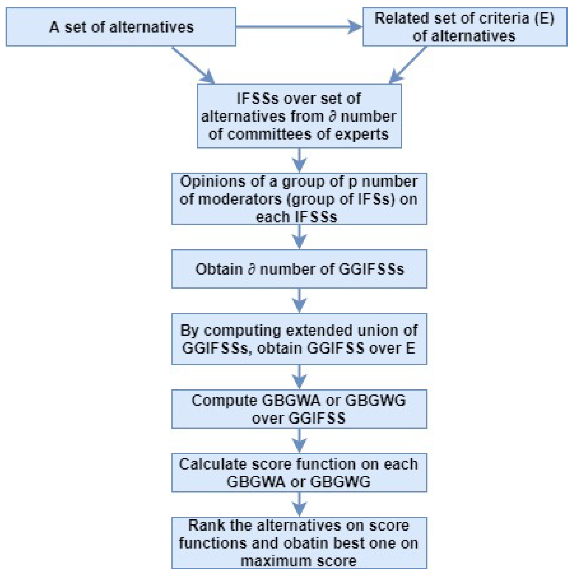
5. Multi-Attribute Decision Making under GGIFSSs Environment

In this section, firstly we present our approach comprising of an algorithm by virtue of GGIFSSs, and GBGWA or GBGWG operators. Then, we conduct two illustrations on proposed method as in the case studies: (1) candidates evaluation for an insurance company; and (2) cinema selection for the customers.

5.1. Proposed Method

As stated above, the properties of boundedness and monotonicity are valid for proposed operators. Therefore, a comparison can be made among two or more GBGWA(GBGWG) operators. Let $\varsigma$ be the number of committees established comprising specialists, which are intended to classify each alternative ${\kappa }_j(j=1,2,\dots ,n)$, while making in account with the imperative attributes ${\upsilon }_i(i=1,2,\dots ,m)$, and by provision of their respective grades in terms of IFSSs. Consider $d_1,d_2,\dots ,d_p$ be the members/experts(directors or officers), who are in-charge of constituted committees. Thereafter, the subjective information (in the form of IFSSs) from committees is collected. The senior experts will examine it and give their judgements as a group of IFSs. Then, the information of each committee comprised the GGIFSS, and there will be $\varsigma$ number of GGIFSSs. The extended union on GGIFSSs is computed, denoted as ${\tilde{\mathcal{G}}}_{\tilde{g}}$ and expressed in a table. Here, two types of criteria occur in the ${\tilde{\mathcal{G}}}_{\tilde{g}}$, namely, benefit and cost criteria. To consolidate the criteria, the ${\tilde{\mathcal{G}}}_{\tilde{g}}$ must be normalized through the following equation:

$$r_{ji}=\left\{\begin{array}{cc}\langle {\tilde{t}}_{\mathcal{A}}({\upsilon }_i),{\tilde{f}}_{\mathcal{A}}({\upsilon }_i)\rangle ,\hfill & \mathrm{if}{\upsilon }_i\mathrm{is}\mathrm{a}\mathrm{benefit}\mathrm{criterion},\hfill \\ \langle {\tilde{f}}_{\mathcal{A}}({\upsilon }_i),{\tilde{t}}_{\mathcal{A}}({\upsilon }_i)\rangle ,\hfill & \mathrm{if}{\upsilon }_i\mathrm{is}\mathrm{a}\cos \mathrm{t}\mathrm{criterion},\hfill \end{array}\right.$$

(10)

such that the normalized GGIFSS is denoted by ${\widetilde{{\mathcal{G}}^{\prime }}}_{\tilde{g}}=({\tilde{\mathcal{T}}}^{\prime },E,{\tilde{g}}^{\prime })$, where $({\tilde{\mathcal{T}}}^{\prime },E)$ is the normalization of $(\tilde{\mathcal{T}},E)$ and ${\tilde{g}}^{\prime }$ is the normalization of $\tilde{g}$. Finally, GBGWA or GBGWG can be used to aggregate the data from ${\widetilde{{\mathcal{G}}^{\prime }}}_{\tilde{g}}$ and each ${\ell }_j^{\prime }$ or ${\ell }_j^{\prime \prime }$ can be correlated through score function. Therefore, we propose our methodology as an algorithm as follows.

Algorithm 1 Multi-attribute decision making on GGIFSSs
Input: A set of alternatives
Output: The felicitous alternative for a problem
1:	Let $X=\{{\kappa }_1,{\kappa }_2,\dots ,{\kappa }_n\}$ be the set of alternatives and $E={\mathcal{A}}_1\cup {\mathcal{A}}_2\cup ,\dots ,\cup {\mathcal{A}}_{\varsigma }=\{{\upsilon }_1,{\upsilon }_2,\dots ,{\upsilon }_m\}$ be the set of attributes. Constitute a mechanism of the specialists’ judgements on attributes in the form of IFVs and establish IFSSs on each committee of specialists.
2:	Obtain $\varsigma$ number of GGIFSSs, ${\tilde{\mathcal{F}}}_{\tilde{g}1}=({\tilde{\mathcal{S}}}_1,{\mathcal{A}}_1,{\tilde{g}}_1)$, ${\tilde{\mathcal{F}}}_{\tilde{g}2}=({\tilde{\mathcal{S}}}_2,{\mathcal{A}}_2,{\tilde{g}}_2)$, …, ${\tilde{\mathcal{F}}}_{\tilde{g}\varsigma }=({\tilde{\mathcal{S}}}_{\varsigma },{\mathcal{A}}_{\varsigma },{\tilde{g}}_{\varsigma })$ over X, which are handled by $\varsigma$ number of committees of experts and specialists. Each group ${\tilde{g}}_1,{\tilde{g}}_2,\dots ,{\tilde{g}}_{\varsigma }$ of IFSs is constituted by p number of senior members/moderators for available information on each ${\mathcal{A}}_{i^{\prime }}(i^{\prime }=1,2,\dots ,\varsigma )$, respectively.
3:	Compute extended union ${\tilde{\mathcal{G}}}_{\tilde{g}}={({\tilde{\bigsqcup }}_{\mathcal{E}})}_{i^{\prime }=1}^{\varsigma }{\tilde{\mathcal{F}}}_{\tilde{g}{i}^{\prime }}$ of GGIFSSs. Represent ${\tilde{\mathcal{G}}}_{\tilde{g}}$ in a table.
4:	Normalized the data in ${\tilde{\mathcal{G}}}_{\tilde{g}}$ using Equation (3), and represent ${\widetilde{{\mathcal{G}}^{\prime }}}_{\tilde{g}}$ in a table.
5:	Calculate GBGWA ${\ell }_j^{\prime }(j=1,2,\dots ,n)$ or GBGWG ${\ell }_j^{″}(j=1,2,\dots ,n)$ operators on GGIFFS ${\widetilde{{\mathcal{G}}^{\prime }}}_{\tilde{g}}$. There will be n operators.
6:	Obtain score function on each operator ${\ell }_j^{\prime }$ or ${\ell }_j^{″}$ using Definition 3.
7:	Rank the alternatives on score function; the best choice is obtained on a maximum score.

This algorithm is depicted as a flowchart in Figure 1. The Algorithm 1 can be formulated to select the best product or alternative for p number of customers. In this way, the extra inputs incorporate as the demands of customers in GGIFSS, and the Algorithm 1 will conduct on a GGIFSS, ${\tilde{\mathcal{F}}}_{\tilde{g}}=(\tilde{\mathcal{S}},E,\tilde{g})$, from Step 4. To operate above methodology, we establish two case studies as below.

5.2. Case Study: Candidate Selection Problem

In this case study, an example for evaluation of candidates is used to illustrate the applicability of the proposed method. An insurance company HG in Guangzhou, China is engaged for insurance of products, charging insurance premium, consultation on insurance, financial and other services for individuals and enterprises. Every year, this company recruits new staff for the post of insurance sales agents and consultants. To maintain the excellence and high admire reputation, the company consults with experts for their assessments and opinions to recruit the candidates. Furthermore, the insurance business department and human resources department are actively engaged in recruitment process.

Let $X=\{{\kappa }_1,{\kappa }_2,{\kappa }_3,{\kappa }_4,{\kappa }_5\}$ be the set of five candidates whom can be placed for the position of insurance sales consultant. A group of three senior members (directors, officers, etc.) $d_1,d_2$ and $d_3$ setup a committee of specialists and experts to appoint a felicitous candidate for this position. The set of criteria for committee to select the candidate is $E=\{{\upsilon }_1,{\upsilon }_2,{\upsilon }_3,{\upsilon }_4,{\upsilon }_5,{\upsilon }_6,{\upsilon }_7\}$, where

• ${\upsilon }_1:$ english level;
• ${\upsilon }_2:$ relevant problem solving skills;
• ${\upsilon }_3:$ relevant working experience;
• ${\upsilon }_4:$ communication skills;
• ${\upsilon }_5:$ finance and insurance professional;
• ${\upsilon }_6:$ score obtained in a college degree; and
• ${\upsilon }_7:$ interpersonal skills.

On the set parameters, the weight vector is given and denoted by $w={(w_1/0.12,w_2/0.13,w_3/0.15,w_4/0.15,w_5/0.17,w_6/0.11,w_7/0.17)}^T$ such that ${\sum }_{i=1}^7{w}_i=1$. The three senior members arrange specialists into two groups; the first group consists of the specialists of insurance business management and the second group consists of the specialists of human resource management. The set of parameters $\mathcal{A}=\{{\upsilon }_2,{\upsilon }_3,{\upsilon }_5\}$ is assigned for first group and the set of parameters $\mathcal{B}=\{{\upsilon }_1,{\upsilon }_4,{\upsilon }_6,{\upsilon }_7\}$ is assigned for second group. These two groups give their judgments as IFSSs $({\tilde{\mathcal{S}}}_1,\mathcal{A})$ and $({\tilde{\mathcal{S}}}_2,\mathcal{B})$, respectively. Then, the group of senior members examine the data of IFSSs and then provide the two groups of IFSs, $g_1=\{{\tilde{\alpha }}_{d_1},{\tilde{\alpha }}_{d_2},{\tilde{\alpha }}_{d_3}\}$ and $g_2=\{{\tilde{\beta }}_{d_1},{\tilde{\beta }}_{d_2},{\tilde{\beta }}_{d_3}\}$ to complete the GGIFSSs, ${\tilde{\mathcal{F}}}_{\tilde{g}1}=({\tilde{\mathcal{S}}}_1,\mathcal{A},{\tilde{g}}_1)$ and ${\tilde{\mathcal{F}}}_{\tilde{g}2}=({\tilde{\mathcal{S}}}_2,\mathcal{B},{\tilde{g}}_2)$, as shown in

Table 5. Tabular representation of the GGIFSS ${\tilde{\mathcal{F}}}_{\tilde{g}1}=({\tilde{\mathcal{S}}}_1,\mathcal{A},{\tilde{g}}_1)$.

$\mathit{X}\setminus \mathcal{A}$	${\mathit{\upsilon }}_2$	${\mathit{\upsilon }}_3$	${\mathit{\upsilon }}_5$
${\kappa }_1$	$\langle 0.7,0.1\rangle$	$\langle 0.7,0.1\rangle$	$\langle 0.6,0.1\rangle$
${\kappa }_2$	$\langle 0.5,0.3\rangle$	$\langle 0.6,0.3\rangle$	$\langle 0.6,0.4\rangle$
${\kappa }_3$	$\langle 0.5,0.4\rangle$	$\langle 0.5,0.4\rangle$	$\langle 0.9,0.1\rangle$
${\kappa }_4$	$\langle 0.3,0.4\rangle$	$\langle 0.7,0.2\rangle$	$\langle 0.7,0.2\rangle$
${\kappa }_5$	$\langle 0.6,0.4\rangle$	$\langle 0.6,0.4\rangle$	$\langle 0.8,0.1\rangle$
${\tilde{\alpha }}_{d_1}$	$\langle 0.5,0.2\rangle$	$\langle 0.5,0.4\rangle$	$\langle 0.7,0.2\rangle$
${\tilde{\alpha }}_{d_2}$	$\langle 0.4,0.4\rangle$	$\langle 0.4,0.6\rangle$	$\langle 0.3,0.5\rangle$
${\tilde{\alpha }}_{d_3}$	$\langle 0.6,0.4\rangle$	$\langle 0.3,0.5\rangle$	$\langle 0.5,0.5\rangle$

and

Table 6. Tabular representation of the GGIFSS ${\tilde{\mathcal{F}}}_{\tilde{g}2}=({\tilde{\mathcal{S}}}_2,\mathcal{B},{\tilde{g}}_2)$.

$\mathit{X}\setminus \mathcal{B}$	${\mathit{\upsilon }}_1$	${\mathit{\upsilon }}_4$	${\mathit{\upsilon }}_6$	${\mathit{\upsilon }}_7$
${\kappa }_1$	$\langle 0.5,0.5\rangle$	$\langle 0.6,0.1\rangle$	$\langle 0.6,0.4\rangle$	$\langle 0.7,0.1\rangle$
${\kappa }_2$	$\langle 0.5,0.4\rangle$	$\langle 0.3,0.4\rangle$	$\langle 0.5,0.4\rangle$	$\langle 0.8,0.2\rangle$
${\kappa }_3$	$\langle 0.4,0.4\rangle$	$\langle 0.7,0.2\rangle$	$\langle 0.6,0.3\rangle$	$\langle 0.4,0.4\rangle$
${\kappa }_4$	$\langle 0.5,0.2\rangle$	$\langle 0.7,0.3\rangle$	$\langle 0.7,0.2\rangle$	$\langle 0.5,0.3\rangle$
${\kappa }_5$	$\langle 0.7,0.2\rangle$	$\langle 0.8,0.1\rangle$	$\langle 0.6,0.3\rangle$	$\langle 0.6,0.1\rangle$
${\tilde{\beta }}_{d_1}$	$\langle 0.4,0.3\rangle$	$\langle 0.7,0.3\rangle$	$\langle 0.6,0.2\rangle$	$\langle 0.7,0.2\rangle$
${\tilde{\beta }}_{d_2}$	$\langle 0.6,0.4\rangle$	$\langle 0.3,0.4\rangle$	$\langle 0.3,0.6\rangle$	$\langle 0.5,0.3\rangle$
${\tilde{\beta }}_{d_3}$	$\langle 0.5,0.5\rangle$	$\langle 0.4,0.5\rangle$	$\langle 0.4,0.4\rangle$	$\langle 0.7,0.2\rangle$

, respectively.

To evaluate most felicitous candidate on provided information in Table 5 and Table 6, the extended intersection of ${\tilde{\mathcal{F}}}_{\tilde{g}1}$ and ${\tilde{\mathcal{F}}}_{\tilde{g}2}$ is contemplated as follows:

$${\tilde{\mathcal{G}}}_{\tilde{g}}={\tilde{\mathcal{F}}}_{\tilde{g}1}{\tilde{\bigsqcup }}_{\mathcal{E}}{\tilde{\mathcal{F}}}_{\tilde{g}2}=(\tilde{\mathcal{T}},E,\tilde{g})=({\tilde{\mathcal{S}}}_1,\mathcal{A},{\tilde{g}}_1){\tilde{\bigsqcup }}_{\mathcal{E}}({\tilde{\mathcal{S}}}_2,\mathcal{B},{\tilde{g}}_2)$$

and shown in

Table 7. Tabular representation of the GGIFSS ${\tilde{\mathcal{F}}}_{\tilde{g}1}{\tilde{\bigsqcup }}_{\mathcal{E}.}{\tilde{\mathcal{F}}}_{\tilde{g}2}$.

$\mathit{X}\setminus \mathit{E}$	${\mathit{\upsilon }}_1$	${\mathit{\upsilon }}_2$	${\mathit{\upsilon }}_3$	${\mathit{\upsilon }}_4$	${\mathit{\upsilon }}_5$	${\mathit{\upsilon }}_6$	${\mathit{\upsilon }}_7$
${\kappa }_1$	$\langle 0.5,0.5\rangle$	$\langle 0.7,0.1\rangle$	$\langle 0.7,0.1\rangle$	$\langle 0.6,0.1\rangle$	$\langle 0.6,0.1\rangle$	$\langle 0.6,0.4\rangle$	$\langle 0.7,0.1\rangle$
${\kappa }_2$	$\langle 0.5,0.4\rangle$	$\langle 0.5,0.3\rangle$	$\langle 0.6,0.3\rangle$	$\langle 0.3,0.4\rangle$	$\langle 0.6,0.4\rangle$	$\langle 0.5,0.4\rangle$	$\langle 0.8,0.2\rangle$
${\kappa }_3$	$\langle 0.4,0.4\rangle$	$\langle 0.5,0.4\rangle$	$\langle 0.5,0.4\rangle$	$\langle 0.7,0.2\rangle$	$\langle 0.9,0.1\rangle$	$\langle 0.6,0.3\rangle$	$\langle 0.4,0.4\rangle$
${\kappa }_4$	$\langle 0.5,0.2\rangle$	$\langle 0.3,0.4\rangle$	$\langle 0.7,0.2\rangle$	$\langle 0.7,0.3\rangle$	$\langle 0.7,0.2\rangle$	$\langle 0.7,0.2\rangle$	$\langle 0.5,0.3\rangle$
${\kappa }_5$	$\langle 0.7,0.2\rangle$	$\langle 0.6,0.4\rangle$	$\langle 0.6,0.4\rangle$	$\langle 0.8,0.1\rangle$	$\langle 0.8,0.1\rangle$	$\langle 0.6,0.3\rangle$	$\langle 0.6,0.1\rangle$
${\tilde{\gamma }}_{d_1}$	$\langle 0.4,0.3\rangle$	$\langle 0.5,0.2\rangle$	$\langle 0.5,0.4\rangle$	$\langle 0.7,0.3\rangle$	$\langle 0.7,0.2\rangle$	$\langle 0.6,0.2\rangle$	$\langle 0.7,0.2\rangle$
${\tilde{\gamma }}_{d_2}$	$\langle 0.6,0.4\rangle$	$\langle 0.4,0.4\rangle$	$\langle 0.4,0.6\rangle$	$\langle 0.3,0.4\rangle$	$\langle 0.3,0.5\rangle$	$\langle 0.3,0.6\rangle$	$\langle 0.5,0.3\rangle$
${\tilde{\gamma }}_{d_3}$	$\langle 0.5,0.5\rangle$	$\langle 0.6,0.4\rangle$	$\langle 0.3,0.5\rangle$	$\langle 0.4,0.5\rangle$	$\langle 0.5,0.5\rangle$	$\langle 0.4,0.4\rangle$	$\langle 0.7,0.2\rangle$

.

As the all criterion are benefit type, the normalized GGIFSS, ${\tilde{\mathcal{G}}}_{\tilde{g}}$, is not needed. The weight vector for three senior members is given by $\varpi ={({\varpi }_1/0.33,{\varpi }_2/0.34,{\varpi }_3/0.33)}^T$ such that ${\sum }_{k=1}^3{\varpi }_k=1$. The GBGWA operator is used on integrated data in Table 7, and given as follows:

$${\ell }_1^{\prime }=\mathrm{GGWA}(c_{11},c_{12},\dots ,c_{17})={\mathrm{IFWA}}_k(\langle 0.390932,0.353894\rangle ,\langle 0.260704,0.518795\rangle ,\langle 0.325209,0.489552\rangle )=\langle 0.327079,0.448601\rangle$$

$${\ell }_2^{\prime }=\mathrm{GGWA}(c_{21},c_{22},\dots ,c_{27})={\mathrm{IFWA}}_k(\langle 0.355421,0.494395\rangle ,\langle 0.237022,0.623437\rangle ,\langle 0.295668,0.600553\rangle )=\langle 0.297119,0.570421\rangle$$

$${\ell }_3^{\prime }=\mathrm{GGWA}(c_{31},c_{32},\dots ,c_{37})={\mathrm{IFWA}}_k(\langle 0.390064,0.455207\rangle ,\langle 0.260125,0.594251\rangle ,\langle 0.324487,0.569593\rangle )=\langle 0.326346,0.536655\rangle$$

$${\ell }_4^{\prime }=\mathrm{GGWA}(c_{41},c_{42},\dots ,c_{47})={\mathrm{IFWA}}_k(\langle 0.374141,0.435074\rangle ,\langle 0.249507,0.579256\rangle ,\langle 0.311241,0.553687\rangle )=\langle 0.312904,0.519253\rangle$$

$${\ell }_5^{\prime }=\mathrm{GGWA}(c_{51},c_{52},\dots ,c_{57})={\mathrm{IFWA}}_k(\langle 0.422383,0.383619\rangle ,\langle 0.281678,0.540934\rangle ,\langle 0.351372,0.513036\rangle )=\langle 0.353679,0.474575\rangle$$

Now, the score functions are calculated on above five operators and given as in the following: $\delta ({\ell }_1^{\prime })=0.439239$, $\delta ({\ell }_2^{\prime })=0.363349$, $\delta ({\ell }_3^{\prime })=0.394845$, $\delta ({\ell }_4^{\prime })=0.396825$, and $\delta ({\ell }_5^{\prime })=0.439552$. The descending order is acquired as ${\kappa }_5>{\kappa }_1>{\kappa }_4>{\kappa }_3>{\kappa }_2$; thus, ${\kappa }_5$ is the felicitous candidate for the position because $\delta ({\ell }_5^{\prime })=0.439552$ is the maximum score.

Next, a case study in a different scenario is given as follows.

5.3. Case Study: Alternative Evaluation on Customer Demands

Nowadays, the markets possess immense competition for the quality of service, besides the demands of customers are increased and widened in the different prospects. The service industries are booming and upgrading by entertainment, catering, tourism, and auction. Indeed, there is a fierce competition among the service industries, but currently film industry is in the most competitive position as customers always classify and compare cinemas on different parameters, such as convenience, environment, quality of service, upcoming movies, and expenses.

Let $X=\{{\kappa }_1,{\kappa }_2,{\kappa }_3,{\kappa }_4\}$ be the set of four cinemas. The set of attributes $E=\{{\upsilon }_1,{\upsilon }_2,{\upsilon }_3,{\upsilon }_4,{\upsilon }_5\}$, where

• ${\upsilon }_1:$ quality of service;
• ${\upsilon }_2:$ quality of expected films;
• ${\upsilon }_3:$ environment in cinema;
• ${\upsilon }_4:$ price reasonability; and
• ${\upsilon }_5:$ convenience and luxuriousness.

A committee of experts and specialists from a cinema management organization give the judgment for cinemas on provided attributes as an IFSSs $(\tilde{\mathcal{S}},E)$ (

Table 8. Tabular representation of the IFSS, $(\tilde{\mathcal{S}},E)$.

$\mathit{X}\setminus \mathit{E}$	${\mathit{\upsilon }}_1$	${\mathit{\upsilon }}_2$	${\mathit{\upsilon }}_3$	${\mathit{\upsilon }}_4$	${\mathit{\upsilon }}_5$
${\kappa }_1$	$\langle 0.4,0.5\rangle$	$\langle 0.5,0.5\rangle$	$\langle 0.6,0.4\rangle$	$\langle 0.3,0.4\rangle$	$\langle 0.3,0.3\rangle$
${\kappa }_2$	$\langle 0.6,0.4\rangle$	$\langle 0.6,0.3\rangle$	$\langle 0.5,0.4\rangle$	$\langle 0.4,0.4\rangle$	$\langle 0.6,0.3\rangle$
${\kappa }_3$	$\langle 0.3,0.4\rangle$	$\langle 0.4,0.4\rangle$	$\langle 0.5,0.4\rangle$	$\langle 0.6,0.4\rangle$	$\langle 0.5,0.5\rangle$
${\kappa }_4$	$\langle 0.5,0.3\rangle$	$\langle 0.3,0.3\rangle$	$\langle 0.3,0.4\rangle$	$\langle 0.4,0.6\rangle$	$\langle 0.5,0.3\rangle$
${\kappa }_5$	$\langle 0.6,0.4\rangle$	$\langle 0.5,0.3\rangle$	$\langle 0.5,0.5\rangle$	$\langle 0.5,0.4\rangle$	$\langle 0.3,0.4\rangle$

).

Now, the two customers $d_1$ and $d_2$ desire to choose a most suitable cinema to watch movies; their demands comprise IFSs,

$${\tilde{\alpha }}_{d_1}=\{{\upsilon }_1/\langle 0.4,0.6\rangle ,{\upsilon }_2/\langle 0.5,0.3\rangle ,{\upsilon }_3/\langle 0.5,0.4\rangle ,{\upsilon }_4/\langle 0.4,0.6\rangle ,{\upsilon }_5/\langle 0.4,0.4\rangle \},$$

$${\tilde{\alpha }}_{d_2}=\{{\upsilon }_1/\langle 0.5,0.4\rangle ,{\upsilon }_2/\langle 0.4,0.5\rangle ,{\upsilon }_3/\langle 0.5,0.3\rangle ,{\upsilon }_4/\langle 0.5,0.4\rangle ,{\upsilon }_5/\langle 0.4,0.2\rangle \}.$$

The attribute ${\upsilon }_4$ belongs to cost criteria, therefore corresponding IFVs can be normalized using Equation (10). Let $\tilde{g}=\{{\tilde{\alpha }}_{d_1},{\tilde{\alpha }}_{d_2}\}$ and the normalization of $\tilde{g}$ is expressed as ${\tilde{g}}^{\prime }=\{{\tilde{\alpha }}_{d_1}^{\prime },{\tilde{\alpha }}_{d_2}^{\prime }\}.$ Thereafter, Table 8 can be normalized. Then, the information can be extended into GGIFSS ${\widetilde{{\mathcal{F}}^{\prime }}}_{\tilde{g}}=(\widetilde{{\mathcal{S}}^{\prime }},E,{\tilde{g}}^{\prime })$, and specified in

Table 9. Tabular representation of the GGIFSS, $(\widetilde{{\mathcal{S}}^{\prime }},E,{\tilde{g}}^{\prime })$.

$\mathit{X}\setminus \mathit{E}$	${\mathit{\upsilon }}_1$	${\mathit{\upsilon }}_2$	${\mathit{\upsilon }}_3$	${\mathit{\upsilon }}_4$	${\mathit{\upsilon }}_5$
${\kappa }_1$	$\langle 0.4,0.5\rangle$	$\langle 0.5,0.5\rangle$	$\langle 0.6,0.4\rangle$	$\langle 0.4,0.3\rangle$	$\langle 0.3,0.3\rangle$
${\kappa }_2$	$\langle 0.6,0.4\rangle$	$\langle 0.6,0.3\rangle$	$\langle 0.5,0.4\rangle$	$\langle 0.4,0.4\rangle$	$\langle 0.6,0.3\rangle$
${\kappa }_3$	$\langle 0.3,0.4\rangle$	$\langle 0.4,0.4\rangle$	$\langle 0.5,0.4\rangle$	$\langle 0.4,0.6\rangle$	$\langle 0.5,0.5\rangle$
${\kappa }_4$	$\langle 0.5,0.3\rangle$	$\langle 0.3,0.3\rangle$	$\langle 0.3,0.4\rangle$	$\langle 0.6,0.4\rangle$	$\langle 0.5,0.3\rangle$
${\kappa }_5$	$\langle 0.6,0.4\rangle$	$\langle 0.5,0.3\rangle$	$\langle 0.5,0.5\rangle$	$\langle 0.4,0.5\rangle$	$\langle 0.3,0.4\rangle$
${\tilde{\alpha }}_{d_1}$	$\langle 0.4,0.6\rangle$	$\langle 0.5,0.3\rangle$	$\langle 0.5,0.4\rangle$	$\langle 0.6,0.4\rangle$	$\langle 0.4,0.4\rangle$
${\tilde{\alpha }}_{d_2}$	$\langle 0.5,0.4\rangle$	$\langle 0.4,0.5\rangle$	$\langle 0.5,0.3\rangle$	$\langle 0.4,0.5\rangle$	$\langle 0.4,0.2\rangle$

.

Let $w={(w_1/0.18,w_2/0.19,w_3/0.21,w_4/0.22,w_5/0.2)}^T$ be the weight vector for attributes and $\varpi ={({\varpi }_1/0.52,{\varpi }_2/0.48)}^T$ be the weight vector for customers. The GBGWA operator is used on integrated data in Table 9, and given as follows:

$${\ell }_1^{\prime }=\mathrm{GGWA}(c_{11},c_{21},\dots ,c_{15})={\mathrm{IFWA}}_k(\langle 0.220934,0.635540\rangle ,\langle 0.199004,0.605904\rangle )=\langle 0.210483,0.621138\rangle$$

$${\ell }_2^{\prime }=\mathrm{GGWA}(c_{21},c_{22},\dots ,c_{52})={\mathrm{IFWA}}_k(\langle 0.265324,0.619281\rangle ,\langle 0.238988,0.588324\rangle )=\langle 0.252798,0.604223\rangle$$

$${\ell }_3^{\prime }=\mathrm{GGWA}(c_{31},c_{32},\dots ,c_{35})={\mathrm{IFWA}}_k(\langle 0.209414,0.678382\rangle ,\langle 0.188627,0.652231\rangle )=\langle 0.199503,0.665701\rangle$$

$${\ell }_4^{\prime }=\mathrm{GGWA}(c_{41},c_{42},\dots ,c_{45})={\mathrm{IFWA}}_k(\langle 0.223041,0.608588\rangle ,\langle 0.200901,0.576761\rangle )=\langle 0.212491,0.593098\rangle$$

$${\ell }_5^{\prime }=\mathrm{GGWA}(c_{51},c_{52},\dots ,c_{55})={\mathrm{IFWA}}_k(\langle 0.227867,0.654431\rangle ,\langle 0.205248,0.626332\rangle )=\langle 0.217091,0.640789\rangle$$

Now, the score functions are calculated on above five operators and given as in the following: $\delta ({\ell }_1^{\prime })=0.294672$, $\delta ({\ell }_2^{\prime })=0.324287$, $\delta ({\ell }_3^{\prime })=0.266901$, $\delta ({\ell }_4^{\prime })=0.309696$, and $\delta ({\ell }_5^{\prime })=0.288151$. One can check that ${\kappa }_2$ is the suitable cinema for both customers as $\delta ({\ell }_2^{\prime })=0.324287$ is the maximum score.

Now, based on our results, comparisons with other methods are given in next section.

6. Comparisons and Discussions

In this section, we compare our framework and results with existing methodologies. At first, we make a comparison of our method with the framework presented in [44]. Then, we discuss the advantages of proposed technique.

6.1. Comparisons with the Method of Garg

Garg et al. [44] defined geometric and averaging operators on the GGIFSSs and then provided an algorithm for decision making methodology. Let $X=\{{\kappa }_1,{\kappa }_2,\dots ,{\kappa }_{n^{\prime }}\}$ be the set of alternatives and $E=\{{\upsilon }_1,{\upsilon }_2,\dots ,{\upsilon }_{m^{\prime }}\}$ be the set of criteria. To evaluate ${\kappa }_j(j=1,\dots ,n^{\prime })$ as a optimal choice, IFSS on E are given and assessments of moderators are given as an IFSs $G_{\varrho }(e)$, where $G=({\varrho }_1,{\varrho }_2,\dots ,{\varrho }_p)$ and $G_{\varrho }(e)$ denotes the opinion of experts on the elements of X by virtue of IFSS on E. We recall the algorithm contemplated in [44] and given as follows:

Algorithm 2 Grag’s Algorithm for faculty appointment
1:	Make a framework of the specialists’ judgment related to each possible choice (alternatives) in the form IFVs and then construct their corresponding decision matrix ${\left[h\right]}^{n^{\prime }\times m^{\prime }}.$
2:	Get the generalization matrix ${\left[G_{\varrho }\right]}^{n^{\prime }\times 1}$ by using the perceptions of the senior members/experts’ committee on each ${\kappa }_j$ $(j=1,2,\dots ,n^{\prime })$.
3:	Construct the new matrix ${\left[h_G\right]}^{n^{\prime }\times (m^{\prime }+1)}$ by placing ${\left[G_{\varrho }\right]}^{n^{\prime }\times 1}$ in ${\left[h\right]}^{n^{\prime }\times m^{\prime }}$ with respect to ${\kappa }_j$ $(j=1,2,\dots ,n^{\prime })$.
4:	Apply operators with respect to ${\kappa }_j$, and the results are denoted by $r_j^{\prime },j=1,2,\dots ,n^{\prime }.$
5:	Rank the ${\kappa }_j(j=1,2,\dots ,n^{\prime })$ in descending order on their score values $r_j^{\prime }$ $(j=1,2,\dots ,n^{\prime })$.

Under the approach established in [44], we provide some key points and compare Algorithm 1, with Algorithm 2:

(i)

In Algorithm 2, the generalized parameter matrix is obtained by incorporating preferences of experts on alternatives. In other words, information from moderator on alternatives is given; nevertheless, extra input can be sighted as another information over IFSS, and both information types (IFSS and extra inputs) deal with alternatives. Conversely, in Algorithm 1, clear and well-defined GGIFSSs are taken into account by incorporating IFSS and IFSs.

(ii)

Operation of extended union is used in Algorithm 1 on two GGIFSSs, while, in Algorithm 2, there are some difficulties in defining an operation of extended union on two or more GGIFSSs.

(iii)

It seems that GGWA or GGWG operators in Algorithm 2 are applied contrarily on two different information types, however, in Algorithm 1, an integrated manner is adopted to compile results through GBGWA or GBGWG.

(iv)

In Algorithm 1, the generalized parameters can be applied as the demands of customers, and thus an integrated framework can be employed in industries. However, Algorithm 2 lacks creating such frameworks.

6.2. Comparisons with the Results of GIFSSs

The obtained results on the case studies in Section 5.2 and Section 5.3 are compared with the outcomes that are achieved on GIFSSs as given below.

(i)

As discussed earlier, GGIFSS with only single generalized parameter is known as GIFSS. Then, Algorithm 1 can be separated for each senior moderator/customer in the case studies in Section 5.2 and Section 5.3.

1. Using the Lemma 1 and Algorithm 1, we obtained the results separately for each senior experts/members in the case study in Section 5.2. If only Senior Member 1 is taken into account during selection process, then $\delta ({\ell }_1^{\prime })=0.5185$, $\delta ({\ell }_2^{\prime })=0.4305$, $\delta ({\ell }_3^{\prime })=0.4674$, $\delta ({\ell }_4^{\prime })=0.4695$, and $\delta ({\ell }_5^{\prime })=0.5194$. The descending order is acquired as ${\kappa }_5>{\kappa }_1>{\kappa }_4>{\kappa }_3>{\kappa }_2$; thus, ${\kappa }_5$ is the felicitous candidate for the position.

If only Senior Member 2 is taken into account during selection process in the case study in Section 5.2, then $\delta ({\ell }_1^{\prime })=0.3709$, $\delta ({\ell }_2^{\prime })=0.3068$, $\delta ({\ell }_3^{\prime })=0.3329$, $\delta ({\ell }_4^{\prime })=0.3351$, and $\delta ({\ell }_5^{\prime })=0.3704$. The descending order is acquired as ${\kappa }_1>{\kappa }_5>{\kappa }_3>{\kappa }_4>{\kappa }_2$; thus, ${\kappa }_1$ is the felicitous candidate for the position.

If only Senior Member 3 is taken into account during selection process in the case study in Section 5.2, then $\delta ({\ell }_1^{\prime })=0.4178$, $\delta ({\ell }_2^{\prime })=0.3475$, $\delta ({\ell }_3^{\prime })=0.3774$, $\delta ({\ell }_4^{\prime })=0.3788$, and $\delta ({\ell }_5^{\prime })=0.4192$. The descending order is acquired as ${\kappa }_5>{\kappa }_1>{\kappa }_4>{\kappa }_2>{\kappa }_3$; thus, ${\kappa }_1$ is the felicitous candidate for the position.

It can be observed from above discussion that ${\kappa }_5$ is the most suitable candidate as per individual opinions of Senior Members 1 and 3. Similarly, ${\kappa }_1$ is the most felicitous candidate on individual opinion of Senior Member 2, while ${\kappa }_5$ is on second place in descending order. Thus, in general, ${\kappa }_5$ is the most suitable candidate.

2. Using the Lemma 1 and Algorithm 1, we obtained the results separately for each customer for the case study in Section 5.3. If it is required to select cinema only for Customer 1, then $\delta ({\ell }_1^{\prime })=0.2927$, $\delta ({\ell }_2^{\prime })=0.3230$, $\delta ({\ell }_3^{\prime })=0.2655$, $\delta ({\ell }_4^{\prime })=0.3072$, and $\delta ({\ell }_5^{\prime })=0.2867$. The order is acquired as ${\kappa }_2>{\kappa }_4>{\kappa }_1>{\kappa }_5>{\kappa }_3$; thus, ${\kappa }_2$ is the best cinema for Customer 1.

If it is required to select cinema only for the Customer 2, then $\delta ({\ell }_1^{\prime })=0.2965$, $\delta ({\ell }_2^{\prime })=0.3253$, $\delta ({\ell }_3^{\prime })=0.2682$, $\delta ({\ell }_4^{\prime })=0.3121$, and $\delta ({\ell }_5^{\prime })=0.2894$. The order is acquired as ${\kappa }_2>{\kappa }_4>{\kappa }_1>{\kappa }_5>{\kappa }_3$; thus, ${\kappa }_2$ is the best cinema for Customer 2.

Thus, in general, ${\kappa }_2$ is the most suitable for both customers.

(ii)

Feng et al. [42] introduced a framework of decision makings on GIFSSs. We correlate proposed results with their method as below. We acquired the results separately for each customer for the case study in Section 5.3. If it is required to select cinema only for Customer 1, then $\delta (Z_J({\kappa }_1))=0.5344$, $\delta (Z_J({\kappa }_2))=0.5928$, $\delta (Z_J({\kappa }_3))=0.4857$, $\delta (Z_J({\kappa }_1))=0.5549$, and $\delta (Z_J({\kappa }_1))=0.5251$. The descending order acquired as ${\kappa }_2>{\kappa }_4>{\kappa }_1>{\kappa }_5>{\kappa }_3$; thus, ${\kappa }_2$ is the best cinema for Customer 1. If it is require to select cinema only for Customer 2, then $\delta (Z_J({\kappa }_1))=0.5311$, $\delta (Z_J({\kappa }_2))=0.5961$, $\delta (Z_J({\kappa }_3))=0.4894$, $\delta (Z_J({\kappa }_1))=0.5568$, and $\delta (Z_J({\kappa }_1))=0.5262$. The descending order acquired as ${\kappa }_2>{\kappa }_4>{\kappa }_1>{\kappa }_5>{\kappa }_3$; thus, ${\kappa }_2$ is the best cinema for Customer 2.

(iii)

A framework for the best concept selection in design process has been computed in [43], where GIFSSs are utilized to acquire integrated information on customers demands and design concepts. To meet their objectives, they introduced an algorithm, which we updated as follows:

Algorithm 3 Updated form of Algorithm in [43]
1:	The demands of p number of customers are represented as IFSs ${\tilde{\alpha }}_1,{\tilde{\alpha }}_2,\dots ,{\tilde{\alpha }}_p$.
2:	Represent IFSS $(\tilde{\mathcal{S}},E)$ over set of all possible choices X.
3:	Represent GIFSSs for each customer ${\tilde{\mathcal{F}}}_k=(\tilde{\mathcal{S}},E,{\tilde{\alpha }}_k)(k=1,\dots ,p)$.
4:	Compute $int-AND-product$ operation on ${\tilde{\mathcal{F}}}_1,{\tilde{\mathcal{F}}}_2,\dots ,{\tilde{\mathcal{F}}}_p$, obtain GIFSS $\tilde{\mathcal{F}}$ and show it in tabular form.
5:	Derive the utility fuzzy set ${\Delta }_{\tilde{\mathcal{F}}}$ from the GIFSS $\tilde{\mathcal{F}}$.
6:	Output ${\kappa }_{j^{\prime }}$ as the optimal decision if ${\Delta }_{\tilde{\mathcal{F}}}({\kappa }_{j^{\prime }})=max\{{\Delta }_{\tilde{\mathcal{F}}}({\kappa }_j)\mid {\kappa }_j\in X\}$.
7:	If $j^{\prime }$ has more than one values then any one of ${\kappa }_j$ may be chosen.

The case study in Section 5.3 can be contemplated through Algorithm 3. On this prospect, GGIFSS given in Table 9 can be separated into two GIFSSs. After adopting all steps of Algorithm 3, $\Delta ({\kappa }_1)=0.2252$, $\Delta ({\kappa }_2)=0.2678$, $\Delta ({\kappa }_3)=0.2112$, $\Delta ({\kappa }_4)=0.2419$, and $\Delta ({\kappa }_5)=0.2261$. The descending order is acquired as ${\kappa }_2>{\kappa }_4>{\kappa }_5>{\kappa }_1>{\kappa }_3$; thus, ${\kappa }_2$ is the best cinema for both customers.

The superiorities and advantages of our method are given in next section.

7. Superiority of Proposed Method

In this section, we give some counter-examples to show the superiority of proposed method over recent approaches [42,43,44].

Example 5.

Assume a decision making problem by letting the two alternatives ${\kappa }_1$ and ${\kappa }_2$, which have to be evaluated by the committee of specialists over set of parameters $E=\{{\upsilon }_1,{\upsilon }_2,{\upsilon }_3\}$. The committee of specialists provide the judgments in the form of IFSS, given in

Table 10. Tabular representation of the IFSS, $(\tilde{\mathcal{S}},E)$.

$\mathit{X}\setminus \mathit{E}$	${\mathit{\upsilon }}_1$	${\mathit{\upsilon }}_2$	${\mathit{\upsilon }}_{\mathbf{3}}$
${\kappa }_1$	$\langle 0.5,0.5\rangle$	$\langle 0.4,0.6\rangle$	$\langle 0.6,0.4\rangle$
${\kappa }_2$	$\langle 0.3,0.7\rangle$	$\langle 0.5,0.4\rangle$	$\langle 0.5,0.3\rangle$

;

Here, we apply the approach provided by Feng et al. [42], by letting an extra input $\tilde{\beta }=\{\langle 0.4,0.2\rangle ,\langle 0.5,0.3\rangle ,\langle 0.6,0.4\rangle \}$ of a moderator. Then, the GIFSS is consolidated as in

Table 11. Tabular representation of the IFSS, $(\tilde{\mathcal{S}},E,\tilde{\beta })$.

$\mathit{X}\setminus \mathit{E}$	${\mathit{\upsilon }}_1$	${\mathit{\upsilon }}_2$	${\mathit{\upsilon }}_3$
${\kappa }_1$	$\langle 0.5,0.5\rangle$	$\langle 0.4,0.6\rangle$	$\langle 0.6,0.4\rangle$
${\kappa }_2$	$\langle 0.3,0.7\rangle$	$\langle 0.5,0.4\rangle$	$\langle 0.5,0.3\rangle$
$\tilde{\beta }$	$\langle 0.4,0.2\rangle$	$\langle 0.6,0.4\rangle$	$\langle 0.5,0.3\rangle$

;

The score function on IFVs in $\tilde{\beta }$ are $0.6,0.6$, and $0.6$ and the weights are $0.33,0.33$, and $0.33$, respectively. It can be seen that, when we convert extra input into weights in initial stages of decision making, the importance of membership and non-membership diminish. Using the method of Feng et al. [42], we get $\delta (Z_J({\kappa }_1))=0.503>\delta (Z_J({\kappa }_2))=0.498$ such that ${\kappa }_1>{\kappa }_2.$ Let $w=\{w_1/0.32,w_2/0.33,w_3/0.35\}$ be the weighted vector over E. Then, by proposed method, $\delta ({\ell }_1^{\prime })=0.310<\delta ({\ell }_2^{\prime })=0.314$ such that ${\kappa }_1<{\kappa }_2.$ Therefore, the conversation of extra input into weighted vector in early process of decision making diminish the importance of membership and non-membership. Thus, proposed approach is better then the method of Feng et al. [42].

Example 6.

Assume that ${\kappa }_1$, ${\kappa }_2$ and ${\kappa }_3$ are three products and $E=\{{\upsilon }_1,{\upsilon }_2,{\upsilon }_3\}$ is the set of parameters. The dependencies of products on criteria are provided in IFSS $(\tilde{\mathcal{S}},E)$ and given in

Table 12. Tabular representation of the IFSS, $(\tilde{\mathcal{S}},E)$.

$\mathit{X}\setminus \mathit{E}$	${\mathit{\upsilon }}_1$	${\mathit{\upsilon }}_2$	${\mathit{\upsilon }}_3$
${\kappa }_1$	$\langle 0.3,0.5\rangle$	$\langle 0.5,0.3\rangle$	$\langle 0.6,0.2\rangle$
${\kappa }_2$	$\langle 0.2,0.6\rangle$	$\langle 0.3,0.4\rangle$	$\langle 0.6,0.4\rangle$
${\kappa }_3$	$\langle 0.4,0.4\rangle$	$\langle 0.4,0.3\rangle$	$\langle 0.5,0.3\rangle$

.

Here, we consider the methodology of Hayat et al. [43]. To select best product for two customers $d_1,d_2$, their demands are investigated as ${\tilde{\beta }}_{d_1}=\{\langle 0.3,0.5\rangle ,\langle 0.4,0.4\rangle ,\langle 0.6,0.2\rangle \}$, ${\tilde{\beta }}_{d_2}=\{\langle 0.3,0.6\rangle ,\langle 0.3,0.4\rangle ,\langle 0.5,0.4\rangle \}$, respectively. Then, the GIFSSs for $d_1$ and $d_2$ are given in

Table 13. GIFSS $(\tilde{\mathcal{S}},E,{\tilde{\beta }}_{d_1})$.

$\mathit{X}\setminus \mathit{E}$	${\mathit{\upsilon }}_1$	${\mathit{\upsilon }}_2$	${\mathit{\upsilon }}_3$
${\kappa }_1$	$\langle 0.3,0.5\rangle$	$\langle 0.5,0.3\rangle$	$\langle 0.6,0.2\rangle$
${\kappa }_2$	$\langle 0.2,0.6\rangle$	$\langle 0.3,0.4\rangle$	$\langle 0.6,0.4\rangle$
${\kappa }_3$	$\langle 0.4,0.4\rangle$	$\langle 0.4,0.3\rangle$	$\langle 0.5,0.3\rangle$
${\tilde{\beta }}_{d_1}$	$\langle 0.3,0.5\rangle$	$\langle 0.4,0.4\rangle$	$\langle 0.6,0.2\rangle$

and

Table 14. GIFSS $(\tilde{\mathcal{S}},E,{\tilde{\beta }}_{d_2})$.

$\mathit{X}\setminus \mathit{E}$	${\mathit{\upsilon }}_1$	${\mathit{\upsilon }}_2$	${\mathit{\upsilon }}_3$
${\kappa }_1$	$\langle 0.3,0.5\rangle$	$\langle 0.5,0.3\rangle$	$\langle 0.6,0.2\rangle$
${\kappa }_2$	$\langle 0.2,0.6\rangle$	$\langle 0.3,0.4\rangle$	$\langle 0.6,0.4\rangle$
${\kappa }_3$	$\langle 0.4,0.4\rangle$	$\langle 0.4,0.3\rangle$	$\langle 0.5,0.3\rangle$
${\tilde{\beta }}_{d_2}$	$\langle 0.3,0.6\rangle$	$\langle 0.3,0.4\rangle$	$\langle 0.5,0.4\rangle$

, respectively.

In [43], $AND$ operation is computed on two GIFSSs for product for two customers. One can check that

$$\tilde{\mathcal{S}}({\upsilon }_1)\wedge \tilde{\mathcal{S}}({\upsilon }_2)=\tilde{\mathcal{S}}({\upsilon }_1)\mathit{with}{\tilde{t}}_{{\tilde{\beta }}_{d_1}}({\upsilon }_1)\wedge {\tilde{t}}_{{\tilde{\beta }}_{d_2}}({\upsilon }_2)={\tilde{t}}_{{\tilde{\beta }}_{d_1}}({\upsilon }_1),{\tilde{f}}_{{\tilde{\beta }}_{d_1}}({\upsilon }_1)\vee {\tilde{f}}_{{\tilde{\beta }}_{d_2}}({\upsilon }_2)={\tilde{f}}_{{\tilde{\beta }}_{d_1}}({\upsilon }_1)$$

(11)

$$\tilde{\mathcal{S}}({\upsilon }_1)\wedge \tilde{\mathcal{S}}({\upsilon }_3)=\tilde{\mathcal{S}}({\upsilon }_1)\mathit{with}{\tilde{t}}_{{\tilde{\beta }}_{d_1}}({\upsilon }_1)\wedge {\tilde{t}}_{{\tilde{\beta }}_{d_2}}({\upsilon }_3)={\tilde{t}}_{{\tilde{\beta }}_{d_1}}({\upsilon }_1),{\tilde{f}}_{{\tilde{\beta }}_{d_1}}({\upsilon }_1)\vee {\tilde{f}}_{{\tilde{\beta }}_{d_2}}({\upsilon }_3)={\tilde{f}}_{{\tilde{\beta }}_{d_1}}({\upsilon }_1)$$

(12)

$$\tilde{\mathcal{S}}({\upsilon }_2)\wedge \tilde{\mathcal{S}}({\upsilon }_3)=\tilde{\mathcal{S}}({\upsilon }_2)\mathit{with}{\tilde{t}}_{{\tilde{\beta }}_{d_1}}({\upsilon }_2)\wedge {\tilde{t}}_{{\tilde{\beta }}_{d_2}}({\upsilon }_3)={\tilde{t}}_{{\tilde{\beta }}_{d_1}}({\upsilon }_2),{\tilde{f}}_{{\tilde{\beta }}_{d_1}}({\upsilon }_2)\vee {\tilde{f}}_{{\tilde{\beta }}_{d_2}}({\upsilon }_3)={\tilde{f}}_{{\tilde{\beta }}_{d_1}}({\upsilon }_2).$$

(13)

It can be seen that, using $AND$ operation, the importance of IFVs for ${\upsilon }_2$ and ${\upsilon }_3$ are diminished in Equations (11) and (12). The importance of IFVs for ${\upsilon }_3$ are diminished in Equation (13). Thus, such an approach is not valid in the initial stages of decision making; therefore, for this prospect, the proposed approach is better then Hayat et al. [43].

In [44], GWA is computed on two information; one from a committee of experts (in form of IFSS) and other from group of senior persons. The extra inputs can be seen as a so-called IFSS of a group of senior persons over alternatives. Consider Example 5, where IFSS from a committee of experts is given in Table 10. The extra input is given in

Table 15. Opinions of experts on alternatives.

$\mathit{X}\setminus \mathit{experts}$	${\mathit{d}}_1$	${\mathit{d}}_2$
${\kappa }_1$	$\langle 0.4,0.5\rangle$	$\langle 0.4,0.4\rangle$
${\kappa }_2$	$\langle 0.3,0.3\rangle$	$\langle 0.2,0.4\rangle$

, and can be seen as a so-called IFSS on alternatives. In the prospect of Garg et al. [44], the extra opinions of the two senior experts $d_1,d_2$ can be merged with IFSS in Table 10.

Clearly, the combination of two data ((i) IFSS and (ii) IFVs of experts) based matrix is analyzed as GGIFSS in [44]. In another way, if it might be recognized that the group of extra inputs of senior experts is a summarization of the data (IFSS obtained from a committee of specialists), then the results can be obtained from Table 15, thus why would we contemplate two data based matrix over alternatives? Nevertheless, there exist some serious difficulties in [44]. Noteworthily, the proposed results are superior in certain aspects and a well-defined manner is considered.

Advantages of Proposed Method

Based on correlative and comparative research, the following benefits of present framework are acquired and emphasized:

(i)

The case study indicated in [44] is implemented on two IFVs based matrix but not for the GGIFSSs. The extra inputs are located as in IFVs type weights on alternatives and operators presumed to be collected on the two different IFVs based data. In this prospect, the proposed approach is based on well-defined GGIFSSs.

(ii)

In [42], an extra input turns into the weighted vector in initial stages of decision making after calculation of score functions but it is not integrated with the information of experts to achieve better results. In the proposed method, extra inputs are taken into account in an accurate way using GBGWA or GBGWG.

(iii)

In [43], the $AND$ operation is used on several GIFSSs. In many cases, $AND$ or $OR$ operations on IFVs provide instantaneous results but do not give comprehensively aggregated results.

(iv)

The judgements/demands of senior prospectors/customers in GGIFSSs as managed with proposed operators are useful to rank the alternatives. The proposed framework can be correlated with the shortening of any number of existing senior prospectors/customers.

8. Conclusions

It has been noticed that the definition of GGIFSS, given by Garg et al. [44], did not provide supplementary information in a precise manner. Under this prospect, we have reformulated the existing definition of GGIFSS by establishing a novel notion of GGIFSS and related operation are also refined. We have aggregated GBGWA and GBGWG operators on GGIFSSs, which are employed to aggregate our techniques. Then, we formulated the framework of decision makings in an algorithm and two case studies have been handled by virtue of proposed methodology. We have given the advantages and comparison with existing techniques and correlated the results which are achieved on GIFSSs. The advantages of given framework are to contemplate the prospector‘s demands or expert‘s judgments in an incorporated way such that establishing more operators can be constituted the design concept evaluation mechanism on GGIFSSs. In this way, the results presented in this paper can be studied in several fields, such as electrical engineering, industrial designs, construction engineering, as estimation of risk factors in risk management is a complex tasks thus such problem can be considered.

References

1. Maji, P.K.; Biswas, R.; Roy, A.R. Fuzzy soft sets. J. Fuzzy Math. 2001, 9, 589–602. [Google Scholar]
2. Zadeh, L.A. Fuzzy Sets. Inf. Control 1965, 8, 338–353. [Google Scholar] [CrossRef]
3. Molodtsov, D. Soft set theory-first results. Comput. Math. Appl. 1999, 37, 19–31. [Google Scholar] [CrossRef]
4. Maji, P.K.; Biswas, R.; Roy, A.R. Soft set theory. Comput. Math. Appl. 2003, 45, 555–562. [Google Scholar] [CrossRef] [Green Version]
5. Ali, M.I.; Feng, F.; Liu, X.; Min, W.K.; Shabir, M. On some new operations in soft set theory. Comput. Math. Appl. 2009, 57, 1547–1553. [Google Scholar] [CrossRef] [Green Version]
6. Roy, A.R.; Maji, P.K. A fuzzy soft set theoretic approach to decision making problems. J. Comput. Appl. Math. 2007, 203, 412–418. [Google Scholar] [CrossRef]
7. Alcantud, J.C.R.; Mathew, T.J. Separable fuzzy soft sets and decision making with positive and negative attributes. Appl. Soft Comput. 2017, 59, 586–595. [Google Scholar] [CrossRef]
8. Alcantud, J.C.R.; Torra, V. Decomposition theorems and extension principles for hesitant fuzzy sets. Inf. Fusion 2018, 41, 48–56. [Google Scholar] [CrossRef]
9. Khameneh, A.Z.; Kılıçman, A. Parameter reduction of fuzzy soft sets: An adjustable approach based on the three-way decision. Int. J. Fuzzy Syst. 2018, 20, 928–942. [Google Scholar] [CrossRef]
10. Hassan, N.; Sayed, O.R.; Khalil, A.M.; Ghany, M.A. Fuzzy soft expert system in prediction of coronary artery disease. Int. J. Fuzzy Syst. 2017, 19, 1546–1559. [Google Scholar] [CrossRef]
11. Hayat, K.; Ali, M.I.; Cao, B.Y.; Karaaslan, F.; Qin, Z. Characterizations of certain types of type-2 soft graphs. Discrete Dyn. Nat. Soc. 2018, 2018, 8535703. [Google Scholar] [CrossRef]
12. Hayat, K.; Ali, M.I.; Cao, B.; Karaaslan, F. New results on type-2 soft sets. J. Math. Stat. 2018, 484, 47. [Google Scholar] [CrossRef]
13. Hayat, K.; Ali, M.I.; Cao, B.-Y.; Yang, X.-P. A new type-2 soft set: Type-2 soft graphs and their applications. Adv. Fuzzy Sys. 2017. [Google Scholar] [CrossRef]
14. Kumar, A.; Kumar, D.; Jarial, S.K. A hybrid clustering method based on improved artificial bee colony and fuzzy C-means algorithm. Int. J. Artif. Intell. 2017, 15, 24–44. [Google Scholar]
15. Liu, Y.; Qin, K.; Martınez, L. Improving decision making approaches based on fuzzy soft sets and rough soft sets. Appl. Soft Comput. 2018, 65, 320–332. [Google Scholar] [CrossRef]
16. Medina, J.; Ojeda-Aciego, M. Multi-adjoint t-concept lattices. Inf. Sci. 2010, 180, 712–725. [Google Scholar] [CrossRef]
17. Pozna, C.; Minculete, N.; Precup, R.E.; Koczy, L.T.; Ballagi, A. Signatures: Definitions, operators and applications to fuzzy modelling. Fuzzy Sets Syst. 2012, 201, 86–104. [Google Scholar] [CrossRef]
18. Qinrong, F.; Fenfen, W. A discernibility matrix approach to fuzzy soft sets based decision making problems. J. Intell. Fuzzy Syst. 2018, 22, 59–74. [Google Scholar]
19. Vildan, C.; Halis, A. A topological view on L-fuzzy soft sets: Connectedness degree. J. Intell. Fuzzy Syst. 2018, 34, 1975–1983. [Google Scholar]
20. Vimala, J.; Arockia, J.R.; Anusuya, I.V.S. A study on fuzzy soft cardinality in lattice ordered fuzzy soft group and its application in decision making problems. J. Intell. Fuzzy. Syst. 2018, 34, 1535–1542. [Google Scholar] [CrossRef]
21. Xiao, F. A hybrid fuzzy soft sets decision making method in medical diagnosis. IEEE Acess 2018, 6, 25300–25312. [Google Scholar] [CrossRef]
22. Beg, I.; Rashid, T.; Jamil, R.N. Human attitude analysis based on fuzzy soft differential equations with Bonferroni mean. Comput. Appl. Math. 2018, 37, 2632–2647. [Google Scholar] [CrossRef]
23. Ma, X.; Zhan, J.; Ali, M.I. Applications of a kind of novel Z-soft fuzzy rough ideals to hemirings. J. Intell. Fuzzy Syst. 2017, 32, 2071–2080. [Google Scholar] [CrossRef]
24. Sun, B.; Ma, W. Soft fuzzy rough sets and its application in decision making. Artif. Intell. Rev. 2014, 41, 67–80. [Google Scholar] [CrossRef]
25. Atanassov, K. Intuitionistic fuzzy sets. Fuzzy Sets Syst. 1986, 20, 87–96. [Google Scholar] [CrossRef]
26. Atanassov, K. Intuitionistic Fuzzy Sets, Theory, and Applications; Series in Fuzziness and Soft Computing; Phisica-Verlag: Heidelberg, Germany, 1999. [Google Scholar]
27. Xu, Z. Intuitionistic fuzzy aggregation operators. IEEE Trans. Fuzzy Syst. 2007, 15, 1179–1187. [Google Scholar]
28. Xu, Z.; Yager, R.R. Some geometric aggregation operators based on intuitionistic fuzzy sets. Int. J. Gen. Syst. 2006, 35, 417–433. [Google Scholar] [CrossRef]
29. Jemal, H.; Kechaou, Z.; Ayed, M.B. Enhanced decision support systems in intensive care unit based on intuitionistic fuzzy sets. Adv. Fuzzy Syst. 2017, 2017, 7371634. [Google Scholar] [CrossRef]
30. Mukherjee, S. Selection of alternative fuels for sustainable urban transportation under multi-criteria intuitionistic fuzzy environment. Fuzzy Inf. Eng. 2017, 9, 117–135. [Google Scholar] [CrossRef]
31. Ren, H.P.; Chen, H.H.; Fei, W.; Li, D.F. A MAGDM method considering the amount and reliability information of interval-valued intuitionistic fuzzy sets. Int. J. Fuzzy Syst. 2017, 19, 15–25. [Google Scholar] [CrossRef]
32. Yun, S.M.; Lee, S.J. Intuitionistic fuzzy topologies induced by intuitionistic fuzzy approximation spaces. Int. J. Fuzzy Syst. 2017, 9, 285–291. [Google Scholar] [CrossRef]
33. Maji, P.K.; Biswas, R.; Roy, A.R. Intuitionistic fuzzy soft sets. J. Fuzzy Math. 2001, 9, 677–692. [Google Scholar]
34. Deli, I.; Karataş, S. Interval valued intuitionistic fuzzy parameterized soft set theory and its decision making. J. Intell. Fuzzy Syst. 2016, 30, 2073–2082. [Google Scholar] [CrossRef]
35. Akram, M.; Shahzadi, S. Novel intuitionistic fuzzy soft multiple-attribute decision-making methods. Neural Comput. Appl. 2018, 29, 435–447. [Google Scholar] [CrossRef]
36. Garg, H.; Arora, R. A nonlinear-programming methodology for multi-attribute decision-making problem with interval-valued intuitionistic fuzzy soft sets information. Appl. Intell. 2018, 48, 2031–2046. [Google Scholar] [CrossRef]
37. Garg, H.; Arora, R. Bonferroni mean aggregation operators under intuitionistic fuzzy soft set environment and their applications to decision-making. J. Oper. Res. Soc. 2018, 1–4. [Google Scholar] [CrossRef]
38. Garg, H.; Arora, R. Novel scaled prioritized intuitionistic fuzzy soft interaction averaging aggregation operators and their application to multi criteria decision making. Eng. Appl. Artif. Intell. 2018, 71, 100–112. [Google Scholar] [CrossRef]
39. Agarwal, M.; Biswas, K.K.; Hanmandlu, M. Generalized intuitionistic fuzzy soft sets with applications in decision-making. Appl. Soft Comput. 2013, 13, 3552–3566. [Google Scholar] [CrossRef]
40. Khalil, A.M. Commentary on Generalized intuitionistic fuzzy soft sets with applications in decision-making. Appl. Soft Comput. 2015, 37, 519–520. [Google Scholar] [CrossRef]
41. Yang, Y.; Wang, Y.; Zhang, Y.; Zhang, D. Commentary on generalized intuitionistic fuzzy soft sets with applications in decision-making [Appl. Soft Comput. 37 (2015) 519–520]. Appl. Soft Comput. 2016, 40, 427–428. [Google Scholar] [CrossRef]
42. Feng, F.; Fujita, H.; Ali, M.I.; Yager, R.R.; Liu, X. Another View on generalized Intuitionistic Fuzzy Soft Sets and Related Multiattribute Decision Making Methods. IEEE Trans. Fuzzy Syst. 2018. [Google Scholar] [CrossRef]
43. Hayat, K.; Ali, M.I.; Alcantud, J.C.R.; Cao, B.Y.; Tariq, K.U. Best concept selection in design process: An application of generalized intuitionistic fuzzy soft sets. J. Intell. Fuzzy Syst. 2018. [Google Scholar] [CrossRef]
44. Garg, H.; Arora, R. Generalized and group-based generalized intuitionistic fuzzy soft sets with applications in decision-making. Appl. Intell. 2018, 48, 343–356. [Google Scholar] [CrossRef]
45. Selvachandran, G.; Maji, P.K.; Faisal, R.Q.; Salleh, A.R. Distance and distance induced intuitionistic entropy of generalized intuitionistic fuzzy soft sets. Appl. Intell. 2017, 47, 132–147. [Google Scholar] [CrossRef]
46. Pawlak, Z. Rough sets. Int. J. Comput. Inf. Sci. 1982, 11, 341–356. [Google Scholar] [CrossRef]
47. Deschrijver, G.; Kerre, E. On the relationship between some extensions of fuzzy set theory. Fuzzy Sets Syst. 2003, 133, 227–235. [Google Scholar] [CrossRef]
48. Chen, S.M.; Tan, J.M. Handling multicriteria fuzzy decision-making problems based on vague set theory. Fuzzy Sets Syst. 1994, 67, 163–172. [Google Scholar] [CrossRef]
Figure 1. A flowchart for our algorithm.
Symmetry 10 00753 g001