Fuzzy Attribute Expansion Method for Multiple Attribute Decision-Making with Partial Attribute Values and Weights Unknown and Its Applications

Abstract

In the real world, there commonly exists types of multiple attribute decision-making (MADM) problems with partial attribute values and weights totally unknown. Symmetry among some attribute information that is already known and unknown, and symmetry between the pure attribute set and fuzzy attribute membership set can be a considerable way to solve this type of MADM problem. In this paper, a fuzzy attribute expansion method is proposed to solve this type of problem based on two key techniques: the spline interpolation technique and the attribute weight reconfiguration technique, which are respectively used for the determination of attribute values and the reconfiguration of attribute weights. The spline interpolation technique to expand attribute values can enhance the performance of some regression methods and clustering methods by the comparisons between the results of these methods dealing with practical cases with and without the application of the technique, which further illustrates the effectiveness of this technique. For MADM problems with partial attribute values and weights totally unknown, compared with traditional fuzzy comprehensive evaluation (FCE), FCE with the application of fuzzy attribute expansion method can obtain results more similar with the ones when all attribute values and weights are known, which is proved by the practical power quality evaluation example.

1. Introduction

Since fuzzy set was proposed by Zadeh [1] in 1965, fuzzy theory is used to quantitatively depict the fuzziness of processes or attributes of things, especially for multiple attribute decision-making (MADM) in some real-life problems.

The applications of fuzzy theory and related techniques in the MADM area can be basically classified into two categories: (1) Applications based on modifications of fuzzy set theory and its extension theories. Fuzzy comprehensive evaluation (FCE) is one of the most classic applications of fuzzy set theory to MADM. One-level FCE can effectively deal with an evaluation problem with a small number of evaluation index parameters (also called attributes). Zhao [2] proposed an electrocardiogram signal quality evaluation method based on one-level FCE and simple heuristic fusion. Yang [3] proposed a method to evaluate exposure, sensitivity, and adaptive capacity based on one-level FCE for better flood vulnerability assessment. Multi-level FCE is preferred as the number of attributes is large. To map porphyry-copper prospectivity in the Gangdese district, Tibet, western China, Zuo [4] established a two-level binary geoscience FCE including favorable rocks, intrusive rocks, faults, and geochemical anomalies. Besides, FCE also has been successfully applied to other MADM problems, e.g., image analysis [5,6], risk assessment [7,8], energy management [9,10], personnel selection [11], etc. As a successful extension of fuzzy set, intuitionistic fuzzy set (IFS) was initiated by Atanassov [12]. IFS uses membership degree, non-membership degree, and hesitancy degree to deal with fuzziness and uncertainty information, which is very useful for the resolution of MADM problems with incomplete attribute weights and uncertain attribute information [13,14,15,16,17]. Xu [13] proposed the models for MADM with intuitionistic fuzzy information based on IFS theory. Wan [14] proposed a new risk attitudinal method for IFS and applied it to the MADM of the teacher selection problem. Furthermore, with the initiation of interval-valued intuitionistic fuzzy set (IVIFS) by Atanassov [18], MADM based on IVIFS becomes a hot topic for researchers [19,20,21,22,23,24,25,26,27]. The applications of type-2 fuzzy sets [28,29,30], hesitant fuzzy sets [31,32], and dual hesitant fuzzy linguistic term sets [33] were also reported recently. From these applications, we can find that the extension theories provided researchers with more and more profound theoretical models of fuzzy theory to depict and solve the complicated real-life MADM problems. (2) Applications based on the combination between fuzzy theory and other MADM methods. There are about 20 MADM methods in the literature [34]. The analytic hierarchy process (AHP) [35,36] and technique for order of preference by similarity to ideal solution (TOPSIS) [37,38,39] are two of the most popular methods combined with fuzzy theory in the area of supplier evaluation [40]. These applications are based on the methodology that one MADM method can be modified by the combination of the other MADM methods. It could be useful in most cases, but the disadvantage is that an increase in computational complexity is also obvious, which is rarely discussed by researchers.

The applications mentioned above focus on the representation and calculation of fuzziness and uncertainty of attributes in MADM problems, the attribute information of which is completely given. As the deepening of understanding of MADM problems grows, researchers began to study MADM problems with incomplete attribute information in recent years. Here, we call such property of attribute information as the incompleteness of attribute, which has two forms, i.e., incomplete weights or values of partial attributes. For the type of problems with incomplete attribute weights information, Park [41] provided mathematical tools for interactive MADM from the perspective of pairwise dominance. Xu [42] determined the attribute weights by the optimization model based on the maximizing deviation method. Wei [43] proposed a gray relationship analysis method to calculate the weights for IFS. Bao [44] proposed an intuitionistic fuzzy decision method based on prospect theory and the evidential reasoning approach. For the type of problems with incomplete attribute values and weights, Eum [45] established dominance and potential optimality to evaluate whether the alternative outperforms for a fixed feasible region denoted by the constraints. There also exists the third type of MADM problems with some partial attribute values and weights totally unknown, i.e., no constraints of incomplete attributes, which is the extreme type of the above two types of problem. Actually, this type of problem is common in the real world, e.g., decision maker could not provide some attribute values and weights because of discreet principles or cognitive impairment, or some attribute values could not be obtained because of the failure of the data acquisition system, or there exists some unclear or undefined attributes of new things or processes. Thus, it is necessary to study and find out a solution to these type of MADM problems.

In the real world, attributes are partially correlated and continuous in the attribute space. Hence, if the fuzzy mapping is linear, the fuzzy values and weights of these attributes are also continuous, which means that for the correlated attributes of things or processes, fuzzy values and weights of some unknown attributes can be approximately estimated by the ones of some known attributes. Thus, based on the above new cognition of the mapping relationship between the objective world and fuzzy attribute set, we propose a fuzzy attribute expansion method, which consisted of the spline interpolation technique and attribute weight reconfiguration technique, to deal with the MADM problems with some partial attribute values and weights totally unknown.

The rest of the paper is organized as follows: Section 2 provides some basic definitions about the fuzzy set and some related sets. In Section 3, the formulaic expression of the third type of MADM problem is given based on the definitions in Section 2. The geometric analysis of the pure attribute set (PAS), the measurable attribute set (MAS), and the fuzzy attribute membership set (FAMS) of the problem is conducted in Section 4, which is the theoretic basis of the fuzzy attribute expansion method proposed in Section 5. Applications in regression, clustering, and power quality evaluation are presented in Section 6. In Section 7, the conclusions of the paper are given.

2. Basic Definitions

In this section, some basic concepts related to the method proposed in this paper are introduced and defined.

Definition 1.

([1]) A fuzzy set A in the universe of discourse $X=\left\{x_1,x_2,\cdots ,x_n\right\}$ is defined as follows:

$$A=\left\{\langle x,{\mu }_A\left(x\right)\rangle |x\in X\right\},$$

(1)

where ${\mu }_A\left(x\right):X\to \left[0,1\right]$ is the membership function.

Definition 2.

Assume that$x$has m kind of striking attributes (denoted as${\mathit{a}}_j^x\left(j=1,\cdots ,m\right)$), if a set$U_{\mathrm{p}}^x$of$x$ satisfying the following conditions:

(a) 

$\forall {\mathit{a}}_j^x\left(j=1,\cdots ,m\right)\in U_{\mathrm{p}}^x$

(b) 

${\mathit{a}}_i^x\propto {\mathit{a}}_j^x\left(i\ne j\right)$,

(c) 

${\mathit{a}}_i^x\cong h_i\left({\mathit{a}}_1^x,\cdots ,{\mathit{a}}_{i-1}^x,{\mathit{a}}_{i+1}^x\cdots ,{\mathit{a}}_m^x\right)$,

where $h_i$ is relationship function, then $U_{\mathrm{p}}^x$ is defined as the pure attribute set (PAS) of $x$.

If t$\left(t\ll m\right)$kind of attributes of$x$are only known, then define these t kind of attributes as knowable fuzzy attributes (KFA) and the other$\left(m-t\right)$kind of attributes as unknowable fuzzy attributes (UFA).

Definition 3.

If a set$U_{\mathrm{m}}^x$of$x$satisfying the following conditions:

(a) 

$\forall {\mathit{a}}_j^x\left(j=1,\cdots ,m\right)\in U_{\mathrm{p}}^x$,

(b) 

$\forall a_j^x=o_j\left({\mathit{a}}_j^x\right)\left(j=1,\cdots ,m\right)\in U_{\mathrm{m}}^x$,$o_j\left({\mathit{a}}_j^x\right):{\mathit{a}}_j^x\to {\mathrm{R}}^{1\times 1}$,

where$o_j$is an unknown function to measure the attribute$j$in the real world,$a_j^x$is the projection of attribute vector${\mathit{a}}_j^x$in some kind of space and expressed in numerical form, then$U_{\mathrm{m}}^x$is defined as the measurable attribute set (MAS) of$x$.

Definition 4.

If a set$U_{\mathrm{f}}^x$of$x$satisfying the following conditions:

(a) 

$\forall {\mathit{a}}_j^x\left(j=1,\cdots ,m\right)\in U_{\mathrm{p}}^x$,

(b) 

$\forall a_j^x=o_j\left({\mathit{a}}_j^x\right)\left(j=1,\cdots ,m\right)\in U_{\mathrm{m}}^x$,

(c) 

$\forall {\tilde{a}}_j^x={\nu }_j\left(a_j^x\right)\left(j=1,\cdots ,m\right)\in U_{\mathrm{f}}^x$,${\nu }_j\left(a_j^x\right):a_j^x\to \left[0,1\right]$,

where${\nu }_j\left(a_j^x\right):a_j^x\to \left[0,1\right]$is the attribute membership function,${\tilde{a}}_j^x$is fuzzy membership grade for attribute$j$of$x$, then$U_{\mathrm{f}}^x$is defined as the fuzzy attribute membership set (FAMS) of$x$.

For example, if${\mathit{a}}_j^x$is the volume attribute of a box,$a_j^x$could be the length of the box and the length unit is meter,$v_j$is the length attribute membership of satisfaction for customer, then${\tilde{a}}_j^x$is the fuzzy membership grade of length of the box.

3. Problem

In this section, some further definitions are defined based on the following theorems. Then, the main problem this paper focuses on is raised and expressed by these definitions.

Theorem 1.

PAS and FAMS of$x$are equivalent:$\mathrm{PAS}~\mathrm{FAMS}$.

Proof. 

$\because$$\forall {\tilde{a}}_j^x={\nu }_j\left(a_j^x\right)\left(j=1,\cdots ,m\right)$, $\forall a_j^x=o_j\left({\mathit{a}}_j^x\right)\left(j=1,\cdots ,m\right)$. $\therefore$$\forall {\tilde{a}}_j^x=v_j\left(o_j\left({\mathit{a}}_j^x\right)\right)\left(j=1,\cdots ,m\right)$, which means there exists one-to-one correspondence (bijection) from PAS to FAMS. Besides, $\left|\mathrm{PAS}\right|=\left|\mathrm{FAMS}\right|=m$. Thus, $\mathrm{PAS}~\mathrm{FAMS}$ is proved. □

Theorem 2.

PAS and FAMS of$x$are countable sets.

Proof. 

Choose random two attributes from FAMS of $x$ and denote them as ${\tilde{a}}_1^x$ and ${\tilde{a}}_m^x$, the other attributes are ranked by the similarity with ${\tilde{a}}_1^x$ and ${\tilde{a}}_m^x$ from large to small and inserted between ${\tilde{a}}_1^x$ and ${\tilde{a}}_m^x$, which comes out as the sequence

$${\tilde{S}}^x=\langle {\tilde{a}}_1^x,{\tilde{a}}_2^x,\cdots ,{\tilde{a}}_m^x\rangle .$$

By this method to rank PAS of $x$, it also comes out as the sequence

$${\mathit{S}}^x=\langle {\mathit{a}}_1^x,{\mathit{a}}_2^x,\cdots ,{\mathit{a}}_m^x\rangle .$$

Thus, PAS and FAMS of $x$ are both countable sets. □

Definition 5.

Based on Theorem 2, the attribute vector sequence of$x$is defined as follows:

$${\mathit{S}}^x=\langle {\mathit{a}}_1^x,{\mathit{a}}_2^x,\cdots ,{\mathit{a}}_m^x\rangle .$$

(2)

The measurable attribute sequence is defined as:

$$\begin{array}{ll}{S}^x& =\langle a_1^x,a_2^x,\cdots ,a_m^x\rangle \\ & =\underset{S_{\mathrm{KFA}}^x}{\underbrace{\langle a_{i-1}^x,\cdots ,a_{j-1}^x,\cdots ,a_{k-1}^x\rangle }}+\underset{S_{\mathrm{UFA}}^x}{\underbrace{\langle a_i^x,\cdots ,a_j^x,\cdots ,a_k^x\rangle }}\end{array}.$$

(3)

The fuzzy measurable attribute sequence of$x$has the following form:

$$\begin{array}{ll}{\tilde{S}}^x& =\langle {\tilde{a}}_1^x,{\tilde{a}}_2^x,\cdots ,{\tilde{a}}_m^x\rangle \\ & =\underset{{\tilde{S}}_{\mathrm{KFA}}^x}{\underbrace{\langle {\tilde{a}}_{i-1}^x,\cdots ,{\tilde{a}}_{j-1}^x,\cdots ,{\tilde{a}}_{k-1}^x\rangle }}+\underset{{\tilde{S}}_{\mathrm{UFA}}^x}{\underbrace{\langle {\tilde{a}}_i^x,\cdots ,{\tilde{a}}_j^x,\cdots ,{\tilde{a}}_k^x\rangle }}\end{array}.$$

(4)

Definition 6.

It is affirmative that KFA and UFA are correlated:

$${\tilde{S}}_{\mathrm{UFA}}^x\propto {\tilde{S}}_{\mathrm{KFA}}^x,$$

consider the function relations among these attributes is undefined:

$${\tilde{a}}_{j-1}^x=f\left({\tilde{a}}_j^x\right),$$

where function$f$has no exact analytic expression, so UFA can only be depicted by approximate estimation:

$${\widehat{\tilde{S}}}_{\mathrm{UFA}}^x\cong g\left({\tilde{S}}_{\mathrm{KFA}}^x\right),$$

where function$g$is the function for approximately estimating${\tilde{S}}_{\mathrm{UFA}}^x$with${\tilde{S}}_{\mathrm{KFA}}^x$ as the independent variable.

Based on the above definitions, the main problem this paper focused on can be described as follows:

Problem description: Given a set of fuzzy membership grades of KFA:

$$\left\{\langle i,{\tilde{S}}_{\mathrm{KFA}}^{x_i}\rangle |x_i\in X,i=1,\cdots ,n\right\},$$

evaluate $x_i$ under the following conditions:

(a)

The length of ${\tilde{S}}_{\mathrm{KFA}}^{x_i}$ is $t$, $t\ll m$;

(b)

The sequence of attribute weights is $\lambda =\langle {\lambda }_1,{\lambda }_2,\cdots ,{\lambda }_t\rangle$;

(c)

Evaluation value of $x_i$ falls into the interval $\left[0,1\right]$, the greater the evaluation value is, the higher the evaluation is.

(d)

The evaluation values are as similar to those obtained under the condition that some UFAs are given as possible.

Research about the problem with all conditions as mentioned above is rarely conducted. In fact, the condition (d) is an important index to evaluation. To satisfy condition (d), we suggest a fuzzy attribute expansion method to evaluate $x_i$: before the final evaluation, use KFAs to approximately estimate UFAs.

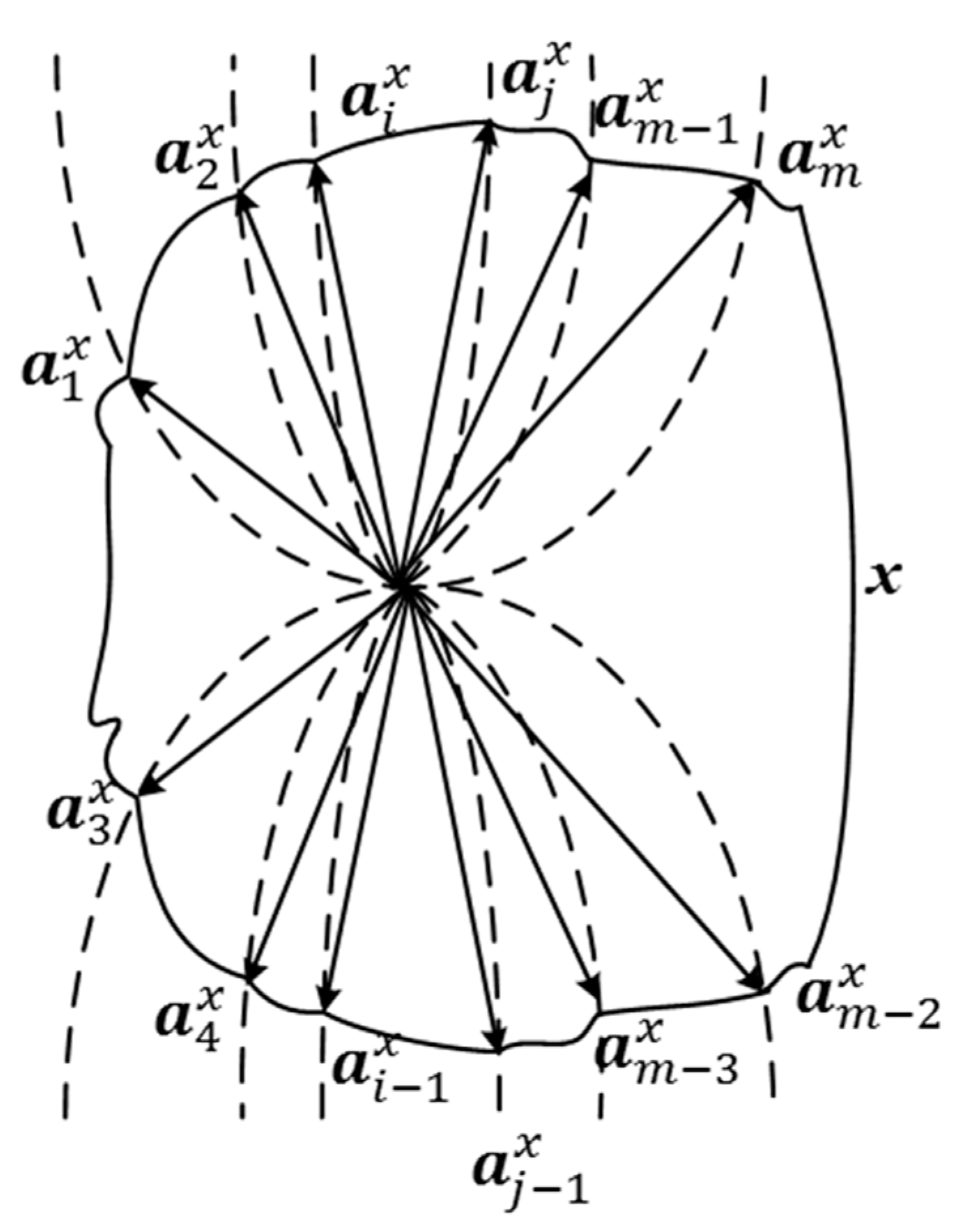
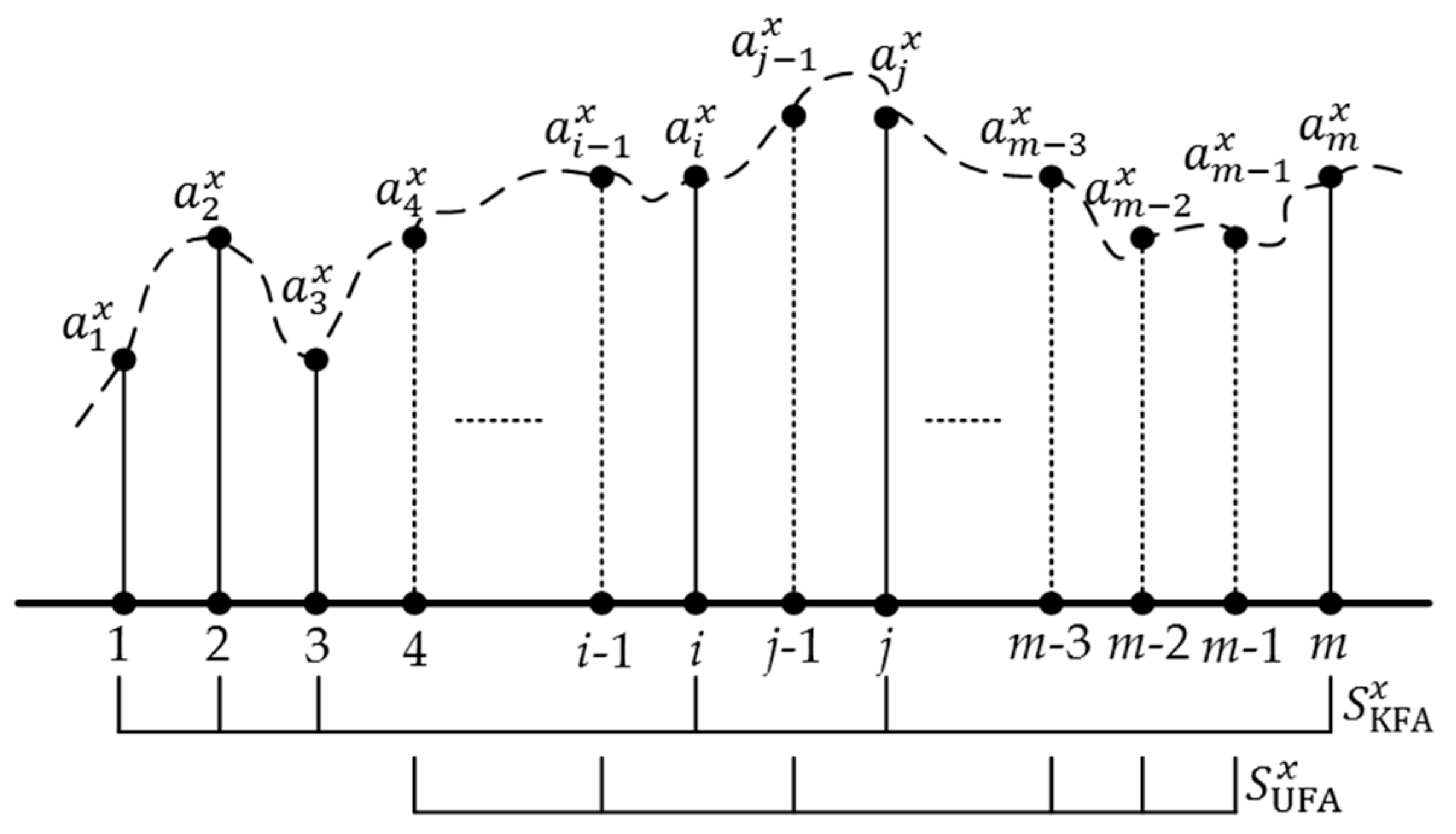
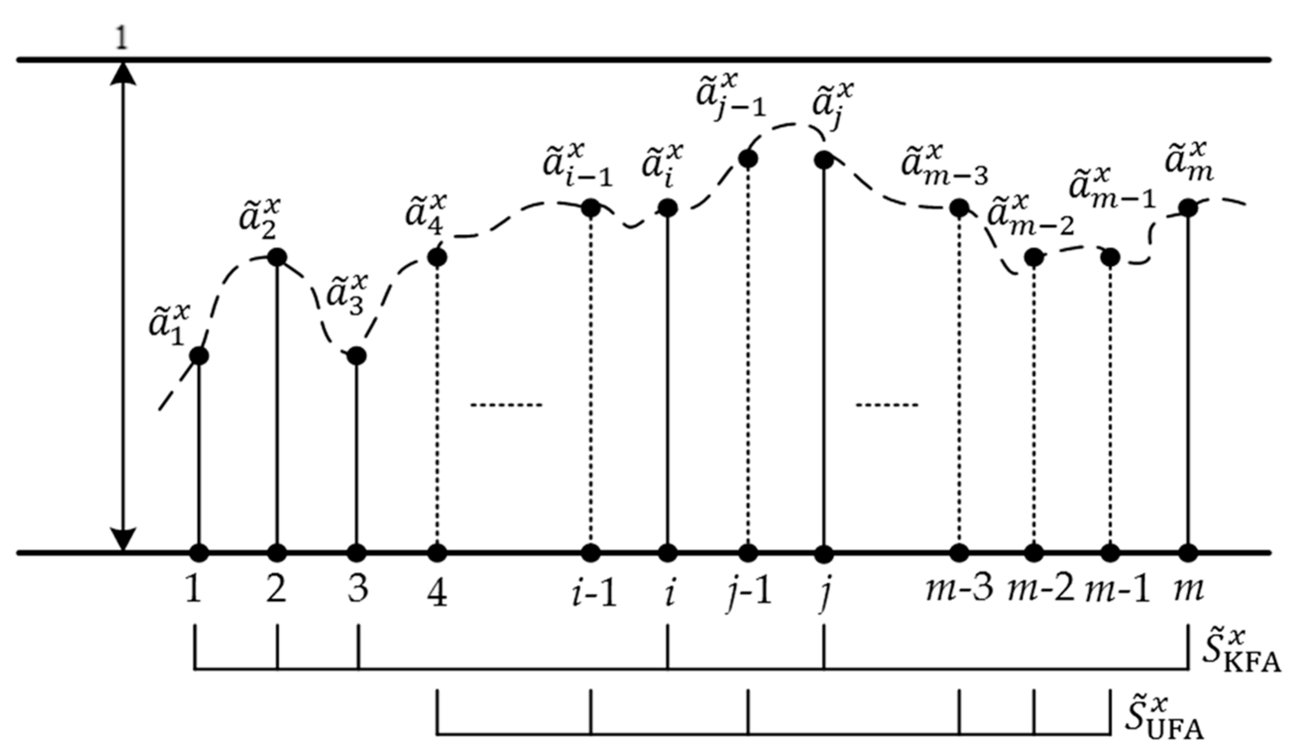
4. Geometric Analysis of PAS, MAS, and FAMS

In this section, the geometric analysis of PAS, MAS, and FAMS of the problem is conducted. Firstly, the generalized geometric structures (GGS) of PAS, MAS, and FAMS are modeled and represented in the form of a diagrammatic sketch. Secondly, the geometric relationship between GGS of PAS and GGS of FAMS is analyzed. Thirdly, GGS of $x$ in FAMS can be approximately estimated by the ${\tilde{S}}_{\mathrm{KFA}}^x$ of $x$ based on interpolation technique is discussed.

These three kinds of sets depict attributes, the relationships between attributes, and attribute membership degrees from different spatial cognition. PAS is an abstract set to characterize nonlinear relationships between attributes, especially the vague attributes. Each vector represents different attributes, all of the vectors represent $x$. MAS and FAMS are the numerical mapping of PAS. In fact, they are the projection of the PAS in the distance space. Both of them fail to show the attribute correlation because of the loss of vector directivity.

To understand these three kinds of sets intuitively, the generalized geometric structures (GGS) in different sets are modeled based on Theorem 2 as follows:

GGS in PAS: Use different dotted lines with direction to represent different attributes. These dotted lines are straight lines or curves, which depends on the linear relationship between each of attributes. To reduce complexity, choose one attribute as the unified reference attribute, then compare other attributes with it; if the relationship is linear (or nonlinear), the dotted lines of these attributes are straight lines (or curves). PAS of $x$ is depicted by the combination of the $m$ vectors whose ends are located on the curves, as Figure 1 illustrates. The surface consisting of all vector ends is defined as the GGS of $x$ in PAS. The GGS in PAS is a smooth and continuous surface.

GGS in MAS: Use different line segments to represent the projections of different attributes in distance space (such as Euclidean space) which are arranged in sequence, such as the integer sequence. $S_{\mathrm{KFA}}^x$ and $S_{\mathrm{UFA}}^x$ are respectively indicated with solid line segments and dotted line segments. MAS of $x$ is depicted by the combination of $m$ line segments, as Figure 2 illustrates. The dotted curve consisting of $m$ line segment ends is defined as the GGS of $x$ in MAS.

GGS in FAMS: Use different line segments to represent the projections of different measurable attributes in $\left[0,1\right]$, which are arranged in the same sequence with MAS. ${\tilde{S}}_{\mathrm{KFA}}^x$ and ${\tilde{S}}_{\mathrm{UFA}}^x$ are respectively indicated with solid line segments and dotted line segments. If the fuzzy membership function is linear, FAMS of $x$ is depicted by the combination of $m$ line segments, as Figure 3 illustrates. The dotted curve consisting of $m$ line segment ends is defined as the GGS of $x$ in FAMS. The GGS in FAMS is a smooth and continuous curve.

From the above set models, it is easy to intuitively understand that MAS and FAMS are the low-dimensional embedding of PAS. The value ranges of set elements are different for MAS and FAMS. FAMS is linear mapping of MAS, which is determined by the fuzzy membership function of each attribute. In FAMS, some fuzzy attribute membership grades may approach 1 while the value of it in MAS is quite small or even negative. Furthermore, after defining and studying the GGS of $x$ in these three sets, we find that GGS of $x$ in PAS is a surface, while in MAS it is a curve and in FAMS it is a curve. The curves intercept the surface.

Thus, if we want to depict the GGS of $x$ in PAS (the surface) more precisely to solve the problem raised at the beginning of the paper, the GGS of FAMS (the curve) should be calculated more precisely by the ${\tilde{S}}_{\mathrm{KFA}}^x$ of $x$, which is a feasible and considerable way. Interpolation technique is a commonly used and effective technique to approximate estimation. From all of the interpolation techniques, the spline interpolation has the best smoothing ability which is the most important for the estimation for the curve. Since the GGSs in PAS and FAMS are smooth and continuous, the spline interpolation technique can be used as the interpolation technique to approximately estimate the GGS in FAMS.

5. The Fuzzy Attribute Expansion Method

In this section, the new fuzzy attribute expansion method to solve the problem is proposed. The method is basically consisted of two sub methods: (1) the method to approximately estimate UFA and (2) the method to generate the final evaluation. The detailed descriptions of these methods are given as follows.

5.1. The Technique to Approximate Estimate UFAs Based on Interpolation

The basic idea of the method is: UFAs can be approximately estimated by inputting specified attribute sequence numbers into the interpolation function, which is the result of applying the curve interpolation technique to KFAs. Notably, the UFAs and KFAs here are correlated. Otherwise, the technique will not work. Basically, this technique can be divided into five steps.

Step 1: Rearrange ${\tilde{S}}_{\mathrm{KFA}}^x$. For new samples, rearrangement of ${\tilde{S}}_{\mathrm{KFA}}^x$ based on Theorem 2 is needed.

Step 2: Determine the attribute sequence number. There are no special restrictions on the selection of sequence number form. Normally, we can simply number the attribute sequence with the form of the positive integer sequence:

$$N_{\mathrm{KFA}}=\langle 1,2,\cdots ,t\rangle .$$

(5)

Step 3: Generate the interpolation function of KFAs. Choose a suitable interpolation. Taking $N_{\mathrm{KFA}}$ as the independent variable $\mathit{E}={\left[\begin{array}{cccc}{e}_1& e_2& \cdots & e_t\end{array}\right]}^{\mathrm{T}}$ and ${\tilde{S}}_{\mathrm{KFA}}^x$ as the dependent variable $\mathit{Y}={\left[\begin{array}{cccc}{y}_1& y_2& \cdots & y_t\end{array}\right]}^{\mathrm{T}}$, minimizes the objective:

$$J=p{\displaystyle \sum _i{\left(y_i-s\left(e_i\right)\right)}^2}+\left(1-p\right){\displaystyle \int {\left(\frac{d^{2}s}{d{e}^2}\right)}^{2}de},$$

(6)

where $s$ is the smoothing spline, $p$ is smoothing parameter which is defined between 0 and 1 ($p=0.95$ in this paper). When the optimum solution is found, the finalist $s$ is the interpolation function.

Step 4: Generate UFA number sequence.

$$N_{\mathrm{UFA}}=\underset{r}{\underbrace{\langle 1+{\alpha }_1,1+{\alpha }_2,\cdots ,1+{\alpha }_i,\cdots ,1+{\alpha }_r\rangle }},$$

(7)

whose length is $r$ with $1+{\alpha }_1$ as the start and $1+{\alpha }_r$ as the end, $1+{\alpha }_1\ge 1$, $1+{\alpha }_r\le t$, $r\ge m-t$. For different problems, $r$ is different and determined by the heuristic knowledge, which can be shown in the examples in Section 6. ${\alpha }_r$ is determined by two adjacent attributes of the attribute sequence. The sequence is distributed evenly and linear, step size ${\alpha }_i$ should be fixed as:

$${\alpha }_i=i\times \left[\frac{t-1}{r}\right],$$

(8)

and the UFA number sequence becomes:

$$N_{\mathrm{UFA}}=\langle 1+\left[\frac{t-1}{r}\right],\cdots ,1+r\times \left[\frac{t-1}{r}\right]\rangle .$$

(9)

Step 5: Approximately estimate UFAs finally. Input $N_{\mathrm{UFA}}$ into $s$, so the UFA membership grades sequence can be estimated as:

$${\widehat{\tilde{S}}}_{\mathrm{UFA}}^x=s\left(N_{\mathrm{UFA}}\right),$$

(10)

and the total estimated membership grades sequence is:

$$\begin{array}{ll}{\widehat{\tilde{S}}}^x& =\langle {\tilde{a}}_1^x,{\widehat{\tilde{a}}}_{1+{\alpha }_1}^x,\cdots ,{\widehat{\tilde{a}}}_{1+{\alpha }_j}^x,\cdots ,{\tilde{a}}_i^x,\cdots ,{\widehat{\tilde{a}}}_{1+{\alpha }_r}^x,{\tilde{a}}_t^x\rangle \\ & =\underset{{\tilde{S}}_{\mathrm{KFA}}^x}{\underbrace{\langle {\tilde{a}}_1^x,\cdots ,{\tilde{a}}_i^x,\cdots ,{\tilde{a}}_t^x\rangle }}+\underset{{\widehat{\tilde{S}}}_{\mathrm{UFA}}^x}{\underbrace{\langle {\widehat{\tilde{a}}}_{1+{\alpha }_1}^x,\cdots ,{\widehat{\tilde{a}}}_{1+{\alpha }_j}^x,\cdots ,{\widehat{\tilde{a}}}_{1+{\alpha }_r}^x\rangle }}\end{array}.$$

(11)

For this technique, membership grades of UFA and KFA are considered as vertical coordinate values of the attribute vector sequence curve. The interpolation technique is used to depict the curve. Once the function is interpolated, the estimation result could be calculated after inputting the customized horizontal ordinate values. The result ${\widehat{\tilde{S}}}_{\mathrm{UFA}}^x$ is an estimation of ${\tilde{S}}_{\mathrm{UFA}}^x$ to some degree. Its accuracy depends on the quality of the interpolation technique, which means the interpolation function $s$ is the key to the method. For spline interpolation, $s$ is the optimal result of all. Meanwhile, the attribute number sequence is another key. The cognition of the KFA determines the generation of the sequence. For instance, if some attributes of KFA are more important for $x$, which is usually judged artificially, then steps between each of them should be smaller than others.

5.2. The Technique to Generate the Final Evaluation Based on Attribute Weight Reconfiguration

Since the UFA membership grades sequence has been approximately estimated, we propose a new technique to generate the final evaluation based on attribute weight reconfiguration.

Step 1: Regenerate a new sequence of attribute weights. Let every element of $\lambda$ be divided into certain parts, the number of which is equal to how many estimated UFAs locate between two KFAs, then the new sequence of attribute weights can be written as:

$$\widehat{\lambda }=\langle {\widehat{\lambda }}_1^1,\cdots ,{\widehat{\lambda }}_{i-1}^{i-1},\cdots ,\underset{\_}{{\widehat{\lambda }}_{1+{\alpha }_j}^{i-1\_i}},\cdots ,{\widehat{\lambda }}_i^i,\cdots ,{\widehat{\lambda }}_t^t\rangle ,$$

(12)

$${\widehat{\lambda }}_i^i=\frac{{\lambda }_i}{d_i},$$

(13)

$${\widehat{\lambda }}_{1+{\alpha }_j}^{i-1\_i}=\frac{{\lambda }_{i-1}}{d_{i-1}}+\frac{{\lambda }_i}{d_i},$$

(14)

where if $i\in \left(1,t\right)$, then $d_i$ is the size of $N_{\mathrm{UFA}}$ within the $\left[i-1,i+1\right]$. If $i=1$, then $d_1$ is the size of $N_{\mathrm{UFA}}$ within the $\left[1,2\right]$. If $i=t$, then $d_t$ is the size of $N_{\mathrm{UFA}}$ within the $\left[t-1,t\right]$.

Step 2: Calculate the multiplication of corresponding elements from $\widehat{\lambda }$ and ${\widehat{\tilde{S}}}^x$:

$$\langle {\widehat{\lambda }}_1^1\times {\tilde{a}}_1^x,{\widehat{\lambda }}_{1+{\alpha }_1}^{1\_2}\times {\widehat{\tilde{a}}}_{1+{\alpha }_1}^x,\cdots ,{\widehat{\lambda }}_{1+{\alpha }_j}^{i-1\_i}\times {\widehat{\tilde{a}}}_{1+{\alpha }_j}^x,\cdots ,{\widehat{\lambda }}_i^i\times {\tilde{a}}_i^x,\cdots ,{\widehat{\lambda }}_{1+{\alpha }_r}^{t-1\_t}\times {\widehat{\tilde{a}}}_{1+{\alpha }_r}^x,{\widehat{\lambda }}_t^t\times {\tilde{a}}_t^x\rangle .$$

(15)

Step 3: Sum and obtain final evaluation of $x$:

$$\widehat{E}={\widehat{\lambda }}_1^1\times {\tilde{a}}_1^x+{\widehat{\lambda }}_{1+{\alpha }_1}^{1\_2}\times {\widehat{\tilde{a}}}_{1+{\alpha }_1}^x+\cdots +{\widehat{\lambda }}_{1+{\alpha }_j}^{i-1\_i}\times {\widehat{\tilde{a}}}_{1+{\alpha }_j}^x+\cdots +{\widehat{\lambda }}_i^i\times {\tilde{a}}_i^x+\cdots +{\widehat{\lambda }}_{1+{\alpha }_r}^{t-1\_t}\times {\widehat{\tilde{a}}}_{1+{\alpha }_r}^x+{\widehat{\lambda }}_t^t\times {\tilde{a}}_t^x.$$

(16)

6. Applications

In this section, the proposed methods are respectively used to enhance the performance of some research methods related to fuzzy attributes membership: regression, clustering, and fuzzy evaluation. Four samples are presented with the detailed description and comparisons of the results from different methods.

6.1. Applications for Regression

For some regression problems, the size of KFA is small for some reason, which definitely affects the regression performance. These KFAs are partially correlated, which can be figured out by a known mechanism or experience for researchers. To deal with this type of problem, the technique to approximately estimate UFA in Section 4 is applied to enhance the performance of regression. We firstly use the estimation method to approximately estimate the UFA of samples and combine the estimated UFAs and KFA as the attributes of predictor before regressing. The support vector machine regression model (SVMR) and Gaussian kernel regression model using random feature expansion (GKR) are chosen as the regression models. For GKR, there are two kinds of learners: SVM learner and linear regression via ordinary least squares.

Example 1.

Let$X=\left\{x_1,x_2,\cdots ,x_n\right\}$,$n=392$be a set of car samples, the measurable attribute sequence of node$x_i$is defined as:

$$S^{x_i}=\langle a_1^{x_i}\left(weight\right),a_2^{x_i}\left(cylinders\right),a_3^{x_i}\left(horsepower\right),a_4^{x_i}\left(modelyear\right),a_5^{x_i}\left(MPG\right)\rangle .$$

(17)

Let fuzzy membership grade for attribute$j$of$x$ be calculated by:

$${\tilde{a}}_j^{x_i}={\nu }_j\left(a_j^{x_i}\right),$$

(18)

$${\nu }_j\left(a_j^{x_i}\right)=\frac{a_j^{x_i}-\min \left(a^x\right)}{\max \left(a^x\right)-\min \left(a^x\right)},$$

(19)

where ${\nu }_j\left(a_j^x\right):a_j^x\to \left[0,1\right]$, $j=1,2,3,4$, is the attribute membership function.

The fuzzy measurable attribute sequence of $x_i$ is:

$${\tilde{S}}^{x_i}=\langle {\tilde{a}}_1^{x_i},{\tilde{a}}_2^{x_i},\cdots ,{\tilde{a}}_9^{x_i}\rangle ,$$

(20)

Choose some attributes from${\tilde{a}}_1^x$,${\tilde{a}}_2^x$,${\tilde{a}}_3^x$,${\tilde{a}}_4^x$as predictor variables,${\tilde{a}}_5^x$as the response variable, calculate the regression model between predictor variables and the response variable by SVMR and GKR, respectively, with and without the application of the proposed method to approximately estimate UFA in Section 4. To compare these regression results, calculate loss indexes: Huber loss (HL), mean squared error (MSE), and epsilon-insensitive function (EI) of results. The smaller the values of these three indexes are, the better performances of the regressions are. EI index is appropriate for SVM learners only.

If ${\tilde{a}}_1^x$, ${\tilde{a}}_2^x$, ${\tilde{a}}_3^x$ are predictor variables, ${\tilde{a}}_5^x$ is the response variable, then ${\tilde{a}}_1^x$, ${\tilde{a}}_2^x$, ${\tilde{a}}_3^x$ are KFAs, so the KFA attribute sequence number is $N_{\mathrm{KFA}}=\langle 1,2,3\rangle$ in Step 2 of the technique to approximately estimate UFAs. Calculate the regressions respectively by SVMR, GKR-SVM learner (denoted as GKR-1), GKR-linear regression (denoted as GKR-2) with and without the application of the proposed method. Take 20% of samples out as test samples. The comparisons of loss indexes of results are shown in

Table 1. The comparisons of loss indexes of results if ${\tilde{a}}_1^x$, ${\tilde{a}}_2^x$, ${\tilde{a}}_3^x$ are knowable fuzzy attributes (KFAs).

Regression Model	A 1	HL (Train/Test)	MSE (Train/Test)	EI (Train/Test)	NUFA2
SVMR	0	2.6426/2.5052	18.4283/18.3963	2.3938/2.3395	/
	1	2.6427/2.4991	18.3377/18.3808	2.3949/2.3379	<1.08:0.08:2.92>
GKR-1	0	2.1724/2.2637	15.5750/17.2569	1.9958/2.0781	/
	1	2.1362/2.1400	15.4048/16.1185	1.9793/1.9573	<1.08:0.8:2.68>
GKR-2	0	2.0406/2.2523	12.8566/17.0757	/	/
	1	1.9960/2.0937	12.5828/15.6837	/	<1.08:0.8:2.68>

¹ A = 1: with the application of proposed method, A = 0: without the application of proposed method. ² $\langle \alpha :\beta :\gamma \rangle$: the sequence (the starting point is $\alpha$, step is $\beta$, the endpoint is $\gamma$). HL: Huber loss; MSE: mean squared error; EI: epsilon-insensitive function; SVMR: support vector machine regression; GKR: Gaussian kernel regression.

. Notably, for the SVMR method, the more estimated UFAs to learn, the better performance of learning is. Meanwhile, the GKR method can use the small size of UFAs to expand features. If the size of UFAs is too large, it can result in the over learning for the GKR methods. Thus, the size of UFAs for the SVMR method should be much larger than the ones for GKR methods. After lots of tests, the best $N_{\mathrm{UFA}}$ in Step 4 for different methods is shown in Table 1.

If ${\tilde{a}}_1^x$, ${\tilde{a}}_2^x$, ${\tilde{a}}_3^x$, ${\tilde{a}}_4^x$ are predictor variables, ${\tilde{a}}_5^x$ is the response variable, then ${\tilde{a}}_1^x$, ${\tilde{a}}_2^x$, ${\tilde{a}}_3^x$ ${\tilde{a}}_4^x$ are KFAs, so the KFA attribute sequence number is $N_{\mathrm{KFA}}=\langle 1,2,3,4\rangle$ in Step 2 of the technique to approximately estimate UFAs. Calculate the regressions, respectively, by SVMR, GKR-1, and GKR-2 with and without the application of the proposed method. Take 20% of samples out as test samples. The UFA number sequences of each regression and the comparisons of loss indexes of results are shown in

Table 2. The comparisons of loss indexes of results if ${\tilde{a}}_1^x$, ${\tilde{a}}_2^x$, ${\tilde{a}}_3^x$,${\tilde{a}}_4^x$ are KFAs.

Regression Model	A 1	HL (Train/Test)	MSE (Train/Test)	EI (Train/Test)	NUFA2
SVMR	0	2.0199/1.8340	12.5788/10.6975	1.8338/1.6461	/
	1	2.0220/1.8295	12.4889/10.5811	1.8323/1.6459	<1.08:0.08:3.96>
GKR-1	0	1.7104/1.7270	11.0732/13.1882	1.5813/1.6434	/
	1	1.5242/1.5924	10.5474/10.5426	1.4230/1.4778	<1.8:1:3.8>
GKR-2	0	1.4146/1.7246	7.1309/11.8654	/	/
	1	1.1562/1.5241	5.9034/9.0240	/	<1.8:1:3.8>

¹ A = 1: with the application of proposed method, A = 0: without the application of proposed method. ² $\langle \alpha :\beta :\gamma \rangle$: the sequence (the starting point is $\alpha$, step is $\beta$, the endpoint is $\gamma$).

.

From Table 1 and Table 2, we can find that the index values of the regression results (both training results and test results of the regression) with the application of the proposed method are all smaller than ones without the application, especially in Table 2. Thus, it is concluded that the application of the proposed method in the regression problem, where the size of KFAs is quite small and known attributes are correlated, is effective.

6.2. Applications for Clustering

For some clustering problems, only some attributes of given samples are given, which definitely lower the accurate rates of clustering results. In this section, the proposed methods are respectively used to enhance the performance of fuzzy c-means clustering (FCM), K-means clustering (K-means), and K-medoids clustering (K-medoids): the estimation method proposed is applied to approximately estimate the UFA of the sample and the estimated UFAs and KFAs are combined as the attributes of samples before clustering. These three clustering methods are partition-based clustering methods. To analyze and compare the clustering results, accurate rate (AR), Rand index (RI), normalized mutual information (NMI) of clustering results are calculated. The larger the values of these indexes are, the better the performances of clustering are.

Example 2.

Let$X=\left\{x_1,x_2,\cdots ,x_n\right\}$,$n=150$be a set of iris samples, the measurable attribute sequence of node$x_i$is defined as:

$$S^{x_i}=\langle a_1^{x_i}\left(sepallength\right),a_2^{x_i}\left(sepalwidth\right),a_3^{x_i}\left(petallength\right),a_4^{x_i}\left(petalwidth\right)\rangle .$$

(21)

Let fuzzy membership grade for attribute$j$of$x$be calculated by Equations (18) and (19).

The fuzzy measurable attribute sequence of $x_i$ is:

$${\tilde{S}}^{x_i}=\langle {\tilde{a}}_1^{x_i},{\tilde{a}}_2^{x_i},\cdots ,{\tilde{a}}_4^{x_i}\rangle .$$

(22)

For all 150 iris samples, they can be divided into three clusters, each cluster contains 50 samples.

${\tilde{a}}_1^x$, ${\tilde{a}}_2^x$, ${\tilde{a}}_3^x$, ${\tilde{a}}_4^x$ are KFAs, so the KFA attribute sequence number is $N_{\mathrm{KFA}}=\langle 1,2,3,4\rangle$ in Step 2 of the technique to approximately estimate UFAs. For the iris, the four attributes of the sample set are the depiction of its geometry. Thus, the size of UFAs can be large. Calculate the clustering respectively by FCM, K-means, and K-medoids with and without the application of the proposed method. Every method is calculated 100 times. All clustering calculations choose Euclidean distance. The UFA number sequences of each clustering and the comparisons of clustering indexes of results are shown in

Table 3. The comparisons of clustering indexes of results.

Clustering Method	A 1	AR (Worst/Mean/Best)	RI (Worst/Mean/Best)	NMI (Worst/Mean/Best)	NUFA
FCM	0	0.8800/0.8879/0.8933	0.8679/0.8748/0.8797	0.7225/0.7328/0.743	/
	1	0.9200/0.9200/0.9200	0.9055/0.9055/0.9055	0.7855/0.7855/0.785	<1.8:0.5:3.8>
K-means	0	0.5800/0.7822/0.8867	0.7214/0.8210/0.8737	0.5927/0.6830/0.741	/
	1	0.5067/0.8373/0.9533	0.7204/0.8648/0.9417	0.6011/0.7653/0.846	<1.8:0.5:3.8>
K-medoids	0	0.9000/0.9040/0.9067	0.8859/0.8897/0.8923	0.7578/0.7596/0.761	/
	1	0.9333/0.9333/0.9333	0.9195/0.9195/0.9135	0.8038/0.8038/0.804	<1.8:0.5:3.8>

¹ A = 1: with the application of proposed method, A = 0: without the application of proposed method. AR: accurate rate; RI: Rand index; NMI: normalized mutual information; FCM: fuzzy c-means.

.

From Table 3, we can find that the index values of clustering results (worst, mean, and best values of AR, RI, and NMI) with the application of the proposed method are all larger than ones without the application. It is concluded that the application of the proposed method in the clustering problem, where the size of KFAs is quite small and known attributes are correlated, is effective.

6.3. Applications for Power Quality Evaluation

Let $X=\left\{x_1\left(node1\right),x_2\left(node2\right),x_3\left(node3\right),x_4\left(node4\right),x_5\left(node5\right)\right\}$ be a set of power net nodes, the measurable attribute sequence of node $x_i$ is defined as:

$$\begin{array}{ll}{S}^{x_i}=& \langle a_1^{x_i}\left(frequencydeviation\right),a_2^{x_i}\left(voltagedeviation\right),a_3^{x_i}\left(voltagesag\right),\\ & a_4^{x_i}\left(threephaseimbalance\right),a_5^{x_i}\left(voltagefluctuation\right),a_6^{x_i}\left(voltageflic\ker \right),\\ & a_7^{x_i}\left(voltageharmonics\right),a_8^{x_i}\left(reliabilityindex\right),a_9^{x_i}\left(serviceindex\right)\rangle \end{array},$$

(23)

which detailed values are shown in

Table 4. Power quality values.

Measurable Attributes	Node1	Node2	Node3	Node4	Node5
$a_1^x$ (Frequency deviation)	0.0922	0.1562	0.1180	0.1787	0.1892
$a_2^x$ (Voltage deviation)	3.2120	6.6800	4.3500	5.3300	4.2200
$a_3^x$ (Voltage sag)	79.6300	15.8900	51.5600	58.5600	48.6300
$a_4^x$ (Three phase imbalance)	0.8300	1.3600	1.3500	1.7400	1.8300
$a_5^x$ (Voltage fluctuation)	1.3300	1.5300	1.9500	1.3700	1.5800
$a_6^x$ (Voltage flicker)	0.4730	0.8470	0.6340	0.8260	0.8280
$a_7^x$ (Voltage harmonics)	1.7200	4.3800	2.6700	3.3600	4.5700
$a_8^x$ (Unreliability index)	0.1670	0.2380	0.2040	0.2600	0.2360
$a_9^x$ (Unserviceable index)	0.1680	0.2870	0.1360	0.3160	0.2170

, the smaller the value of the measurable attribute is, the better the power quality is.

Let the fuzzy membership grade for attribute $j$ of $x$ be calculated by Equations (18) and (19). The fuzzy measurable attribute sequence of $x_i$ is:

$${\tilde{S}}^{x_i}=\langle {\tilde{a}}_1^{x_i},{\tilde{a}}_2^{x_i},\cdots ,{\tilde{a}}_9^{x_i}\rangle ,$$

(24)

the detailed values of ${\tilde{S}}^{x_i}$ are shown as follows:

$$\begin{array}{l}\begin{array}{ll}{\tilde{S}}^{x_1}=& \langle \begin{array}{ccc}{\tilde{a}}_1^{x_1}\left(0.0000\right),& {\tilde{a}}_2^{x_1}\left(0.0000\right),& {\tilde{a}}_3^{x_1}\left(1.0000\right)\end{array},\\ & \begin{array}{ccc}{\tilde{a}}_4^{x_1}\left(0.0000\right),& {\tilde{a}}_5^{x_1}\left(0.0000\right),& {\tilde{a}}_6^{x_1}\left(0.0000\right)\end{array},\\ & \begin{array}{ccc}{\tilde{a}}_7^{x_1}\left(0.0000\right),& {\tilde{a}}_8^{x_1}\left(0.0000\right),& {\tilde{a}}_9^{x_1}\left(0.1778\right)\end{array}\rangle ,\end{array}\\ \begin{array}{ll}{\tilde{S}}^{x_2}=& \langle \begin{array}{ccc}{\tilde{a}}_1^{x_2}\left(0.6598\right),& {\tilde{a}}_2^{x_2}\left(1.0000\right),& {\tilde{a}}_3^{x_2}\left(0.0000\right),\end{array}\\ & \begin{array}{ccc}{\tilde{a}}_4^{x_2}\left(0.5300\right),& {\tilde{a}}_5^{x_2}\left(0.3226\right),& {\tilde{a}}_6^{x_2}\left(1.0000\right),\end{array}\\ & \begin{array}{ccc}{\tilde{a}}_7^{x_2}\left(0.9333\right),& {\tilde{a}}_8^{x_2}\left(0.7634\right),& {\tilde{a}}_9^{x_2}\left(0.8389\right)\end{array}\rangle ,\end{array}\\ \begin{array}{ll}{\tilde{S}}^{x_3}=& \langle \begin{array}{ccc}{\tilde{a}}_1^{x_3}\left(0.2660\right),& {\tilde{a}}_2^{x_3}\left(0.3281\right),& {\tilde{a}}_3^{x_3}\left(0.5570\right)\end{array},\\ & \begin{array}{ccc}{\tilde{a}}_4^{x_3}\left(0.5200\right),& {\tilde{a}}_5^{x_3}\left(1.0000\right),& {\tilde{a}}_6^{x_3}\left(0.4304\right)\end{array}\\ & \begin{array}{ccc}{\tilde{a}}_7^{x_3}\left(0.3333\right),& {\tilde{a}}_8^{x_3}\left(0.3978\right),& {\tilde{a}}_9^{x_3}\left(0.0000\right)\end{array},\rangle ,\end{array}\\ \begin{array}{ll}{\tilde{S}}^{x_4}=& \langle \begin{array}{ccc}{\tilde{a}}_1^{x_4}\left(0.8918\right),& {\tilde{a}}_2^{x_4}\left(0.6107\right),& {\tilde{a}}_3^{x_4}\left(0.6694\right)\end{array},\\ & \begin{array}{ccc}{\tilde{a}}_4^{x_4}\left(0.9100\right),& {\tilde{a}}_5^{x_4}\left(0.0645\right),& {\tilde{a}}_6^{x_4}\left(0.9439\right)\end{array},\\ & \begin{array}{ccc}{\tilde{a}}_7^{x_4}\left(0.5754\right),& {\tilde{a}}_8^{x_4}\left(1.0000\right),& {\tilde{a}}_9^{x_4}\left(1.0000\right)\end{array}\rangle ,\end{array}\\ \begin{array}{ll}{\tilde{S}}^{x_5}=& \langle \begin{array}{ccc}{\tilde{a}}_1^{x_5}\left(1.0000\right),& {\tilde{a}}_2^{x_5}\left(0.2907\right),& {\tilde{a}}_3^{x_5}\left(0.5136\right)\end{array},\\ & \begin{array}{ccc}{\tilde{a}}_4^{x_5}\left(1.0000\right),& {\tilde{a}}_5^{x_5}\left(0.4032\right),& {\tilde{a}}_6^{x_5}\left(0.9492\right)\end{array},\\ & \begin{array}{ccc}{\tilde{a}}_7^{x_5}\left(1.0000\right),& {\tilde{a}}_8^{x_5}\left(0.7419\right),& {\tilde{a}}_9^{x_5}\left(0.4500\right)\end{array}\rangle .\end{array}\end{array}$$

If the sequences of attribute weights of each node are same and the attribute weights are equal:

$$\lambda =\langle \begin{array}{ccccccccc}{\lambda }_1\left(\frac{1}{9}\right)& {\lambda }_2\left(\frac{1}{9}\right)& {\lambda }_3\left(\frac{1}{9}\right)& {\lambda }_4\left(\frac{1}{9}\right),& {\lambda }_5\left(\frac{1}{9}\right),& {\lambda }_6\left(\frac{1}{9}\right),& {\lambda }_7\left(\frac{1}{9}\right),& {\lambda }_8\left(\frac{1}{9}\right),& {\lambda }_9\left(\frac{1}{9}\right)\end{array}\rangle ,$$

(25)

then the evaluation of the power quality of nodes by the traditional fuzzy evaluation method is calculated by:

$$E^{x_i}={\tilde{S}}^{x_i}·{\lambda }^{x_i}={\displaystyle \sum _{j=1}^9}{\tilde{a}}_j^{x_i}\times {\lambda }_j.$$

(26)

The evaluation results are shown in

Table 5. Evaluation results by the traditional method with all attribute information known.

Node1	Node2	Node3	Node4	Node5
0.1309	0.6720	0.4262	0.7405	0.7054

. The smaller the evaluation value is, the better the power quality of the node is. From Table 5, we can conclude that: $x_1\succ x_3\succ x_2\succ x_5\succ x_4$, where $\succ$ means better than.

Furthermore, if the conditions mentioned in Section 2 are taken into consideration, evaluate the following examples based on the proposed method mentioned in Section 5, and compare the result with other methods.

Example 3.

Assume that only measurable attributes${\tilde{a}}_1^x$,${\tilde{a}}_2^x$,${\tilde{a}}_3^x$,${\tilde{a}}_4^x$,${\tilde{a}}_5^x$are known, the other four attributes are unknown in this example. According to the power quality theory, these unknown attributes are correlated with those five attributes, which means the fuzzy measurable attribute sequence of$x_i$is redefined as follows:

$$\begin{array}{ll}{\tilde{S}}^{x_i}& =\langle {\tilde{a}}_1^{x_i},{\tilde{a}}_2^{x_i},\cdots ,{\tilde{a}}_9^{x_i}\rangle \\ & =\underset{{\tilde{S}}_{KFA}^{x_i}}{\underbrace{\langle {\tilde{a}}_1^{x_i},{\tilde{a}}_2^{x_i},{\tilde{a}}_3^{x_i},{\tilde{a}}_4^{x_i},{\tilde{a}}_5^{x_i}\rangle }}+\underset{{\tilde{S}}_{UFA}^{x_i}}{\underbrace{\langle {\tilde{a}}_6^{x_i},{\tilde{a}}_7^{x_i},{\tilde{a}}_8^{x_i},{\tilde{a}}_9^{x_i}\rangle }}\end{array}.$$

(27)

Additionally, the sequence of attribute weights is redefined as follows:

$$\lambda =\langle \frac{1}{5},\frac{1}{5},\frac{1}{5},\frac{1}{5},\frac{1}{5}\rangle .$$

(28)

Apply the proposed evaluation method to solve this example, and the process is:

Firstly, approximately estimate ${\tilde{S}}_{\mathrm{UFA}}^{x_i}$ based on the proposed method. Taking $N_{\mathrm{KFA}}=\langle 1,2,\cdots ,5\rangle$ as the independent variable $\mathit{E}$ in Step 2 of the technique to approximately estimate UFAs and ${\tilde{S}}_{\mathrm{KFA}}^{x_i}$ as the dependent variable $\mathit{Y}$, interpolate the function curve of each node. There is less heuristic knowledge for us to determine the size of UFA $r$. Thus, $r=4$ is the best choice conservatively. We can choose the median values of adjacent pairs of $N_{\mathrm{KFA}}$ as UFA. Generate the UFA number sequence $N_{\mathrm{UFA}}=\langle 1.5,2.5,3.5,4.5\rangle$ in Step 4 of the technique to approximately estimate UFAs. Calculate the estimation based on the fit function with $N_{\mathrm{UFA}}$ as its input and the results are:

$$\begin{array}{c}{\widehat{\tilde{S}}}_{\mathrm{UFA}}^{x_1}=\langle \begin{array}{cccc}{\widehat{\tilde{a}}}_{1.5}^{x_1}\left(-0.4063\right),& {\widehat{\tilde{a}}}_{2.5}^{x_1}\left(0.6563\right),& {\widehat{\tilde{a}}}_{3.5}^{x_1}\left(0.6564\right),& {\widehat{\tilde{a}}}_{4.5}^{x_1}\left(-0.4062\right)\end{array}\rangle ,\\ {\widehat{\tilde{S}}}_{\mathrm{UFA}}^{x_2}=\langle \begin{array}{cccc}{\widehat{\tilde{a}}}_{1.5}^{x_2}\left(1.2571\right),& {\widehat{\tilde{a}}}_{2.5}^{x_2}\left(0.4079\right),& {\widehat{\tilde{a}}}_{3.5}^{x_2}\left(0.1352\right),& {\widehat{\tilde{a}}}_{4.5}^{x_2}\left(0.7405\right)\end{array}\rangle ,\\ {\widehat{\tilde{S}}}_{\mathrm{UFA}}^{x_3}=\langle \begin{array}{cccc}{\widehat{\tilde{a}}}_{1.5}^{x_3}\left(0.2291\right),& {\widehat{\tilde{a}}}_{2.5}^{x_3}\left(0.4695\right),& {\widehat{\tilde{a}}}_{3.5}^{x_3}\left(0.5435\right),& {\widehat{\tilde{a}}}_{4.5}^{x_3}\left(0.6264\right)\end{array}\rangle ,\\ {\widehat{\tilde{S}}}_{\mathrm{UFA}}^{x_4}=\langle \begin{array}{cccc}{\widehat{\tilde{a}}}_{1.5}^{x_4}\left(0.7162\right),& {\widehat{\tilde{a}}}_{2.5}^{x_4}\left(0.5901\right),& {\widehat{\tilde{a}}}_{3.5}^{x_4}\left(0.8289\right),& {\widehat{\tilde{a}}}_{4.5}^{x_4}\left(0.7196\right)\end{array}\rangle ,\\ {\widehat{\tilde{S}}}_{\mathrm{UFA}}^{x_5}=\langle \begin{array}{cccc}{\widehat{\tilde{a}}}_{1.5}^{x_5}\left(0.4976\right),& {\widehat{\tilde{a}}}_{2.5}^{x_5}\left(0.3168\right),& {\widehat{\tilde{a}}}_{3.5}^{x_5}\left(0.7975\right),& {\widehat{\tilde{a}}}_{4.5}^{x_5}\left(0.9317\right)\end{array}\rangle .\end{array}$$

Secondly, generate the final evaluation based on the attribute weight reconfiguration. Because four attributes are estimated from five attributes, the new sequence of attribute weights is calculated by Step 1 of the technique to generate the final evaluation:

$$\begin{array}{ll}{\widehat{\lambda }}^x& =\langle {\widehat{\lambda }}_1^1,\underset{\_}{{\widehat{\lambda }}_{1.5}^{1\_2}},{\widehat{\lambda }}_2^2,\underset{\_}{{\widehat{\lambda }}_{2.5}^{2\_3}},{\widehat{\lambda }}_3^3,\underset{\_}{{\widehat{\lambda }}_{3.5}^{3\_4}},{\widehat{\lambda }}_4^4,\underset{\_}{{\widehat{\lambda }}_{4.5}^{4\_5}},{\widehat{\lambda }}_5^5\rangle \\ & =\langle \frac{1}{10},\frac{1}{6},\frac{1}{15},\frac{2}{15},\frac{1}{15},\frac{2}{15},\frac{1}{15},\frac{1}{6},\frac{1}{10}\rangle \end{array},$$

(29)

and the evaluation of power quality of nodes is calculated by Step 3 of the technique to generate the final evaluation:

$${\widehat{E}}^{x_i}={\tilde{a}}_1^{x_i}\times {\widehat{\lambda }}_1^1+{\widehat{\tilde{a}}}_{1.5}^{x_i}\times {\widehat{\lambda }}_{1.5}^{1\_2}+{\tilde{a}}_2^{x_i}\times {\widehat{\lambda }}_2^2+{\widehat{\tilde{a}}}_{2.5}^{x_i}\times {\widehat{\lambda }}_{2.5}^{2\_3}+{\tilde{a}}_3^{x_i}\times {\widehat{\lambda }}_3^3+{\widehat{\tilde{a}}}_{3.5}^{x_i}\times {\widehat{\lambda }}_{3.5}^{3\_4}+{\tilde{a}}_4^{x_i}\times {\widehat{\lambda }}_4^4+{\widehat{\tilde{a}}}_{4.5}^{x_i}\times {\widehat{\lambda }}_{4.5}^{4\_5}+{\tilde{a}}_5^{x_i}\times {\widehat{\lambda }}_5^5.$$

(30)

The evaluation results are shown in Table 3. The smaller the evaluation value is, the better the power quality of the node is. From

Table 6. Evaluation results with KFAs known.

Methods	Node1	Node2	Node3	Node4	Node5	Hamming Distance
Traditional	0.2000	0.5025	0.5347	0.6293	0.6415	0.8
Proposed	0.1063	0.6281	0.4757	0.6884	0.6436	0

, we can find that: the evaluation result by the traditional method is $x_1\succ x_2\succ x_3\succ x_4\succ x_5$, while by the proposed method is $x_1\succ x_3\succ x_2\succ x_5\succ x_4$, which is the same as the result by the traditional method with all attributes known. To compare the results quantitatively, hamming distance can be used to calculate the similarity between two evaluation results. The Hamming distance between two equal-length sequences is defined as the ratio of the minimum number of substitutions required to change one of them into another to the length of the ranking. Hamming distance between the decision result by the traditional method with all attributes known and the decision result by the traditional method with KFAs only known is 0.8, while the proposed method is 0, i.e., the proposed method to deal with the decision-making problem with incomplete attribute information can obtain the same decision result of the problem with complete attribute information calculated by the traditional method.

Example 4.

Assume that only measurable attributes${\tilde{a}}_1^x$,${\tilde{a}}_2^x$,${\tilde{a}}_4^x$,${\tilde{a}}_5^x$are known, the other five attributes are unknown in this example. According to the power quality theory, these unknown attributes are correlated with those four attributes, which means the fuzzy measurable attribute sequence of$x_i$is redefined as follows:

$$\begin{array}{ll}{\tilde{S}}^{x_i}& =\langle {\tilde{a}}_1^{x_i},{\tilde{a}}_2^{x_i},\cdots ,{\tilde{a}}_9^{x_i}\rangle \\ & =\underset{{\tilde{S}}_{KFA}^{x_i}}{\underbrace{\langle {\tilde{a}}_1^{x_i},{\tilde{a}}_2^{x_i},{\tilde{a}}_4^{x_i},{\tilde{a}}_5^{x_i}\rangle }}+\underset{{\tilde{S}}_{UFA}^{x_i}}{\underbrace{\langle {\tilde{a}}_3^{x_i},{\tilde{a}}_6^{x_i},{\tilde{a}}_7^{x_i},{\tilde{a}}_8^{x_i},{\tilde{a}}_9^{x_i}\rangle }}\end{array}.$$

(31)

Additionally, the sequence of attribute weights is redefined as follows:

$$\lambda =\langle \frac{1}{4},\frac{1}{4},\frac{1}{4},\frac{1}{4}\rangle .$$

(32)

Apply the proposed evaluation method to solve this example, and the process is:

Firstly, approximately estimate ${\tilde{S}}_{\mathrm{UFA}}^{x_i}$ based on the proposed method. Taking $N_{\mathrm{KFA}}=\langle 1,2,3,4\rangle$ as the independent variable $\mathit{E}$ in Step 2 of the technique to approximately estimate UFAs and ${\tilde{S}}_{\mathrm{KFA}}^{x_i}$ as the dependent variable $\mathit{Y}$, interpolate the function curve of each node. Here, we can also let $r=5$ from a conservative perspective. To avoid the excessive effect of ${\tilde{a}}_1^{x_i}$, we chose 1.5 as the starting point of UFA. Generate the UFA number sequence $N_{\mathrm{UFA}}=\langle 1.5,2.1,2.7,3.3,3.9\rangle$ in Step 4 of the technique to approximately estimate UFAs. Calculate the estimation based on the fit function with $N_{UFA}$ as its input and the results are:

$$\begin{array}{c}{\widehat{\tilde{S}}}_{\mathrm{UFA}}^{x_1}=\langle \begin{array}{cccc}{\widehat{\tilde{a}}}_{1.5}^{x_1}\left(0\right),& {\widehat{\tilde{a}}}_{2.1}^{x_1}\left(0\right),& {\widehat{\tilde{a}}}_{2.7}^{x_1}\left(0\right),& \begin{array}{cc}{\widehat{\tilde{a}}}_{3.3}^{x_1}\left(0\right),& {\widehat{\tilde{a}}}_{3.9}^{x_1}\left(0\right)\end{array}\end{array}\rangle ,\\ {\widehat{\tilde{S}}}_{\mathrm{UFA}}^{x_2}=\langle \begin{array}{cccc}{\widehat{\tilde{a}}}_{1.5}^{x_2}\left(0.9982\right),& {\widehat{\tilde{a}}}_{2.1}^{x_2}\left(0.9718\right),& {\widehat{\tilde{a}}}_{2.7}^{x_2}\left(0.6922\right),& \begin{array}{cc}{\widehat{\tilde{a}}}_{3.3}^{x_2}\left(0.3914\right),& {\widehat{\tilde{a}}}_{{}_{3.9}}^{x_2}\left(0.3009\right)\end{array}\end{array}\rangle ,\\ {\widehat{\tilde{S}}}_{\mathrm{UFA}}^{x_3}=\langle \begin{array}{cccc}{\widehat{\tilde{a}}}_{1.5}^{x_3}\left(0.2908\right),& {\widehat{\tilde{a}}}_{2.1}^{x_3}\left(0.3389\right),& {\widehat{\tilde{a}}}_{2.7}^{x_3}\left(0.4394\right),& \begin{array}{cc}{\widehat{\tilde{a}}}_{3.3}^{x_3}\left(0.6265\right),& {\widehat{\tilde{a}}}_{{}_{3.9}}^{x_3}\left(0.9345\right)\end{array}\end{array}\rangle ,\\ {\widehat{\tilde{S}}}_{\mathrm{UFA}}^{x_4}=\langle \begin{array}{cccc}{\widehat{\tilde{a}}}_{1.5}^{x_4}\left(0.5709\right),& {\widehat{\tilde{a}}}_{2.1}^{x_4}\left(0.6430\right),& {\widehat{\tilde{a}}}_{2.7}^{x_4}\left(0.8619\right),& \begin{array}{cc}{\widehat{\tilde{a}}}_{3.3}^{x_4}\left(0.8550\right),& {\widehat{\tilde{a}}}_{{}_{3.9}}^{x_4}\left(0.2497\right)\end{array}\end{array}\rangle ,\\ {\widehat{\tilde{S}}}_{\mathrm{UFA}}^{x_5}=\langle \begin{array}{cccc}{\widehat{\tilde{a}}}_{1.5}^{x_5}\left(0.2977\right),& {\widehat{\tilde{a}}}_{2.1}^{x_5}\left(0.3427\right),& {\widehat{\tilde{a}}}_{2.7}^{x_5}\left(0.8004\right),& \begin{array}{cc}{\widehat{\tilde{a}}}_{3.3}^{x_5}\left(1.0821\right),& {\widehat{\tilde{a}}}_{{}_{3.9}}^{x_5}\left(0.5993\right)\end{array}\end{array}\rangle .\end{array}$$

Secondly, generate the final evaluation based on the attribute weight reconfiguration. Because four attributes are estimated from five attributes, the new sequence of attribute weights is calculated by Step 1 of the technique to generate the final evaluation:

$$\begin{array}{ll}{\widehat{\lambda }}^x& =\langle {\widehat{\lambda }}_1^1,\underset{\_}{{\widehat{\lambda }}_{1.5}^{1\_2}},{\widehat{\lambda }}_2^2,\underset{\_}{{\widehat{\lambda }}_{2.1}^{2\_3}},\underset{\_}{{\widehat{\lambda }}_{2.7}^{2\_3}},{\widehat{\lambda }}_3^3,\underset{\_}{{\widehat{\lambda }}_{3.3}^{3\_4}},\underset{\_}{{\widehat{\lambda }}_{3.9}^{3\_4}},{\widehat{\lambda }}_4^4\rangle \\ & =\langle \frac{1}{8},\frac{1}{6},\frac{1}{16},\frac{9}{80},\frac{9}{80},\frac{1}{20},\frac{2}{15},\frac{2}{15},\frac{1}{12}\rangle \end{array},$$

(33)

and the evaluation of the power quality of nodes is calculated by Step 3 of the technique to generate the final evaluation:

$${\widehat{E}}^{x_i}={\tilde{a}}_1^{x_i}\times {\widehat{\lambda }}_1^1+{\widehat{\tilde{a}}}_{1.5}^{x_i}\times {\widehat{\lambda }}_{1.5}^{1\_2}+{\tilde{a}}_2^{x_i}\times {\widehat{\lambda }}_2^2+{\widehat{\tilde{a}}}_{2.1}^{x_i}\times {\widehat{\lambda }}_{2.1}^{2\_3}+{\widehat{\tilde{a}}}_{2.7}^{x_i}\times {\widehat{\lambda }}_{2.7}^{2\_3}+{\tilde{a}}_3^{x_i}\times {\widehat{\lambda }}_3^3+{\widehat{\tilde{a}}}_{3.3}^{x_i}\times {\widehat{\lambda }}_{3.3}^{3\_4}+{\widehat{\tilde{a}}}_{3.9}^{x_i}\times {\widehat{\lambda }}_{3.9}^{3\_4}+{\tilde{a}}_4^{x_i}\times {\widehat{\lambda }}_4^4.$$

(34)

The evaluation results are shown in Table 4. The smaller the evaluation value is, the better the power quality of the node is. From

Table 7. Evaluation results with KFAs known.

Methods	Node1	Node2	Node3	Node4	Node5	Hamming Distance
Traditional	0	0.6281	0.5285	0.6192	0.6735	0.6
Proposed	0	0.6650	0.5133	0.6242	0.6354	0.4

, we can find that: the evaluation result by the traditional method is $x_1\succ x_3\succ x_4\succ x_2\succ x_5$, while by the proposed method is $x_1\succ x_3\succ x_4\succ x_5\succ x_2$. Hamming distance between the result by the traditional method with KFAs only known and the result by the traditional method with all attributes known is 0.6, while the proposed method is 0.4.

Thus, we can conclude that the proposed method is more effective than the traditional method to deal with this type of power quality evaluation problem.

7. Conclusions

In this paper, the GGS of PAS, MAS, and PAMS was modeled and analyzed, which gives out a new idea to enhance the existing methods involving fuzzy membership to deal with MADM problems with partial attribute values and weights unknown. A fuzzy attributes expansion method was proposed. The proposed method can be applied to some research fields, such as regression, clustering, and fuzzy evaluation, which is proven to be effective in four examples when only part KFAs were given. By application of this method, the results of FCE were more consistent with the actual situation than traditional FCE.

For this method, it was necessary and critical to find out the appropriate size of the UFA number sequence for different practical problems by experiments. We are now considering applying this method to evaluate the power system under massive attack, where partial attribute information of some nodes could be incomplete or even totally unknown for researchers. Meanwhile, extending the proposed method from fuzzy set theory to other related fuzzy theories is also worth considering.

References

1. Zadeh, L.A. Fuzzy sets. Inf. Control 1965, 8, 338–353. [Google Scholar] [CrossRef] [Green Version]
2. Zhao, Z.D.; Zhang, Y.F. SQI quality evaluation mechanism of single-lead ECG signal based on simple heuristic fusion and fuzzy comprehensive evaluation. Front. Physiol. 2018, 9, 727. [Google Scholar] [CrossRef] [PubMed]
3. Yang, W.C.; Xu, K.; Lian, J.J.; Bin, L.L.; Ma, C. Multiple flood vulnerability assessment approach based on fuzzy comprehensive evaluation method and coordinated development degree model. J. Environ. Manag. 2018, 213, 440–450. [Google Scholar] [CrossRef] [PubMed]
4. Zuo, R.G.; Cheng, Q.M.; Agterberg, F.P. Application of a hybrid method combining multilevel fuzzy comprehensive evaluation with asymmetric fuzzy relation analysis to mapping prospectivity. Ore Geol. Rev. 2009, 35, 101–108. [Google Scholar] [CrossRef]
5. Bo, C.X.; Zhang, X.H. New operations of picture fuzzy relations and fuzzy comprehensive evaluation. Symmetry 2017, 9, 268. [Google Scholar] [CrossRef]
6. Jin, C. Adaptive robust image watermark approach based on fuzzy comprehensive evaluation and analytic hierarchy process. Signal Image Video Process. 2012, 6, 317–324. [Google Scholar] [CrossRef]
7. Zeng, D.Z.; He, Q.Y.; Yu, Z.M.; Jia, W.Y.; Zhang, S.; Liu, Q.P. Risk assessment of sustained casing pressure in gas wells based on the fuzzy comprehensive evaluation method. J. Nat. Gas Sci. Eng. 2017, 46, 756–763. [Google Scholar] [CrossRef]
8. Liu, Y.L.; Huang, X.L.; Duan, J.; Zhang, H.M. The assessment of traffic accident risk based on grey relational analysis and fuzzy comprehensive evaluation method. Nat. Hazards 2017, 88, 1409–1422. [Google Scholar] [CrossRef]
9. Li, Y.; Sun, Z.D.; Han, L.; Mei, N. Fuzzy comprehensive evaluation method for energy management systems based on an internet of things. IEEE Access 2017, 5, 21312–21322. [Google Scholar] [CrossRef]
10. Wei, B.; Wang, S.; Li, L. Fuzzy comprehensive evaluation of district heating systems. Energy Policy 2010, 38, 5947–5955. [Google Scholar] [CrossRef]
11. Medina, J.; Ojeda-Aciego, M. Multi-adjoint t-concept lattices. Inf. Sci. 2010, 180, 712–725. [Google Scholar] [CrossRef]
12. Atanassov, K.T. Intuitionistic fuzzy sets. Fuzzy Sets Syst. 1986, 20, 87–96. [Google Scholar] [CrossRef]
13. Xu, Z.S. Models for multiple attribute decision making with intuitionistic fuzzy information. Int. J. Uncertain. Fuzziness Knowl. Based Syst. 2007, 15, 285–297. [Google Scholar] [CrossRef]
14. Wan, S.P.; Wan, F.; Dong, J.Y. A novel risk attitudinal ranking method for intuitionistic fuzzy values and application to MADM. Appl. Soft Comput. 2016, 40, 98–112. [Google Scholar] [CrossRef]
15. Qin, J.D.; Liu, X.W. An approach to intuitionistic fuzzy multiple attribute decision making based on Maclaurin symmetric mean operators. J. Intell. Fuzzy Syst. 2014, 27, 2177–2190. [Google Scholar] [CrossRef]
16. Liu, P.D.; Mahmood, T.; Khan, Q. Multi-attribute decision-making based on prioritized aggregation operator under hesitant intuitionistic fuzzy linguistic environment. Symmetry 2017, 9, 270. [Google Scholar] [CrossRef]
17. Abdullah, L.; Najib, L. A new preference scale of intuitionistic fuzzy analytic hierarchy process in multi-criteria decision making problems. J. Intell. Fuzzy Syst. 2014, 26, 1039–1049. [Google Scholar] [CrossRef]
18. Atanassov, K.T. Interval-valued intuitionistic fuzzy sets. Fuzzy Sets Syst. 1989, 31, 343–349. [Google Scholar] [CrossRef]
19. Liu, P.D. Some hamacher aggregation operators based on the interval-valued intuitionistic fuzzy numbers and their application to group decision making. IEEE Trans. Fuzzy Syst. 2014, 22, 83–97. [Google Scholar] [CrossRef]
20. Wei, G.W. Interval valued hesitant fuzzy uncertain linguistic aggregation operators in multiple attribute decision making. Int. J. Mach. Learn. Cybern. 2016, 7, 1093–1114. [Google Scholar] [CrossRef]
21. Gupta, P.; Lin, C.T.; Mehlawat, M.K.; Grover, N. A new method for intuitionistic fuzzy multiattribute decision making. IEEE Trans. Syst. Man. Cybern. Syst. 2016, 46, 1167–1179. [Google Scholar] [CrossRef]
22. Wu, J.; Cao, Q.W.; Li, H. An approach for MADM problems with interval-valued intuitionistic fuzzy sets based on nonlinear functions. Technol. Econ. Dev. Econ. 2016, 22, 336–356. [Google Scholar] [CrossRef]
23. Tang, X.A.; Fu, C.; Xu, D.L.; Yang, S.L. Analysis of fuzzy Hamacher aggregation functions for uncertain multiple attribute decision making. Inf. Sci. 2017, 387, 19–33. [Google Scholar] [CrossRef] [Green Version]
24. Hussain, S.A.I.; Mandal, U.K.; Mondal, S.P. Decision maker priority index and degree of vagueness coupled decision making method: A synergistic approach. Int. J. Fuzzy Syst. 2018, 20, 1551–1566. [Google Scholar] [CrossRef]
25. Chen, S.M.; Han, W.H. A new multiattribute decision making method based on multiplication operations of interval-valued intuitionistic fuzzy values and linear programming methodology. Inf. Sci. 2018, 429, 421–432. [Google Scholar] [CrossRef]
26. Dahooie, J.H.; Zavadskas, E.K.; Abolhasani, M.; Vanaki, A.; Turskis, Z. A novel approach for evaluation of projects using an interval-valued fuzzy additive ratio assessment (ARAS) method: A case study of oil and gas well drilling projects. Symmetry 2018, 10, 45. [Google Scholar] [CrossRef]
27. Chen, B.; Guo, Y.Y.; Gao, X.E.; Wang, Y.M. A novel multi-attribute decision making approach: Addressing the complexity of time dependent and interdependent data. IEEE Access 2018, 6, 55838–55849. [Google Scholar] [CrossRef]
28. Yazici, I.; Kahraman, C. VIKOR method using interval type two fuzzy sets. J. Intell. Fuzzy Syst. 2015, 29, 411–421. [Google Scholar] [CrossRef]
29. Yao, D.B.; Liu, X.X.; Zhang, X.; Wang, C.C. Type-2 fuzzy cross-entropy and entropy measures and their applications. J. Intell. Fuzzy Syst. 2016, 30, 2169–2180. [Google Scholar] [CrossRef]
30. Keshavarz-Ghorabaee, M.; Amiri, M.; Zavadskas, E.K.; Turskis, Z.; Antucheviciene, J. An extended step-wise weight assessment ratio analysis with symmetric interval type-2 fuzzy sets for determining the subjective weights of criteria in multi-criteria decision-making problems. Symmetry 2018, 10, 91. [Google Scholar] [CrossRef]
31. Yang, Y.; Lang, L.; Lu, L.L.; Sun, Y.M. A new method of multiattribute decision-making based on interval-valued hesitant fuzzy soft sets and its application. Math. Probl. Eng. 2017, 2017, 9376531. [Google Scholar] [CrossRef]
32. Tong, X.; Yu, L.Y. MADM based on distance and correlation coefficient measures with decision-maker preferences under a hesitant fuzzy environment. Soft Comput. 2016, 20, 4449–4461. [Google Scholar] [CrossRef]
33. Zhang, R.C.; Li, Z.M.; Liao, H.C. Multiple-attribute decision-making method based on the correlation coefficient between dual hesitant fuzzy linguistic term sets. Knowl. Based Syst. 2018, 159, 186–192. [Google Scholar] [CrossRef]
34. Kahraman, C.; Onar, S.Ç.; Öztaysi, B. Fuzzy multicriteria decision-making: A literature review. Int. J. Comput. Intell. Syst. 2015, 8, 637–666. [Google Scholar] [CrossRef]
35. Li, M.Z.; Du, Y.N.; Wang, Q.Y.; Sun, C.M.; Ling, X.; Yu, B.Y.; Tu, J.S.; Xiong, Y.R. Risk assessment of supply chain for pharmaceutical excipients with AHP-fuzzy comprehensive evaluation. Drug Dev. Ind. Pharm. 2016, 42, 676–684. [Google Scholar] [CrossRef]
36. Goyal, R.K.; Kaushal, S.; Sangaiah, A.K. The utility based non-linear fuzzy AHP optimization model for network selection in heterogeneous wireless networks. Appl. Soft Comput. 2018, 67, 800–811. [Google Scholar] [CrossRef]
37. Selvachandran, G.; Quek, S.G.; Smarandache, F.; Broumi, S. An extended technique for order preference by similarity to an ideal solution (TOPSIS) with maximizing deviation method based on integrated weight measure for single-valued neutrosophic sets. Symmetry 2018, 10, 236. [Google Scholar] [CrossRef]
38. Sun, G.D.; Guan, X.; Yi, X.; Zhou, Z. An innovative TOPSIS approach based on hesitant fuzzy correlation coefficient and its applications. Appl. Soft Comput. 2018, 68, 249–267. [Google Scholar] [CrossRef]
39. Baykasoglu, A.; Golcuk, I. Development of an interval type-2 fuzzy sets based hierarchical MADM model by combining DEMATEL and TOPSIS. Expert Syst. Appl. 2017, 70, 37–51. [Google Scholar] [CrossRef]
40. Keshavarz Ghorabaee, M.; Amiri, M.; Zavadskas, E.K.; Antucheviciene, J. Supplier evaluation and selection in fuzzy environments: A review of MADM approaches. Econ. Res. Ekon. Istraž. 2017, 30, 1073–1118. [Google Scholar] [CrossRef]
41. Park, K.S.; Kim, S.H. Tools for interactive multiattribute decisionmaking with incompletely identified information. Eur. J. Oper. Res. 1997, 98, 111–123. [Google Scholar] [CrossRef]
42. Xu, Z.S.; Zhang, X.L. Hesitant fuzzy multi-attribute decision making based on TOPSIS with incomplete weight information. Knowl. Based Syst. 2013, 52, 53–64. [Google Scholar] [CrossRef]
43. Wei, G.W. GRA method for multiple attribute decision making with incomplete weight information in intuitionistic fuzzy setting. Knowl. Based Syst. 2010, 23, 243–247. [Google Scholar] [CrossRef]
44. Bao, T.T.; Xie, X.L.; Long, P.Y.; Wei, Z.K. MADM method based on prospect theory and evidential reasoning approach with unknown attribute weights under intuitionistic fuzzy environment. Expert Syst. Appl. 2017, 88, 305–317. [Google Scholar] [CrossRef]
45. Eum, Y.S.; Park, K.S.; Kim, S.H. Establishing dominance and potential optimality in multi-criteria analysis with imprecise weight and value. Comput. Oper. Res. 2001, 28, 397–409. [Google Scholar] [CrossRef]
Figure 1. Illustration of generalized geometric structures (GGS) in a pure attribute set (PAS).
Symmetry 10 00717 g001
Figure 2. Illustration of GGS in a measurable attribute set (MAS).
Symmetry 10 00717 g002
Figure 3. Illustration of GGS in a fuzzy attribute membership set (FAMS) with a linear fuzzy membership function.
Symmetry 10 00717 g003