Khovanov Homology of Three-Strand Braid Links

Abstract

Khovanov homology is a categorication of the Jones polynomial. It consists of graded chain complexes which, up to chain homotopy, are link invariants, and whose graded Euler characteristic is equal to the Jones polynomial of the link. In this article we give some Khovanov homology groups of 3-strand braid links ${\Delta }^{2k+1}=x_1^{2k+2}{x}_2{x}_1^2{x}_2^2{x}_1^2\cdots x_2^2{x}_1^2{x}_1^2$, ${\Delta }^{2k+1}{x}_2$, and ${\Delta }^{2k+1}{x}_1$, where $\Delta$ is the Garside element $x_1{x}_2{x}_1$, and which are three out of all six classes of the general braid $x_1{x}_2{x}_1{x}_2\cdots$ with n factors.

1. Introduction

Khovanov homology was introduced by Mikhail Khovanov in 2000 in Reference [1] as a categorification of the Jones polynomial, which was introduced by Jones in [2]. His construction, using geometrical and topological objects instead of polynomials, was so interesting that it offered a completely new approach to tackle problems in low-dimensional topology.

Khovanov homology plays a vital role in developing several important results in the field of knot theory. Soon after the discovery of Khovanov homology, Bar-Natan proved in Reference [3] that Khovanov’s invariant is stronger than the Jones polynomial. He also proved that the graded Euler characteristic of the chain complex of a link L is the un-normalized Jones polynomial of that link. In 2005, Bar-Natan extended the Khovanov homology of links to tangles, cobordisms, and two-knots [4]. In [5] Bar-Natan gave a fast way of computing the Khovanov homology. In 2013, Ozsvath, Rasmussen, and Szabo introduced the odd Khovanov homology by using exterior algebra instead of symmetric algebra [6]. Gorsky, Oblomkov, and Rasmussen gave some results on stable Khovanov homology of torus links in Reference [7]. Putyra introduced a triply graded Khovanov homology and used it to prove that odd Khovanov homology is multiplicative with respect to disjoint unions and connected sums of links Reference [8]. Manion gave rational Khovanov homology of three-strand pretzel links in 2011 [9]. Nizami, Mobeen, and Ammara gave Khovanov homology of some families of braid links in Reference [10]. Nizami, Mobeen, Sohail, and Usman gave Khovanov homology and graded Euler characteristic of 2-strand braid links in [11].

In Reference [12], Marko used a long exact sequence to prove that the Khovanov homology groups of the torus link $T(n;m)$ stabilize as $m\to \infty$. A generalization of this result to the context of tangles came in the form of Reference [13], where Lev Rozansky showed that the Khovanov chain complexes for torus braids also stabilize (up to chain homotopy) in a suitable sense to categorify the Jones–Wenzl projectors. At roughly the same time, Benjamin Cooper and Slava Krushkal gave an alternative construction for the categorified projectors in Reference [14]. These results, along with connections between Khovanov homology, HOMFLYPT homology, Khovanov–Rozansky homology, and the representation theory of rational Cherednik algebra (see [15]) have led to conjectures about the structure of stable Khovanov homology groups in limit $Kh\left(T\right(n;1\left)\right)$ (see [15], and results along these lines in Reference [16]). More recently, in Reference [17], Robert Lipshitz and Sucharit Sarkar introduced the Khovanov homotopy type of a link L. This is a link invariant taking the form of a spectrum whose reduced cohomology is the Khovanov homology of L.

Although computing the Khovanov homology of links is common in the literature, no general formulae have been given for all families of knots and links. In this paper, we give Khovanov homology of the three-strand braid links ${\Delta }^{2k+1}$, ${\Delta }^{2k+1}{x}_2$, and ${\Delta }^{2k+1}{x}_1$, where $\Delta$ is the Garside element $x_1{x}_2{x}_1$. Particularly, we focus on the top homology groups.

2. Braid Links

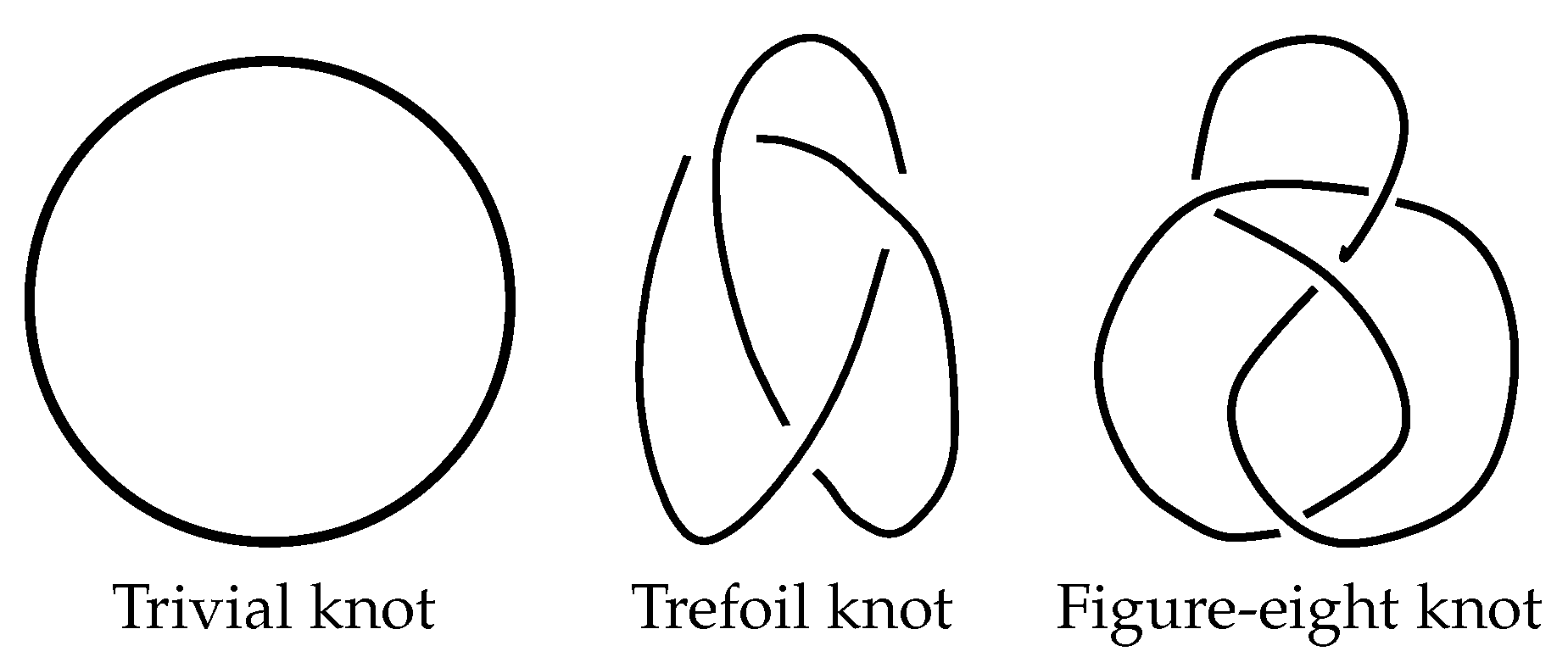
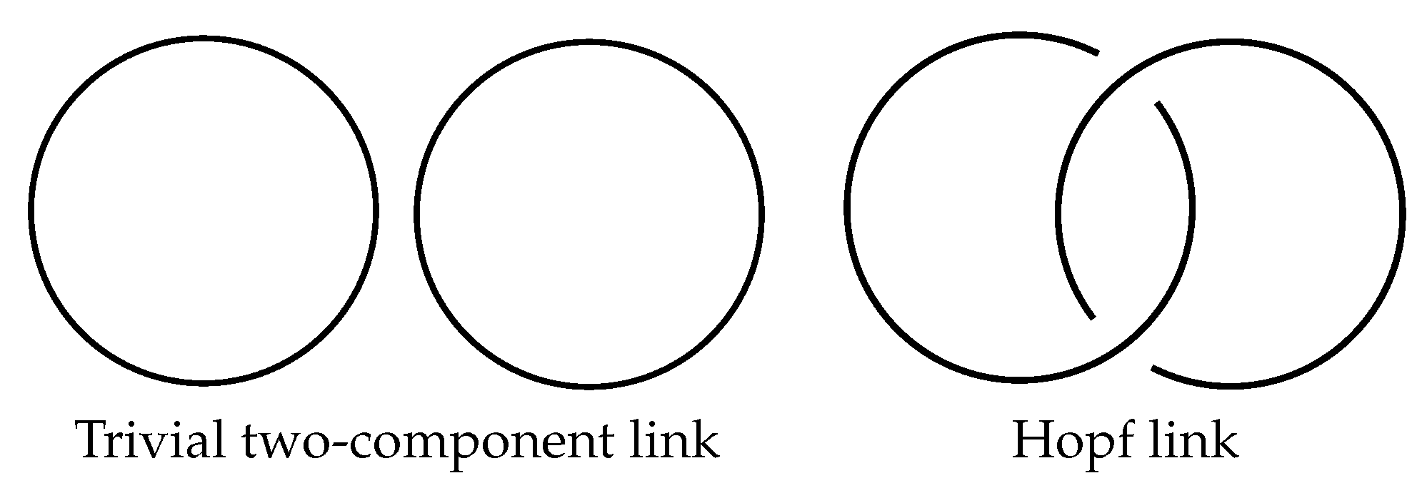
Definition 1.

A knot is a simple, closed curve in the three-space. More precisely, it is the image of an injective, smooth function from the unit circle to ${\mathbb{R}}^3$ with a nonvanishing derivative [18]. You can see some knots in Figure 1:

Definition 2.

An m-component link is a collection of m nonintersecting knots [18]. A trivial two-component link and the Hopf link are given in Figure 2:

Definition 3.

Two links $L_1$ and $L_2$ are said to be isotopic or equivalent if there is a smooth map F: $[0,1]\times S^1\to {\mathbb{R}}^3$, which confirms that $F_t$ is a link for all $t\in [0,1]$ and that that $F_0=L_1$ and $F_1=L_2$. Map F is called isotopy. By the isotopy class of a link L, denoted $\left[L\right]$, we mean the collection of all links that are isotopic to L.

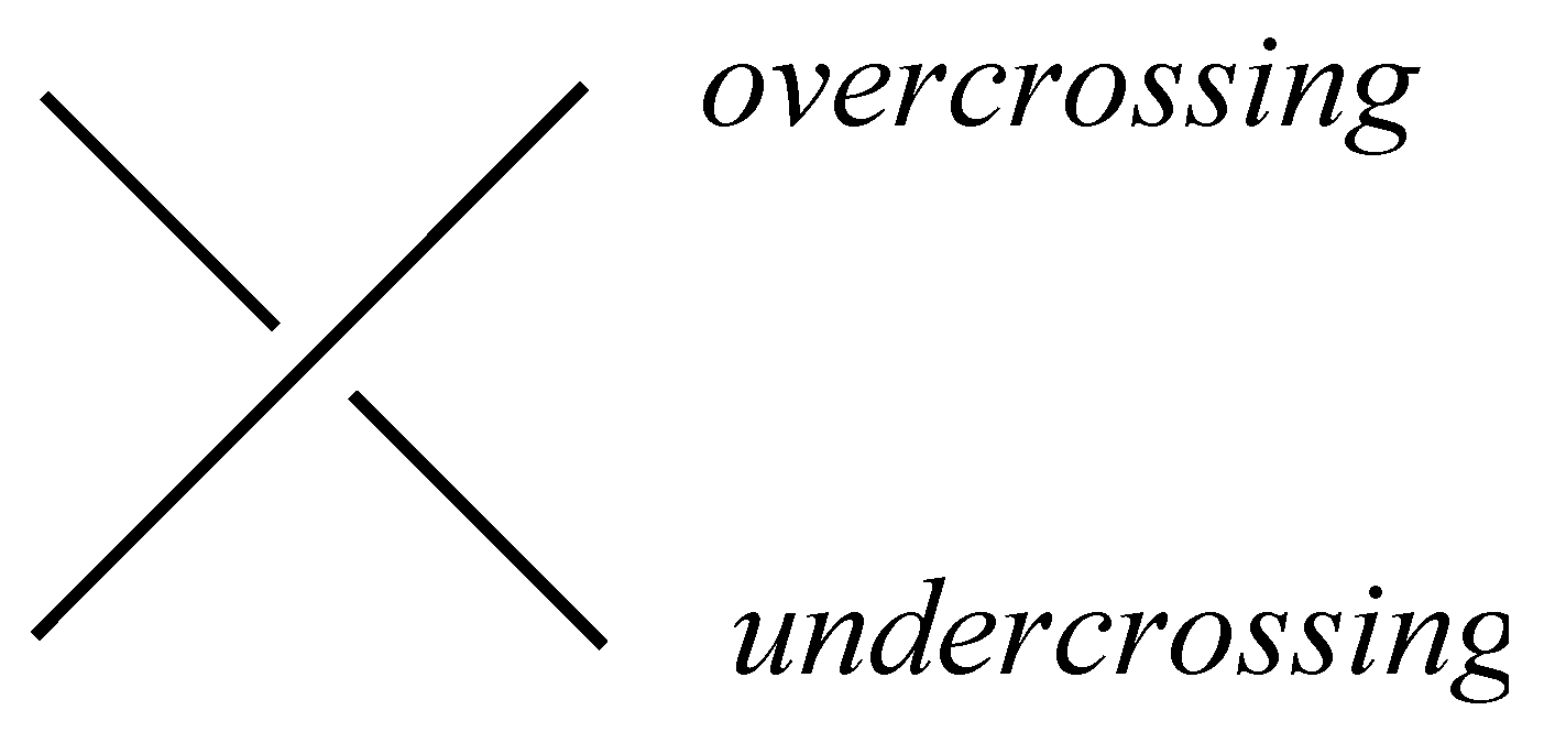
Since it is hard to work with links in ${\mathbb{R}}^3$, people usually prefer working with their projections on a plane. These projections should be generic, which means that all multiple points are double points with a clear information of over- and undercrossing, as you can see in Figure 3. Such a projection of a link is called the diagram of the link.

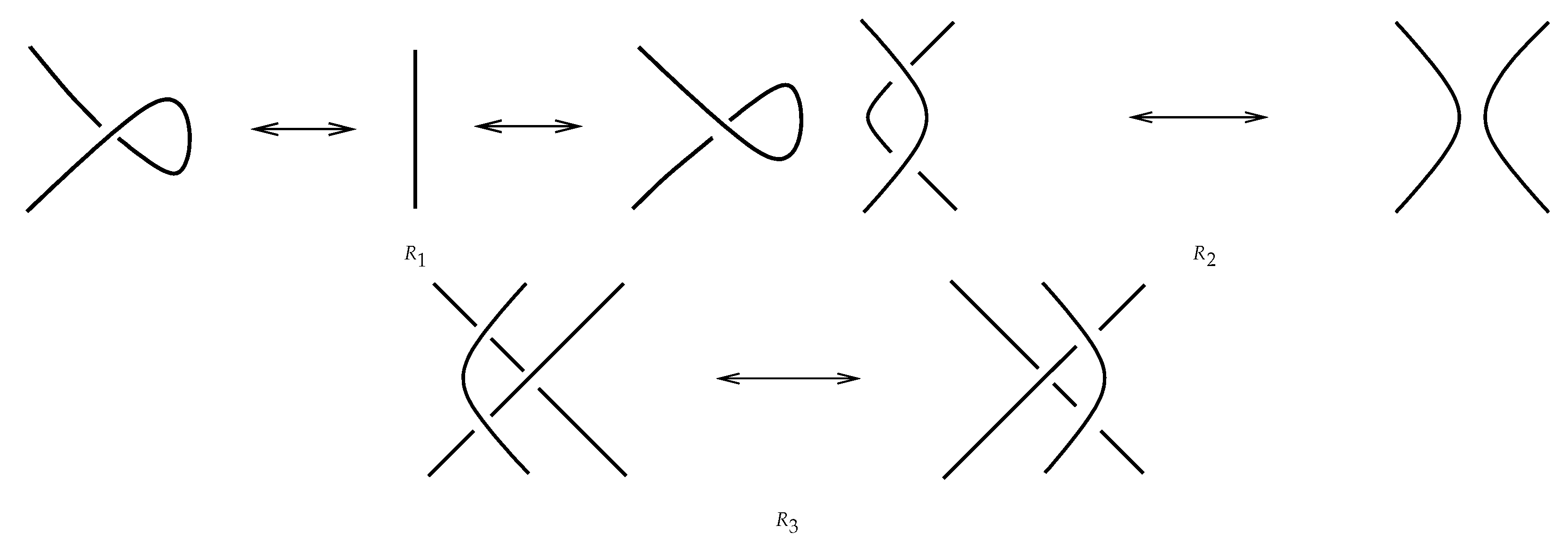
Theorem 1. (Reidemeister, [19]).

Let $D_1$ and $D_2$ be two diagrams of links $L_1$ and $L_2$. Then, links $L_1$ and $L_2$ are isotopic if and only if $D_1$ is transformed into $D_2$ by planar isotopies and by a finite sequence of three local moves represented in Figure 4:

Definition 4.

A link invariant is a function that remains constant on all elements in an isotopy class of a link.

Remark 1.

A function to qualify as a link invariant should be invariant under the Reidemeister moves.

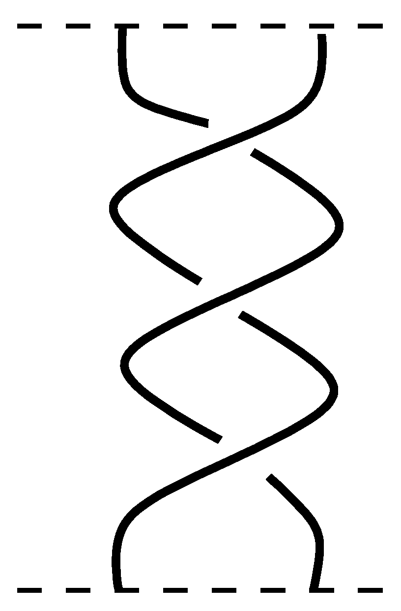
Definition 5.

An n-strand braid is a collection of n nonintersecting, smooth curves joining n points on a plane to n points on another parallel plane in an arbitrary order such that any plane parallel to the given planes intersects exactly n number of curves [20]. The smooth curves are called the strands of the braid. You can see a 2-strand braid in Figure 5:

Definition 6.

The product of two n-strand braids α and β, denoted by $\alpha \beta$, is defined by putting β below α and then gluing their common endpoints.

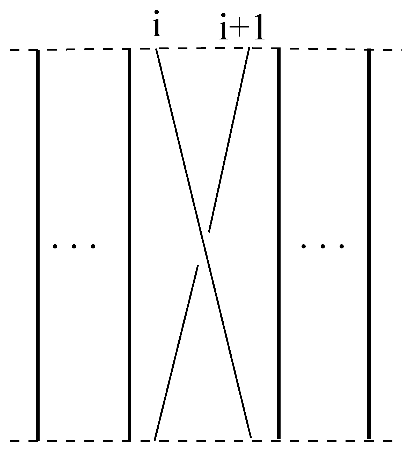
Definition 7.

A braid is said to be elementary if it consists of just one crossing. The ith elementary braid, denoted by $x_i$, is given in Figure 6:

Remark 2.

Each braid is a product of elementary braids.

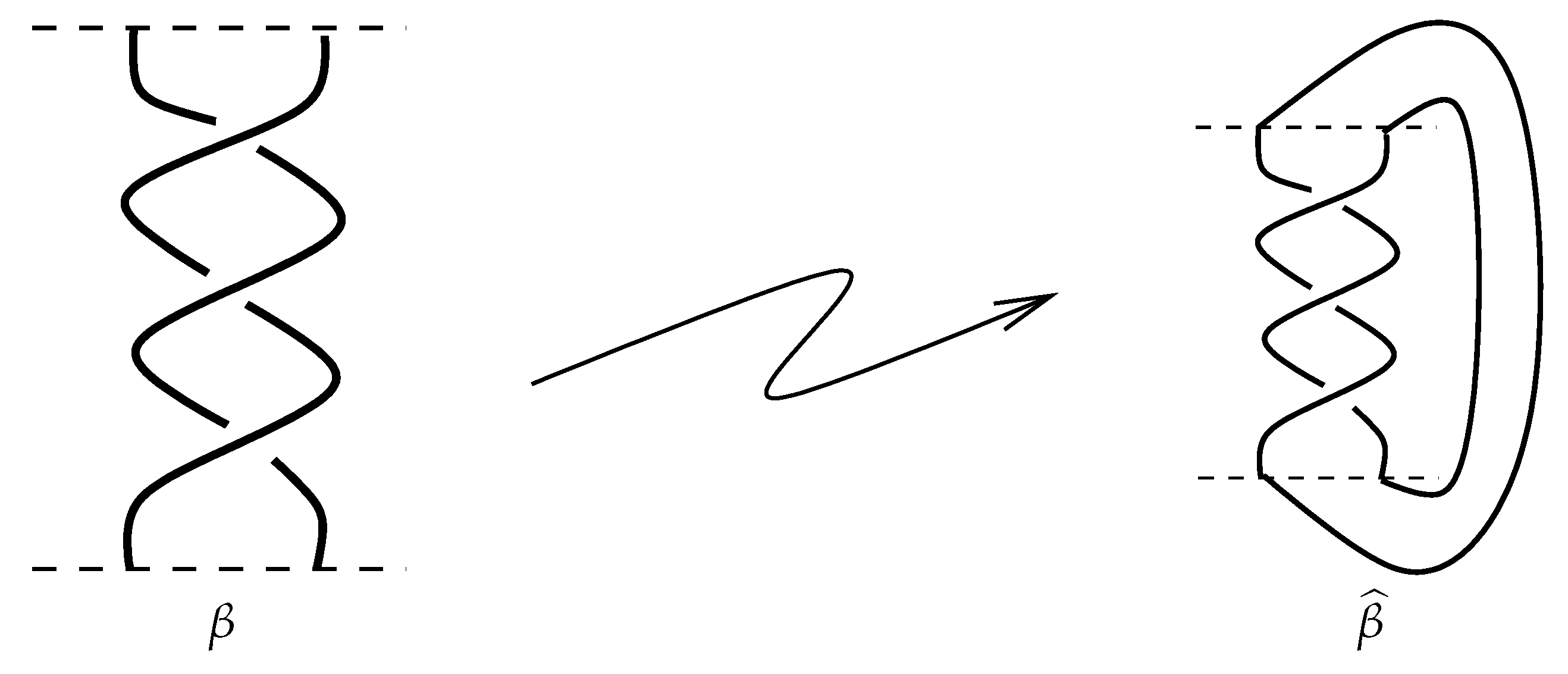
Definition 8.

The closure of a braid β, denoted by $\widehat{\beta }$, is defined by connecting its lower endpoints to its corresponding upper endpoints with smooth curves, as you can see in Figure 7.

Remark 3.

1 

All braids are oriented from top to bottom.

2 

From now onward, by braid β we mean its closure $\widehat{\beta }$, which is actually a link.

An important result by Alexander, connecting links and braids, is:

Theorem 2. (Alexander [21]).

Each link is a closure of some braid.

Definition 9.

The 0- and 1-smoothings of crossing are defined, respectively, by and .

Definition 10.

A collection of disjoint circles obtained by smoothing out all the crossings of a link L is called the Kauffman state of the link [22].

3. Homology

Definition 11.

Let $V={⨁}_n{V}_n,$ be a graded vector space with homogeneous components $\left\{V_n\right\}$ of degree n. The graded dimension of V is the power series $q\dim V$: $={\sum }_n{q}^n\dim V_n$.

Definition 12.

The degree of the tensor product of graded vector space $V_1\otimes V_2$ is the sum of the degrees of the homogeneous components of graded vector spaces $V_1$ and $V_2.$

Remark 4.

In our case, the graded vector space V has the basis $<v_{+},v_{-}>$ with degree $p\left(v_{\pm }\right)=\pm 1$ and the q-dimension $q+q^{-1}.$

Definition 13.

The degree shift $.\left\{l\right\}$ operation on a graded vector space $V=⨁V_n$ is defined by

$${\left(V.\left\{l\right\}\right)}_n=V_{n-l}.$$

Construction of Chain Groups: Let L be a link with n crossings, and let all crossings be labeled from 1 to n. Arrange all its $2^n$ Kauffman states into columns $1,2,\dots ,n$ so that the rth column contains all states having r number of 1-smoothings in it. To every stat $\alpha$ in the rth column we assign graded vector space $V_{\alpha }\left(L\right):=V^{\otimes m}\left\{r\right\}$, where m is the number of circles in $\alpha$. The rth chain group, denoted by ${\left[\left[L\right]\right]}^r:={⨁}_{\alpha :r=\left|\alpha \right|}{V}_{\alpha }\left(L\right)$, is the direct sum of all vector spaces corresponding to all states in the rth column.

Definition 14.

The chain complex $\overline{C}$ of graded vector spaces $\overline{C^r}$ is defined as:

$$\dots \stackrel{}{\to }{\overline{C}}^{r+1}\stackrel{d^{r+1}}{\to }{\overline{C}}^r\stackrel{d^r}{\to }{\overline{C}}^{r-1}\stackrel{d^{r-1}}{\to }\dots$$

such that $d^r\circ d^{r+1}=0$ for each r.

In a system of converting the chain group into a complex, we use the maps between graded vector spaces to satisfy $d\circ d.$ For this purpose we can label the edges of the cube ${\{0,1\}}^{\chi }$ by the sequence $\xi$$ϵ{\{0,1,\star \}}^{\chi }$, where $\xi$ contains only one ⋆ at a time. Here, ⋆ indicates that we change a 1-smoothing to a 0-smoothing. The maps on the edges is denoted by $d_{\xi }$, the height of edges $\left|\xi \right|$. The direct sum of differentials in the cube along the column is

$$d^r:=\sum _{\left|\xi \right|=r}{(-1)}^{\xi }{d}_{\xi }.$$

Now, we discuss the reason behind the sign of ${(-1)}^{\xi }.$ As we want from the differentials to satisfy $d\circ d=0$, the maps $d_{\xi }$ have to anticommute on each of the vertex of the cube. A way to do this is by multiplying edges $d_{\xi }$ by ${(-1)}^{\xi }:={(-1)}^{{\sum }_{i<j}{\xi }_i},$ where j is the location of ⋆ in $\xi .$

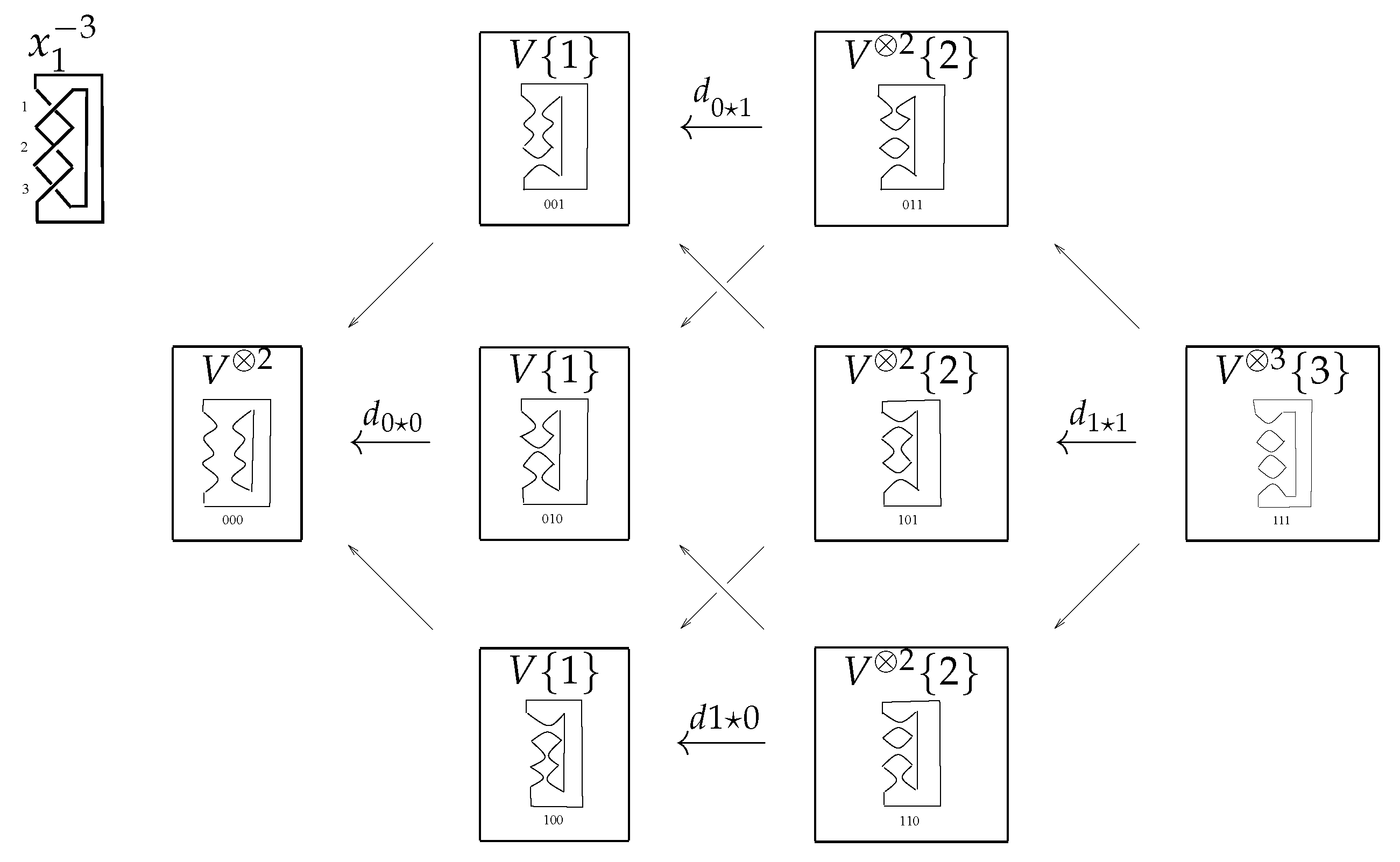
For better understanding, please see the n-cube of trefoil knot $x_1^{-3}$ in Figure 8.

It is useful to note that the ordered basis of V is $〈v_{+},v_{-}〉$ and the ordered basis of $V\otimes V$ is $〈v_{+}\otimes v_{+},v_{-}\otimes v_{+},v_{+}\otimes v_{-},v_{-}\otimes v_{-}〉.$

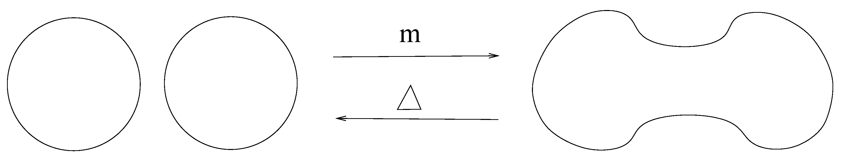
Definition 15.

Linear map $m:V\otimes V\to V$ that merges two circles into a single circle is defined as $m(v_{+}\otimes v_{+})=v_{+},m(v_{+}\otimes v_{-})=v_{-},m(v_{-}\otimes v_{+})=v_{-}$ and $m(v_{-}\otimes v_{-})=0.$

Map $\Delta :V\to V\otimes V$ that divides a circle into two circles is defined as $\Delta \left(v_{+}\right)=v_{+}\otimes v_{-}+v_{-}\otimes v_{+}$ and $\Delta \left(v_{-}\right)=v_{-}\otimes v_{-}$; see Figure 9.

Definition 16.

The homology group associated with the chain complex of a link L is defined as ${\mathcal{H}}^r\left(L\right)=\frac{\ker d^r}{\mathrm{im}{d}^{r+1}}$.

Definition 17.

The kernel of the map $d^r:V^{\otimes r-1}\to V^{\otimes r}$, denoted by $\ker d^r$, is the set of all elements of $V^{\otimes r-1}$ that go to the zero element of $V^{\otimes r}$. The elements of the kernel are called cycles, while the elements of $\mathrm{im}{d}^{r+1}$ are called boundaries.

Remark 5.

Note that the image of the chain complex of $d^{r+1}$ is a subset of kernel $d^r$ as, in general, $d^r\circ d^{r+1}=0.$

Definition 18.

The graded Poincar$\acute{e}$ polynomial $\mathrm{Kh}\left(L\right)$ in variables q and t of the complex is defined as

$$\mathrm{Kh}\left(L\right):=\sum _r{t}^{r}qdim{\mathcal{H}}^r\left(L\right).$$

Theorem 3. (Khovanov [1]).

The graded dimension of homology groups ${\mathcal{H}}^r\left(L\right)$ are link invariants. The graded Poincar$\acute{e}$ polynomial $\mathrm{Kh}\left(L\right)$ is also a link invariant and $\mathrm{Kh}\left(L\right){|}_{t=-1}=\widehat{J}\left(L\right).$

3.1. Homology of $x_1^{-3}$

Now, we give the Khovanov homology of link $x_1^{-3}=$ :

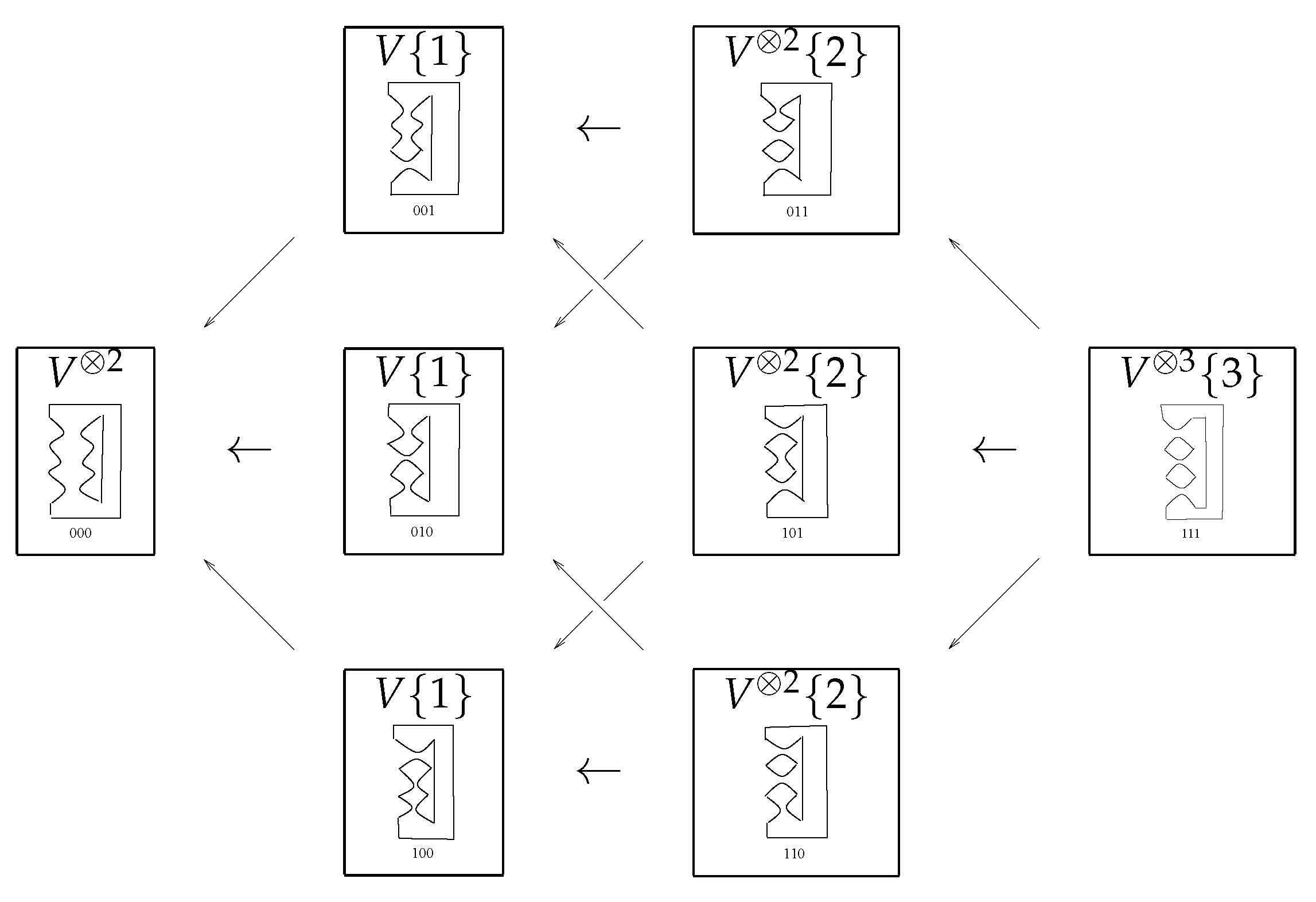
• The n-cube: The 3-cube of $x_1^{-3}$ is given in Figure 10:
• Chain complex: The chain complex of $\widehat{x_1^3}$ is

  $$0\stackrel{d^4}{\to }{V}^{\otimes 3}\stackrel{d^3}{\to }{\oplus }_3{V}^{\otimes 2}\stackrel{d^2}{\to }{\oplus }_{3}V\stackrel{d^1}{\to }{V}^{\otimes 2}\stackrel{d^0}{\to }0.$$
• Ordered basis of the chain complex: The following are the vector spaces of the chain complex along with their ordered bases:

  $$\begin{array}{l}V\otimes V\otimes V=〈v_{+}\otimes v_{+}\otimes v_{+},v_{-}\otimes v_{+}\otimes v_{+},v_{+}\otimes v_{-}\otimes v_{+},v_{+}\otimes v_{+}\otimes v_{-},v_{-}\otimes v_{-}\otimes v_{+},v_{-}\otimes v_{+}\otimes v_{-},v_{+}\otimes v_{-}\otimes v_{-},v_{-}\otimes v_{-}\otimes v_{-}〉\\ (V\otimes V)\oplus (V\otimes V)\oplus (V\otimes V)=〈(v_{+}\otimes v_{+},0,0),(0,v_{+}\otimes v_{+},0),(0,0,v_{+}\otimes v_{+}),(v_{-}\otimes v_{+},0,0),(0,v_{-}\otimes v_{+},0),(0,0,v_{-}\otimes v_{+}),(v_{+}\otimes v_{-},0,0),(0,v_{+}\otimes v_{-},0),(0,0,v_{+}\otimes v_{-}),(v_{-}\otimes v_{-},0,0)(0,v_{-}\otimes v_{-},0),(0,0,v_{-}\otimes v_{-})〉\\ V\oplus V\oplus V=〈(v_{+},0,0),(0,v_{+},0),(0,0,v_{+}),(v_{-},0,0),(0,v_{-},0),(0,0,v_{-})〉\\ V\otimes V=〈v_{+}\otimes v_{+},v_{-}\otimes v_{+},v_{+}\otimes v_{-},v_{-}\otimes v_{-}〉\end{array}$$
• Differential maps in matrix form: Differential map $d^3\left(V_1\otimes V_2\otimes V_3\right)=\left(m(v_1\otimes v_2)\otimes v_3,v_1\otimes m(v_2\otimes v_3),v_2\otimes m(v_1\otimes v_3)\right)$ in terms of a matrix is:

  $$d^3=\left(\begin{array}{cccccccc}1& 0& 0& 0& 0& 0& 0& 0\\ 1& 0& 0& 0& 0& 0& 0& 0\\ 1& 0& 0& 0& 0& 0& 0& 0\\ 0& 1& 1& 0& 0& 0& 0& 0\\ 0& 1& 0& 0& 0& 0& 0& 0\\ 0& 0& 1& 0& 0& 0& 0& 0\\ 0& 0& 0& 1& 0& 0& 0& 0\\ 0& 0& 1& 1& 0& 0& 0& 0\\ 0& 1& 0& 1& 0& 0& 0& 0\\ 0& 0& 0& 0& 0& 1& 1& 0\\ 0& 0& 0& 0& 1& 1& 0& 0\\ 0& 0& 0& 0& 1& 0& 1& 0\end{array}\right),$$

  and map $d^2\left(V_1\otimes V_2,V_3\otimes V_4,V_5\otimes V_6\right)=\left(m(v_3\otimes v_4)-m(v_1\otimes v_2),m(v_5\otimes v_6)-m(v_1\otimes v_2),m(v_5\otimes v_6)-m(v_3\otimes v_4)\right)$ is $d^2=\left(\begin{array}{cccc}A& 0& 0& 0\\ 0& A& A& 0\end{array}\right),$ where $A=\left(\begin{array}{ccc}-1& 1& 0\\ -1& 0& 1\\ 0& -1& 1\end{array}\right).$ Also, $d^1\left(V_1,V_2,V_3\right)=\Delta \left(v_1\right)-\Delta \left(v_2\right)+\Delta \left(v_3\right)$ is $d^1=\left(\begin{array}{cccccc}0& 0& 0& 0& 0& 0\\ 1& -1& 1& 0& 0& 0\\ 1& -1& 1& 0& 0& 0\\ 0& 0& 0& 1& -1& 1\end{array}\right).$
• Khovanov Homology: On solving $d^{3}x=0$ or

  $$\left(\begin{array}{cccccccc}1& 0& 0& 0& 0& 0& 0& 0\\ 1& 0& 0& 0& 0& 0& 0& 0\\ 1& 0& 0& 0& 0& 0& 0& 0\\ 0& 1& 1& 0& 0& 0& 0& 0\\ 0& 1& 0& 0& 0& 0& 0& 0\\ 0& 0& 1& 0& 0& 0& 0& 0\\ 0& 0& 0& 1& 0& 0& 0& 0\\ 0& 0& 1& 1& 0& 0& 0& 0\\ 0& 1& 0& 1& 0& 0& 0& 0\\ 0& 0& 0& 0& 0& 1& 1& 0\\ 0& 0& 0& 0& 1& 1& 0& 0\\ 0& 0& 0& 0& 1& 0& 1& 0\end{array}\right)\left(\begin{array}{c}{x}_1\\ x_2\\ x_3\\ x_4\\ x_5\\ x_6\\ x_7\\ x_8\end{array}\right)=0,$$

  we receive $x_1=x_2=x_3=x_4=0,$ $x_2+x_3=0,$ $x_3+x_4=0,$ $x_2+x_4=0,$ $x_6+x_7=0,$ $x_5+x_6=0,$ and $x_5+x_7=0.$ So the kernel of $d^3=〈\left[\begin{array}{c}0\\ 0\\ 0\\ 0\\ 0\\ 0\\ 0\\ 1\end{array}\right]〉$. Similarly, the image of $d^3$ is

  $$〈\left[\begin{array}{c}1\\ 1\\ 1\\ 0\\ 0\\ 0\\ 0\\ 0\\ 0\\ 0\\ 0\\ 0\end{array}\right],\left[\begin{array}{c}0\\ 0\\ 0\\ 1\\ 1\\ 0\\ 0\\ 0\\ 1\\ 0\\ 0\\ 0\end{array}\right],\left[\begin{array}{c}0\\ 0\\ 0\\ 1\\ 0\\ 1\\ 0\\ 1\\ 0\\ 0\\ 0\\ 0\end{array}\right],\left[\begin{array}{c}0\\ 0\\ 0\\ 0\\ 0\\ 0\\ 1\\ 1\\ 1\\ 0\\ 0\\ 0\end{array}\right],\left[\begin{array}{c}0\\ 0\\ 0\\ 0\\ 0\\ 0\\ 0\\ 0\\ 0\\ 0\\ 1\\ 1\end{array}\right],\left[\begin{array}{c}0\\ 0\\ 0\\ 0\\ 0\\ 0\\ 0\\ 0\\ 0\\ 1\\ 1\\ 0\end{array}\right],\left[\begin{array}{c}0\\ 0\\ 0\\ 0\\ 0\\ 0\\ 0\\ 0\\ 0\\ 1\\ 0\\ 1\end{array}\right]〉.$$

  Thus,

  $$\begin{array}{ccc}\hfill {\mathcal{H}}^3\left(\widehat{x_1^3}\right)& =& \frac{\ker d^3}{\mathrm{im}{d}^4}=\frac{{\mathbb{Z}}_{(v_{-}\otimes v_{-}\otimes v_{-})}}{0}={\mathbb{Z}}_{(v_{-}\otimes v_{-}\otimes v_{-})}.\hfill \end{array}$$

  To compute the homology of the next level, we first cancel out the terms that appear in both $\ker d^2$ and $\mathrm{im}{d}^3$, and then use a special trick: Note that the last three summands of $\ker d^2$ make up all of ${\mathbb{Z}}_{(v_{-}\otimes v_{-})}^3$, where the last three summands of $\mathrm{im}{d}^3$ span the subspace of ${\mathbb{Z}}_{(v_{-}\otimes v_{-})}^3$ generated by vectors $(0,1,1)$, $(1,1,0)$ and $(1,0,1)$. Now, form a matrix whose columns are these vectors. Since the eigenvalues of this matrix are $-1,1$, and 2, we can write:

  $$\frac{{\mathbb{Z}}^3}{\langle (0,1,1),(1,1,0),(1,0,1)\rangle }=\frac{\mathbb{Z}}{2\mathbb{Z}}\oplus \frac{\mathbb{Z}}{{\mathbb{Z}}_1}\oplus \frac{\mathbb{Z}}{{\mathbb{Z}}_{-1}}={\mathbb{Z}}_2.$$

  Reducing the remaining matrices of kernel of $d^2$ and image of $d^3$ into reduced row echelon form, quotient $\frac{\ker d^2}{\mathrm{im}{d}^3}$ becomes isomorphic to $\mathbb{Z}$. Hence,

  $$\begin{array}{ccc}\hfill {\mathcal{H}}^2\left(\widehat{x_1^3}\right)& =& \frac{\ker d^2}{\mathrm{im}{d}^3}=\mathbb{Z}\oplus {\mathbb{Z}}_2.\hfill \end{array}$$

  The range of $d^2$ is ${\mathbb{Z}}_{(v_{+},v_{+},0)}\oplus {\mathbb{Z}}_{(v_{+},0,-v_{+})}\oplus {\mathbb{Z}}_{(0,v_{+},v_{+})}\oplus {\mathbb{Z}}_{(v_{-},v_{-},0)}\oplus {\mathbb{Z}}_{(v_{-},0,-v_{-})}\oplus {\mathbb{Z}}_{(0,v_{-},v_{-})}$ and the kernel of $d^1$ is ${\mathbb{Z}}_{(v_{+},v_{+},0)}\oplus {\mathbb{Z}}_{(0,v_{+},v_{+})}\oplus {\mathbb{Z}}_{(v_{+},0,-v_{+})}\oplus {\mathbb{Z}}_{(v_{-},v_{-},0)}\oplus {\mathbb{Z}}_{(0,v_{-},v_{-})}\oplus {\mathbb{Z}}_{(v_{-},0,-v_{-})}.$ Since $\ker d^1=\mathrm{im}{d}^2$,

  $${\mathcal{H}}^1\left(\widehat{x_1^3}\right)=0.$$

  It is clear from the chain complex that the kernel of $d^0$ is the full space $V\otimes V.$

  $${\mathcal{H}}^0\left(\widehat{x_1^3}\right)=\frac{{\mathbb{Z}}_{(v_{+}\otimes v_{+})}\oplus {\mathbb{Z}}_{(v_{-}\otimes v_{+})}\oplus {\mathbb{Z}}_{(v_{+}\otimes v_{-})}\oplus {\mathbb{Z}}_{(v_{-}\otimes v_{-})}}{{\mathbb{Z}}_{(v_{-}\otimes v_{+}+v_{+}\otimes v_{-})}\oplus {\mathbb{Z}}_{(v_{-}\otimes v_{-})}}={\mathbb{Z}}_{(v_{+}\otimes v_{+})}\oplus \mathbb{Z}.$$

3.2. Homology of ${\Delta }^{2k+1}$

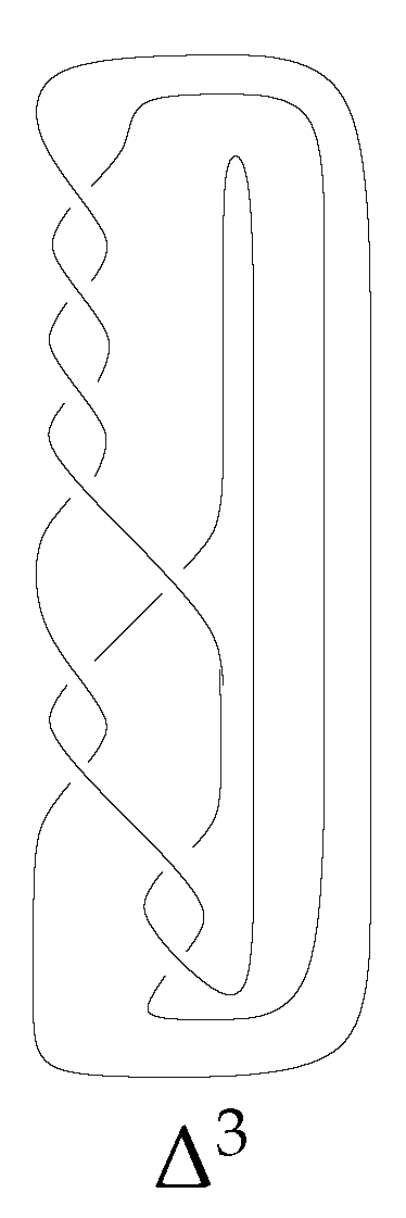
We now compute the homology of braid link ${\Delta }^{2k+1}$, where $\Delta =x_1{x}_2{x}_1$. The canonical form of this braid is ${\Delta }^{2k+1}=x_1^{2k+2}{x}_2{x}_1^2{x}_2^2{x}_1^2\cdots x_2^2{x}_1^2{x}_1^2$, having $2k+2$ factors; you can see ${\Delta }^3$ in Figure 11.

The co-chain complex of the link ${\Delta }^{2k+1}$ is $0\stackrel{d^{-1}}{\to }{V}^{\otimes 3}\stackrel{d^0}{\to }{\oplus }_{6k+3}{V}^{\otimes 2}\stackrel{d^1}{\to }{\oplus }_{\left(\genfrac{}{}{0pt}{}{2k+1}{1}\right)\left(\genfrac{}{}{0pt}{}{4k+2}{1}\right)}{V}^{\otimes 1}{\oplus }_{\left(\genfrac{}{}{0pt}{}{2k+1}{1}\right)+\left(\genfrac{}{}{0pt}{}{4k+2}{2}\right)}{V}^{\otimes 3}$$\stackrel{d^3}{\to }{\oplus }_{\left(\genfrac{}{}{0pt}{}{2k+1}{1}\right)\left(\genfrac{}{}{0pt}{}{4k+2}{2}\right)+\left(\genfrac{}{}{0pt}{}{2k+1}{2}\right)\left(\genfrac{}{}{0pt}{}{4k+2}{1}\right)}{V}^{\otimes 1}{\oplus }_{\left(\genfrac{}{}{0pt}{}{2k+1}{1}\right)+\left(\genfrac{}{}{0pt}{}{4k+2}{2}\right)}{V}^{\otimes 3}\stackrel{d^4}{\to }\dots$$\stackrel{d^{6k+1}}{\to }{\oplus }_{\left(\genfrac{}{}{0pt}{}{4k+2}{1}\right)}{V}^{\otimes 2k+1}{\oplus }_{\left(\genfrac{}{}{0pt}{}{2k+1}{1}\right)}{V}^{\otimes 2k+3}\stackrel{d^{6k+2}}{\to }{V}^{\otimes 2k+2}\stackrel{d^{6k+3}}{\to }0.$

We now represent the differential maps in terms of matrices. The matrix representing differential $d^0$ has order $24k+12\times 8$ and is

$$d^0=\left(\begin{array}{cccccccc}A& 0& 0& 0& 0& 0& 0& 0\\ 0& A& B& 0& 0& 0& 0& 0\\ 0& 0& C& A& 0& 0& 0& 0\\ 0& 0& 0& 0& C& A& B& 0\end{array}\right).$$

Here, each matrix $A,B$, and C has a $(6k+3)\times 1$ order:

$$\begin{array}{ccc}\hfill A& =& {\left(\begin{array}{ccccccccc}1& 1& 1& 1& 1& 1& 1& \cdots & 1\end{array}\right)}^t\hfill \\ \hfill B& =& {\left(\begin{array}{cccccccccc}0& 1& 0& 0& 1& 0& 0& \cdots & 1& 0\end{array}\right)}^t\hfill \\ \hfill C& =& {\left(\begin{array}{cccccccccc}1& 0& 1& 1& 0& 1& 1& \cdots & 0& 1\end{array}\right)}^t\hfill \end{array}$$

Since $\ker d^0={\mathbb{Z}}_{v_{-}\otimes v_{-}\otimes v_{-}}\oplus {\mathbb{Z}}_{v_{+}\otimes v_{-}\otimes v_{-}-v_{-}\otimes v_{+}\otimes v_{-}+v_{+}\otimes v_{-}\otimes v_{-}}$ and $\mathrm{im}{d}^{-1}=0$, the homology at this level is

$${\mathcal{H}}^0\left({\Delta }^{2k+1}\right)={\mathbb{Z}}_{v_{-}\otimes v_{-}\otimes v_{-}}\oplus {\mathbb{Z}}_{v_{+}\otimes v_{-}\otimes v_{-}-v_{-}\otimes v_{+}\otimes v_{-}+v_{+}\otimes v_{-}\otimes v_{-}}.$$

Now, we go for differential map $d^1$. The matrix that represents it has an order of $20(6k^2+3)\times 4(6k+3)$ and is

$$d^1=\left(\begin{array}{cccc}{R}_1& 0& 0& 0\\ 0& R_1& R_1& 0\\ 0& 0& 0& 0\\ 0& 0& 0& 0\\ 0& 0& 0& 0\\ R_2& 0& 0& 0\\ R_2& 0& 0& 0\\ 0& R_2& 0& 0\\ 0& 0& R_2& 0\\ 0& 0& 0& R_2\\ 0& R_3& R_4& 0\\ ⋮& ⋮& \ddots & ⋮\\ 0& 0& R_{n-1}& R_n\end{array}\right).$$

The order of each of the matrix $R_i$ is $(12k+6)\times (6k+3)$:

$$R_1=\left(\begin{array}{cccccccc}1& -1& 0& 0& 0& \dots & 0& 0\\ 1& 0& 0& 0& -1& 0& \dots & 0\\ 1& 0& 0& 0& 0& 0& \dots & -1\\ 0& 1& -1& 0& 0& 0& \dots & 0\\ 0& 1& 0& -1& 0& 0& \dots & 0\\ 0& 1& 0& 0& 0& -1& \dots & 0\\ 0& 1& 0& 0& 0& 0& \dots & -1\\ ⋮& ⋮& ⋮& ⋮& ⋮& ⋮& ⋮& ⋮\\ 0& 0& 0& 0& 0& \dots & 1& -1\end{array}\right),$$

$$R_2=\left(\begin{array}{cccccccc}1& 0& -1& 0& 0& \dots & 0& 0\\ 1& 0& \dots & -1& 0& 0& 0& 0\\ 1& 0& \dots & 0& 0& -1& 0& 0\\ 1& 0& \dots & 0& 0& 0& -1& 0\\ 1& 0& \dots & 0& 0& 0& 0& -1\\ 0& 1& 0& 0& -1& 0& \dots & 0\\ 0& 1& \dots & 0& 0& -1& 0& 0\\ ⋮& ⋮& ⋮& ⋮& ⋮& ⋮& ⋮& ⋮\\ 0& 0& 0& 0& \dots & 1& 0& -1\end{array}\right),$$

$$R_3=\left(\begin{array}{cccccccc}1& 0& -1& 0& 0& \dots & 0& 0\\ 1& 0& \dots & -1& 0& 0& 0& 0\\ 1& 0& \dots & 0& 0& -1& 0& 0\\ 1& 0& \dots & 0& 0& 0& -1& 0\\ 1& 0& \dots & 0& 0& 0& 0& -1\\ 0& 0& 1& -1& 0& 0& \dots & 0\\ 0& 0& 1& 0& 0& -1& \dots & 0\\ 0& 0& 1& 0& \dots & -1& 0& 0\\ 0& 0& 1& 0& \dots & 0& 0& -1\\ ⋮& ⋮& ⋮& ⋮& ⋮& ⋮& ⋮& ⋮\\ 0& 0& 0& 0& \dots & 1& 0& -1\end{array}\right),$$

$$R_4=\left(\begin{array}{cccccccc}0& 0& 0& 0& 0& \dots & 0& 0\\ ⋮& ⋮& ⋮& ⋮& ⋮& ⋮& ⋮& ⋮\\ 0& 1& 0& 0& -1& 0& \dots & 0\\ 0& 1& \dots & 0& 0& -1& 0& 0\\ ⋮& ⋮& ⋮& ⋮& ⋮& ⋮& ⋮& ⋮\\ 0& 0& 0& 0& 1& 0& \dots & -1\end{array}\right),$$

and, at the end, all rows of matrix $R_n$ are zero except for the last row, which is

$$\left(\begin{array}{cccccccc}0& \dots & 0& 0& 1& 0& \dots & -1\end{array}\right).$$

Here, $\ker d^1={\mathbb{Z}}_{(v_{+}\otimes v_{+}+v_{+}\otimes v_{+}+v_{+}\otimes v_{+}+v_{+}\otimes v_{+}+v_{+}\otimes v_{+}+v_{+}\otimes v_{+}+v_{+}\otimes v_{+}+v_{+}\otimes v_{+})}\oplus {\mathbb{Z}}_{(v_{+}\otimes v_{-}+v_{+}\otimes v_{-}+v_{+}\otimes v_{-}+v_{+}\otimes v_{-}+v_{+}\otimes v_{-}+v_{+}\otimes v_{-}+v_{+}\otimes v_{-}+v_{+}\otimes v_{-})}\oplus {\mathbb{Z}}_{(v_{-}\otimes v_{+}+v_{-}\otimes v_{+}-v_{+}\otimes v_{-}-v_{+}\otimes v_{-}-v_{+}\otimes v_{-})}\oplus {\mathbb{Z}}_{(v_{+}\otimes v_{-}+v_{+}\otimes v_{-}+v_{+}\otimes v_{-}+v_{-}\otimes v_{+}+v_{-}\otimes v_{+}+v_{-}\otimes v_{+}+v_{-}\otimes v_{+}+v_{-}\otimes v_{+})}\oplus {\mathbb{Z}}_{(v_{-}\otimes v_{-}+v_{-}\otimes v_{-})}\oplus {\mathbb{Z}}_{(v_{-}\otimes v_{-}+v_{-}\otimes v_{-}+v_{-}\otimes v_{-}+v_{-}\otimes v_{-}+v_{-}\otimes v_{-})}$ and $\mathrm{im}{d}^0={\mathbb{Z}}_{(v_{+}\otimes v_{+})}\oplus {\mathbb{Z}}_{(v_{+}\otimes v_{-})}\oplus {\mathbb{Z}}_{(v_{-}\otimes v_{+})}\oplus {\mathbb{Z}}_{(v_{-}\otimes v_{-})}\oplus {\mathbb{Z}}_{(v_{+}\otimes v_{+})}\oplus {\mathbb{Z}}_{(v_{+}\otimes v_{-})}\oplus {\mathbb{Z}}_{(v_{-}\otimes v_{+})}$.

Since the number of $\mathbb{Z}$ spaces appear in the kernel of $d^1$, it is exactly the same as the image of $d^0$, ${\mathcal{H}}^1\left({\Delta }^{2k+1}\right)=0.$

The image of $d^1$ is obvious. We just need the kernel of $d^2$. The matrix that represents $d^2$ has an order of $(2^{6k+3}+2^{2k+2})(6k+5)\times 20(6k^2+3)$ and is

$$\left(\begin{array}{ccccccccccc}{S}_1& S_2& S_3& S_4& S_5& S_6& S_7& S_8& S_9& \dots & S_{20}\\ S_{21}& S_{21}& S_{22}& S_{23}& S_{24}& S_{25}& S_{26}& S_{27}& S_{28}& \dots & S_{40}\\ ⋮& ⋮& ⋮& ⋮& ⋮& ⋮& ⋮& ⋮& ⋮& ⋮& ⋮\\ S_{n-19}& S_{n-18}& S_{n-17}& S_{n-16}& S_{n-15}& S_{n-14}& S_{n-13}& S_{n-12}& S_{n-11}& \dots & S_n\end{array}\right).$$

Here, the order of each $S_i$ is $(4k^2+3)\times (6k^2+3)$, and is:

$$S_1=\left(\begin{array}{cccccccc}0& -1& 0& 0& 0& 0& \dots & 0\\ 1& 0& 0& 0& 0& 0& \dots & 1\\ 1& 0& 0& 0& 0& 0& \dots & 1\\ 0& 0& 0& 0& 0& 0& \dots & 0\\ 0& 0& -1& 0& 0& 0& \dots & 0\\ 1& 0& 0& 0& 0& 0& \dots & 0\\ 1& 0& 0& 0& 0& 0& \dots & 0\\ ⋮& ⋮& ⋮& ⋮& ⋮& ⋮& ⋮& ⋮\\ 0& 0& 0& 0& 0& 0& \dots & 0\end{array}\right),S_2=\left(\begin{array}{cccccccc}0& 0& 0& 0& 0& 0& \dots & 0\\ 0& 0& 0& 0& 0& 0& \dots & 0\\ 0& 0& 0& 0& 0& 0& \dots & 0\\ 0& 0& 0& 0& 0& 0& \dots & 0\\ 0& 0& 0& 0& 0& 0& \dots & 0\\ 1& 0& 0& 0& 0& 0& \dots & 0\\ ⋮& ⋮& ⋮& ⋮& ⋮& ⋮& ⋮& ⋮\\ 1& 0& 0& 0& 0& 0& \dots & 0\end{array}\right),$$

$$S_3=\left(\begin{array}{cccccccc}0& 0& 0& 0& 0& 0& \dots & 0\\ 0& -1& 0& 0& 0& 0& \dots & 0\\ 0& 0& 0& 0& 0& 0& \dots & 0\\ 1& 0& 0& 0& 0& 0& \dots & 1\\ 0& 0& -1& 0& 0& 0& \dots & 0\\ 0& 0& 0& 0& 0& 0& \dots & 0\\ ⋮& ⋮& ⋮& ⋮& ⋮& ⋮& ⋮& ⋮\\ 0& 0& 0& 0& 0& 0& \dots & 0\end{array}\right),S_4=\left(\begin{array}{cccccccc}0& 0& 0& 0& 0& 0& \dots & 0\\ 0& 0& 0& 0& 0& 0& \dots & 0\\ -1& 0& 0& 0& 0& 0& \dots & 0\\ 0& 0& 0& 0& 0& 0& \dots & 0\\ 0& 0& 0& 0& 0& 0& \dots & 0\\ 0& 0& 0& 0& 0& 0& \dots & 0\\ 0& -1& 0& 0& 0& 0& \dots & 0\\ ⋮& ⋮& ⋮& ⋮& ⋮& ⋮& ⋮& ⋮\\ 0& 0& 0& 0& 0& 0& \dots & 0\end{array}\right),$$

$$⋮$$

$$S_{n-2}=\left(\begin{array}{cccccccc}0& 0& 0& 0& 0& 0& \dots & 0\\ 0& 0& 0& 0& 0& 0& \dots & 0\\ 0& 0& -1& 0& 0& 0& \dots & 0\\ 0& 0& 0& 0& 0& 0& \dots & 0\\ 0& 0& 0& 0& 0& 0& \dots & 0\\ 0& 0& 0& 0& 0& 0& \dots & 0\\ ⋮& ⋮& ⋮& ⋮& ⋮& ⋮& ⋮& ⋮\\ 0& 0& 0& 0& 0& 0& \dots & 0\end{array}\right),$$

$$S_{n-1}=\left(\begin{array}{cccccccc}0& 0& 0& 0& 0& 0& \dots & 0\\ 0& 0& 0& 0& 0& 0& \dots & 0\\ 0& 0& 0& 0& 0& 0& \dots & 0\\ -1& 0& 0& 0& 0& 0& \dots & -1\\ 0& 0& 0& 0& 0& 0& \dots & 0\\ 0& 0& 0& 0& 0& 0& \dots & 0\\ ⋮& ⋮& ⋮& ⋮& ⋮& ⋮& ⋮& ⋮\\ 0& -1& 0& 0& 0& 0& \dots & 0\end{array}\right),$$

$$S_n=\left(\begin{array}{cccccccc}0& 0& 0& 0& 0& 0& \dots & 0\\ 0& 0& 0& 0& 0& 0& \dots & 0\\ 0& 0& 0& 0& 0& 0& \dots & 0\\ 0& 0& 0& 0& 0& 0& \dots & 0\\ 0& 0& 0& 0& 0& 0& \dots & 0\\ 0& 0& 0& 0& 0& 0& \dots & 0\\ ⋮& ⋮& ⋮& ⋮& ⋮& ⋮& ⋮& ⋮\\ -1& 0& 0& 0& 0& 0& \dots & 0\end{array}\right).$$

Thus, ${\mathcal{H}}^2\left({\Delta }^{2k+1}\right)=\mathbb{Z}\oplus \mathbb{Z}$. Differential $d^{6k+2}$ of order $\left(2^{2k+2}\right)\times (2k+1)(2^{2k+2}+2^{2k+3})$ is

$$d^{6k+2}=\left(\begin{array}{ccccccc}{Y}_1& Y_2& Y_3& Y_4& Y_5& \dots & Y_{6k+3}\end{array}\right),$$

where $Y_i$ are matrices, each having an order of $2^{2k+2}\times 2^{2k+2}:$

$$Y_1=\left(\begin{array}{cccccccc}0& -1& 0& 0& 1& 0& \cdots & 0\\ 0& 0& 0& 0& 0& 0& \cdots & 0\\ ⋮& ⋮& ⋮& ⋮& ⋮& ⋮& ⋮& ⋮\\ 0& 0& 1& -1& 0& -1& \cdots & 0\\ 1& 0& 1& -1& 0& -1& \cdots & 0\\ 1& 0& 0& 0& 0& 0& \cdots & -1\\ 0& 0& 0& 0& 0& 0& \cdots & -1\\ ⋮& ⋮& ⋮& ⋮& ⋮& ⋮& ⋮& ⋮\\ 0& 0& 0& 0& 0& 0& \cdots & 0\end{array}\right),$$

$$Y_2=\left(\begin{array}{ccccccccc}0& 0& \cdots & 0& 0& 0& 0& 0& 0\\ -1& 0& \cdots & 0& 0& 0& 0& 0& 0\\ ⋮& ⋮& ⋮& ⋮& ⋮& ⋮& ⋮& ⋮& ⋮\\ 0& 1& \cdots & 1& 0& -1& 0& 0& 1\\ 0& 1& \cdots & 1& 0& 0& 1& -1& 0\\ 0& 0& \cdots & 0& 1& 0& 1& -1& 0\end{array}\right),$$

$$Y_3=\left(\begin{array}{ccccccccc}0& 0& 0& 0& 0& 0& 0& 0& \cdots \\ 0& 0& 0& 0& 0& 0& 0& 0& \cdots \\ 0& 0& -1& 0& 0& 0& 0& 0& \cdots \\ 0& 0& 0& 0& 0& -1& 0& 0& \cdots \\ ⋮& ⋮& ⋮& ⋮& ⋮& ⋮& ⋮& ⋮& ⋮\\ -1& 1& 0& 0& 0& 0& 0& 0& \cdots \\ -1& 1& 0& 1& 0& 0& 1& -1& \cdots \end{array}\right),$$

$$Y_4=\left(\begin{array}{cccccccc}0& 0& 0& 0& 0& 0& 0& \cdots \\ 0& 0& 0& 0& 0& 0& 0& \cdots \\ ⋮& ⋮& ⋮& ⋮& ⋮& ⋮& ⋮& ⋮\\ 0& 1& 0& 0& -1& 0& 0& \cdots \\ 0& 0& 0& 0& 0& 0& 0& \cdots \\ -1& 0& -1& 1& 0& 0& 0& \cdots \\ -1& 0& -1& 1& 0& 0& 0& \cdots \\ ⋮& ⋮& ⋮& ⋮& ⋮& ⋮& ⋮& ⋮\\ 0& 0& 0& 0& 0& 0& 1& \cdots \end{array}\right),$$

$$⋮$$

$$Y_i=\left(\begin{array}{ccccccccc}0& 0& 0& 0& 0& 0& 0& 0& \cdots \\ 0& 0& 0& 0& 0& 0& 0& 0& \cdots \\ ⋮& ⋮& ⋮& ⋮& ⋮& ⋮& ⋮& ⋮& ⋮\\ 0& -1& 0& 0& 0& 0& 0& 0& \cdots \\ 0& 0& 0& 0& 0& 0& 0& 0& \cdots \\ 0& 0& 0& 0& -1& 1& -1& 0& \cdots \\ 0& 0& 1& -1& 0& 0& 0& -1& \cdots \\ -1& 0& 0& 0& 0& 0& 0& 0& \cdots \\ ⋮& ⋮& ⋮& ⋮& ⋮& ⋮& ⋮& ⋮& ⋮\\ 0& 0& 0& 0& 0& 0& 0& 0& \cdots \end{array}\right),$$

$$⋮$$

$$Y_{6k+3}=\left(\begin{array}{ccccccccc}0& 0& 0& 0& 0& 0& 0& \cdots & 0\\ 0& 0& 0& 0& 0& 0& 0& \cdots & 0\\ 0& 0& 0& 0& 0& 0& 0& \cdots & 0\\ 0& 0& 0& 0& 0& 0& 0& \cdots & 0\\ ⋮& ⋮& ⋮& ⋮& ⋮& ⋮& ⋮& ⋮& ⋮\\ 0& -1& 1& -1& 0& 0& 0& \cdots & 0\end{array}\right).$$

Here $\ker d^{6k+3}$ is the full space $V^{\otimes 2k+1}$ and the $\mathrm{im}{d}^{6k+2}$ is ${\mathbb{Z}}_{(v_{+}\otimes v_{+}\otimes v_{+}\otimes v_{+})}\oplus {\mathbb{Z}}_{(v_{+}\otimes v_{-}\otimes v_{+}\otimes v_{+}+v_{-}\otimes v_{+}\otimes v_{+}\otimes v_{+})}\oplus {\mathbb{Z}}_{(v_{+}\otimes v_{+}\otimes v_{-}\otimes v_{+}+v_{+}\otimes v_{-}\otimes v_{+}\otimes v_{+})}{\mathbb{Z}}_{(v_{+}\otimes v_{-}\otimes v_{+}\otimes v_{+})}\oplus {\mathbb{Z}}_{(v_{+}\otimes v_{-}\otimes v_{+}\otimes v-+v_{-}\otimes v_{+}\otimes v_{+}\otimes v_{-})}\oplus {\mathbb{Z}}_{(v_{+}\otimes v_{+}\otimes v_{-}\otimes v-+v_{+}\otimes v_{-}\otimes v_{+}\otimes v_{-})}\oplus {\mathbb{Z}}_{(v_{+}\otimes v_{+}\otimes v_{+}\otimes v-)}\oplus {\mathbb{Z}}_{(v_{+}\otimes v_{-}\otimes v_{-}\otimes v++v_{-}\otimes v_{+}\otimes v_{-}\otimes v_{+})}\oplus {\mathbb{Z}}_{(v_{+}\otimes v_{-}\otimes v_{+}\otimes v-+v_{-}\otimes v_{+}\otimes v_{+}\otimes v_{-})}\oplus {\mathbb{Z}}_{(v_{+}\otimes v_{-}\otimes v_{-}\otimes v+)}\oplus {\mathbb{Z}}_{(v_{-}\otimes v_{-}\otimes v_{+}\otimes v+)}\oplus {\mathbb{Z}}_{(v_{+}\otimes v_{+}\otimes v_{-}\otimes v+)}\oplus {\mathbb{Z}}_{(v_{-}\otimes v_{+}\otimes v_{-}\otimes v++v_{-}\otimes v_{-}\otimes v_{+}\otimes v_{+})}\oplus {\mathbb{Z}}_{(v_{+}\otimes v_{-}\otimes v_{-}\otimes v-+v_{-}\otimes v_{+}\otimes v_{-}\otimes v_{-})}\oplus {\mathbb{Z}}_{(v_{+}\otimes v_{-}\otimes v_{-}\otimes v-)}\oplus {\mathbb{Z}}_{(v_{-}\otimes v_{-}\otimes v_{+}\otimes v-)}\oplus {\mathbb{Z}}_{(v_{-}\otimes v_{-}\otimes v_{-}\otimes v+)}\oplus {\mathbb{Z}}_{(v_{+}\otimes v_{-}\otimes v_{+}\otimes v-)}\oplus {\mathbb{Z}}_{(v_{-}\otimes v_{-}\otimes v_{-}\otimes v-)}\oplus {\mathbb{Z}}_{(v_{+}\otimes v_{+}\otimes v_{-}\otimes v-)}\oplus {\mathbb{Z}}_{(v_{-}\otimes v_{+}\otimes v_{+}\otimes v-)}\oplus {\mathbb{Z}}_{(v_{-}\otimes v_{+}\otimes v_{-}\otimes v+)}\oplus {\mathbb{Z}}_{(v_{-}\otimes v_{+}\otimes v_{-}\otimes v-)}.$

Thus, ${\mathcal{H}}^{6k+3}\left({\Delta }^3\right)=0$, and we finally obtain the result:

Theorem 4.

The Khovanov homology of the link ${\Delta }^{2k+1}$ is

$${\mathcal{H}}^i\left({\Delta }^{2k+1}\right)=\left\{\begin{array}{cc}0\hfill & 6k\le i\le 3\hfill \\ \mathbb{Z}\oplus \mathbb{Z}\hfill & i=2\hfill \\ 0\hfill & i=1\hfill \\ \mathbb{Z}\oplus \mathbb{Z}\hfill & i=0\hfill \end{array}\right.$$

The following result gives some homology groups of ${\Delta }^{2k+1}{x}_2=x_1^{2k+3}$$x_2{x}_1^2{x}_2^2{x}_1^2\cdots x_2^2{x}_1^2{x}_1^2$.

Theorem 5.

$${\mathcal{H}}^i\left({\Delta }^{2k+1}{x}_2\right)=\left\{\begin{array}{cc}\mathbb{Z}\oplus \mathbb{Z}\hfill & i=0\hfill \\ 0\hfill & i=1\hfill \\ 0\hfill & i=6k+4\hfill \end{array}\right.$$

Proof. 

The cochain complex of link ${\Delta }^{2k+1}{x}_2$ is

$$\begin{array}{c}0\stackrel{d^{-1}}{\to }{V}^{\otimes 3}\stackrel{d^0}{\to }{\oplus }_{6k+4}{V}^{\otimes 2}\stackrel{d^1}{\to }{\oplus }_{\left(\genfrac{}{}{0pt}{}{2k+2}{1}\right)\left(\genfrac{}{}{0pt}{}{4k+2}{1}\right)}{V}^{\otimes 1}{\oplus }_{\left(\genfrac{}{}{0pt}{}{2k+2}{2}\right)+\left(\genfrac{}{}{0pt}{}{4k+2}{2}\right)}{V}^{\otimes 3}\hfill \\ \stackrel{d^2}{\to }{\oplus }_{\left(\genfrac{}{}{0pt}{}{2k+2}{1}\right)\left(\genfrac{}{}{0pt}{}{4k+2}{2}\right)+\left(\genfrac{}{}{0pt}{}{2k+2}{2}\right)\left(\genfrac{}{}{0pt}{}{4k+2}{1}\right)}{V}^{\otimes 2}{\oplus }_{\left(\genfrac{}{}{0pt}{}{2k+2}{1}\right)+\left(\genfrac{}{}{0pt}{}{4k+2}{1}\right)}{V}^{\otimes 4}\stackrel{d^3}{\to }\hfill \\ \dots \stackrel{d^{6k+2}}{\to }{\oplus }_{\left(\genfrac{}{}{0pt}{}{2k+2}{1}\right)}{V}^{\otimes 2k}{\oplus }_{\left(\genfrac{}{}{0pt}{}{4k+2}{1}\right)}{V}^{\otimes 2k+2}\stackrel{d^{6k+3}}{\to }{V}^{\otimes 2k+1}\stackrel{d^{6k+4}}{\to }0\hfill \end{array}$$

Differential $d^0$ having an order of $24k+16\times 8$ is

$$d^0=\left(\begin{array}{cccccccc}A& 0& 0& 0& 0& 0& 0& 0\\ 0& A& B& 0& 0& 0& 0& 0\\ 0& 0& C& A& 0& 0& 0& 0\\ 0& 0& 0& 0& C& A& B& 0\end{array}\right),$$

where $A,B$, and C, each having an order of $(6k+4)\times 1$, are:

$$\begin{array}{ccc}\hfill A& =& {\left(\begin{array}{ccccccccc}1& 1& 1& 1& 1& 1& 1& \cdots & 1\end{array}\right)}^t\hfill \\ \hfill B& =& {\left(\begin{array}{cccccccccc}0& 1& 0& 0& 1& 0& 0& \cdots & 0& 1\end{array}\right)}^t\hfill \\ \hfill C& =& {\left(\begin{array}{cccccccccc}1& 0& 1& 1& 0& 1& 1& \cdots & 1& 0\end{array}\right)}^t\hfill \end{array}$$

Since $\mathrm{im}{d}^{-1}=0$ and $\ker d^0={\mathbb{Z}}_{(v_{+}\otimes v_{-}\otimes v_{-}-v_{-}\otimes v_{+}\otimes v_{-}+v_{-}\otimes v_{-}\otimes v_{+})}\oplus {\mathbb{Z}}_{(v_{-}\otimes v_{-}\otimes v_{-})}$, ${\mathcal{H}}^0\left({\Delta }^{2k+1}{x}_2\right)={\mathbb{Z}}_{(v_{+}\otimes v_{-}\otimes v_{-}-v_{-}\otimes v_{+}\otimes v_{-}+v_{-}\otimes v_{-}\otimes v_{+})}\oplus {\mathbb{Z}}_{(v_{-}\otimes v_{-}\otimes v_{-})}.$

Now, differential $d^1$ of an order of $18(6k^2+6)\times 4(6k+4)$ is

$$d^1=\left(\begin{array}{cccc}{M}_1& -M_1& 0& 0\\ M_1& 0& -M_1& 0\\ M_1& 0& 0& -M_1\\ M_2& -M_2& 0& 0\\ M_2& 0& -M_2& 0\\ M_3& -M_3& 0& 0\\ M_3& 0& -M_3& 0\\ 0& M_4& -M_4& 0\\ 0& M_4& 0& -M_4\\ ⋮& ⋮& \ddots & ⋮\\ 0& 0& M_{n-1}& M_n\end{array}\right),$$

where the order of each $M_i$ is $(16k+2)\times (6k+4)$ and is $M_1=\left(\begin{array}{cccccccc}-1& 0& 0& 0& 1& 0& \dots & 0\\ 0& -1& -1& 0& 0& 1& \dots & 0\\ 0& 0& 0& 0& 0& 0& \dots & 0\\ 0& 0& 0& 0& 0& 0& \dots & 0\\ -1& 0& 0& 0& 0& 0& \dots & 0\\ -1& 0& 0& 0& 0& 0& \dots & 0\\ 0& -1& 0& 0& 0& 0& \dots & 1\\ ⋮& ⋮& ⋮& ⋮& ⋮& ⋮& ⋮& ⋮\\ 0& 0& 0& -1& 0& \dots & 0& 0\end{array}\right), M_2=\left(\begin{array}{ccccccc}0& \dots & -1& 0& \dots & 0& 0\\ 0& \dots & 0& 0& 0& 0& 0\\ 0& \dots & 0& -1& 0& 0& 0\\ 0& \dots & 0& 0& -1& 0& 0\\ 0& \dots & 0& 0& -1& 0& 0\\ 0& \dots & -1& 0& \dots & 0& 0\\ 0& \dots & 0& -1& -1& 0& 0\\ ⋮& ⋮& ⋮& ⋮& ⋮& ⋮& ⋮\\ 0& \dots & 0& -1& 0& 0& 0\end{array}\right),$ $M_3=\left(\begin{array}{ccccccccc}0& \dots & -1& 0& 0& 0& 0& 0& 0\\ 0& \dots & 0& -1& -1& 0& 0& 0& 0\\ 0& \dots & 0& 0& 0& 0& 0& 0& 0\\ 0& \dots & -1& 0& 0& 1& 0& 0& 0\\ 0& \dots & -1& 0& 0& 1& 0& 0& 0\\ 0& \dots & 0& 0& 0& 0& 0& 0& -1\\ 0& \dots & 0& 0& 0& 0& 0& 0& -1\\ ⋮& ⋮& ⋮& ⋮& ⋮& ⋮& ⋮& ⋮& 0\\ 0& \dots & 0& 0& 0& 0& 0& 0& 0\end{array}\right),$ $M_4=\left(\begin{array}{ccccccccc}-1& 0& 0& 0& \dots & \dots & \dots & 1& 0\\ 0& -1& -1& 0& \dots & \dots & \dots & 0& 1\\ 0& 0& 0& 0& \dots & \dots & \dots & 0& 0\\ 0& 0& 0& 0& \dots & \dots & \dots & 0& 0\\ ⋮& ⋮& ⋮& ⋮& ⋮& ⋮& ⋮& ⋮& 0\\ 0& -1& 0& 0& \dots & \dots & \dots & 0& 0\\ 0& 0& -1& 0& \dots & \dots & \dots & 0& 0\\ 0& 0& 0& -1& 0& 0& \dots & 0& 0\end{array}\right),$ and $M_n=\left(\begin{array}{cccccccc}0& \dots & -1& 0& -1& 0& \dots & -1\end{array}\right)$.

In this case, the kernel of $d^1$ and image of $d^0$ contain the same number of $\mathbb{Z}$ spaces. So, ${\mathcal{H}}^1\left({\Delta }^{2k+1}{x}_2\right)=0.$

Finally, the differential of $d^{6k+4}$ of an order of $2^{2k+1}\times (2k+3)\left(2^{2k}\right)\left(2^{2k+1}\right)$ is

$$d^{6k+4}=\left(\begin{array}{cccccc}{Y}_1& Y_2& Y_3& Y_4& \dots & Y_i\end{array}\right),$$

where each $Y_i$ has an order of $2^{2k+1}\times 6k+4$ and is $Y_1=\left(\begin{array}{cccccccccc}-1& 1& -1& 0& 0& 1& 0& 0& -1& 1\\ 0& 0& 0& 0& 0& 0& 0& 0& 0& 0\\ ⋮& ⋮& ⋮& 1& -1& ⋮& -1& 1& ⋮& ⋮\\ ⋮& ⋮& ⋮& 1& -1& ⋮& -1& 1& ⋮& ⋮\\ ⋮& ⋮& ⋮& ⋮& ⋮& ⋮& ⋮& ⋮& ⋮& ⋮\\ 0& 0& 0& 0& 0& 0& 0& 0& 0& 0\end{array}\right),$ $Y_2=\left(\begin{array}{cccccccccc}0& 0& 0& 0& 0& 0& 0& 0& 0& 0\\ 1& 1& -1& 0& 0& 1& 0& 0& -1& 1\\ ⋮& ⋮& ⋮& ⋮& ⋮& ⋮& ⋮& ⋮& ⋮& ⋮\\ ⋮& ⋮& ⋮& 1& -1& ⋮& -1& 1& ⋮& ⋮\\ ⋮& ⋮& ⋮& 1& -1& ⋮& -1& 1& ⋮& ⋮\\ ⋮& ⋮& ⋮& ⋮& ⋮& ⋮& ⋮& ⋮& ⋮& ⋮\\ 0& 0& 0& 0& 0& 0& 0& 0& 0& 0\end{array}\right),$ $Y_3=\left(\begin{array}{cccccccccc}0& 0& 0& 0& 0& 0& 0& 0& 0& 0\\ ⋮& ⋮& ⋮& ⋮& ⋮& ⋮& ⋮& ⋮& ⋮& ⋮\\ -1& 1& -1& 0& 0& 1& 0& 0& -1& 1\\ ⋮& ⋮& ⋮& ⋮& ⋮& ⋮& ⋮& ⋮& ⋮& ⋮\\ ⋮& ⋮& ⋮& 1& -1& 0& -1& 1& ⋮& ⋮\\ 0& 0& 0& 0& 0& 0& 0& 0& 0& 0\end{array}\right),$ $Y_4=\left(\begin{array}{cccccccccc}0& 0& 0& 0& 0& 0& 0& 0& 0& 0\\ ⋮& ⋮& ⋮& ⋮& ⋮& ⋮& ⋮& ⋮& ⋮& ⋮\\ -1& 1& -1& 0& 0& 1& 0& 0& -1& 1\\ ⋮& ⋮& ⋮& ⋮& ⋮& ⋮& ⋮& ⋮& ⋮& ⋮\\ 0& 0& 0& 1& -1& 0& -1& 1& 0& 0\end{array}\right),$ ⋮ $and{Y}_i=\left(\begin{array}{ccccccccc}0& 0& 0& 0& 0& 0& 0& \cdots & 0\\ 0& 0& 0& 0& 0& 0& 0& \cdots & 0\\ 0& 0& 0& 0& 0& 0& 0& \cdots & 0\\ 0& 0& 0& 0& 0& 0& 0& \cdots & 0\\ ⋮& ⋮& ⋮& ⋮& ⋮& ⋮& ⋮& ⋮& ⋮\\ -1& 1& -1& 0& 0& 1& 0& \cdots & 0\end{array}\right).$

☐

It is evident that $\ker d^{6k+4}$ is full space $V^{\otimes 2k+1}$. Moreover, $\mathrm{im}{d}^{6k+3}$ is also $V^{\otimes 2k+1}$.

We also get the Khovanov homology of braid link ${\Delta }^{2k+1}{x}_1$:

Theorem 6.

$${\mathcal{H}}^i\left({\Delta }^{2k+1}{x}_1\right)=\left\{\begin{array}{cc}\mathbb{Z}\oplus \mathbb{Z}\hfill & i=0\hfill \\ 0\hfill & i=1\hfill \\ 0\hfill & i=6k+1\hfill \end{array}\right.$$

Proof. 

The proof is similar to the proof of Theorem 5: Obtain all states, organized them in columns, assign a graded vector space to each state, form chain groups as a direct sum of all vector spaces along a column, and form the chain complex. Then, write the differential maps in terms of matrices using the ordered bases of the chain groups, and compute their kernels and images. Finally, find the Khovanov homology groups using the relation ${\mathcal{H}}^r\left(L\right)=\frac{\ker d^r}{\mathrm{im}{d}^{r+1}}$. ☐

4. Conclusions

Although computing the Khovanov homology of links is common in the literature, no general formulae have been given for all families of knots and links. In this paper, we considered a general three-strand braid $x_1{x}_2{x}_1{x}_2\cdots$, which, depending on the powers of Garside element $\Delta =x_1{x}_2{x}_1$, is divided into six subclasses, and gave the Khovanov homology of ${\Delta }^{2k+1}$, ${\Delta }^{2k+1}{x}_2$, and ${\Delta }^{2k+1}{x}_1$ (To learn more about these classes, see Reference [23,24,25,26].) The results particularly cover the 0th, 1st, and top homology groups of these classes, and all homology groups, in general, of link ${\Delta }^{2k+1}$. We hope the results will help classifying links, and in studying the important properties of these links.