Landscape Disturbance Gradients: The Importance of the Type of Scene When Evaluating Landscape Preferences and Perceptions

Abstract

Understanding of people’s landscape preferences is important for decision-making about land planning, particularly in the disturbance patterns that usually occur in rural-urban gradients. However, the use of different types of images concerning the same landscape may influence social preferences and thus perceptions of landscape management and planning decisions. We evaluated landscape preferences and perceptions in four landscapes of southern Chile. We specifically: (1) compared people’s perceptions related to living in, visiting, the scenic beauty, well-being, risks, and level of landscape disturbance; and (2) evaluated the influence of the type of scene (i.e., eye-level or aerial images) in these preferences and perceptions. Preferences and perceptions resulted to be better when using eye-level (4.0 ± 1.1) than aerial (3.7 ± 0.6) images. In general, we observed a negative association between preferences and perceptions and the landscape disturbance; however, it was consistent when using aerial images but was masked when valuing landscape through eye-level images. Implications of these results are relevant because by far, most landscape preference studies use traditional eye-level images. Different types of scenes should be considered in order to embrace the landscape preferences and perceptions of all those involved and help decision-making in landscape planning.

1. Introduction

People give subjective values to landscapes, highlighting the need to understand better the interconnectedness of their relationships with their environment [1]. In this sense, landscapes may be an area that emerges from the result of the interactions between people and their environment [2]. To better understand a landscape, the biophysical properties, the human dimensions, and the linkages between them need to be addressed. The characteristics and intensity of these linkages vary as a function of the people in question and the biophysical context, having further consequences on the landscape structure, function, and societal values that will determine land-planning decisions [3].

Landscape preferences and perceptions may be a reliable predictor of how well people will function within a particular environment [4]. Understanding these preferences and perceptions is essential for shaping guidelines and decision-making about land planning and management. It is even more important considering the human well-being that people associate with a landscape not only depends on objective conditions (e.g., income), but these conditions are increasingly assessed in conjunction with subjective perceptions (e.g., satisfaction with income) [1]. The permanent preservation and development of valuable landscapes and their ecosystems is a general broad social consensus; however, it is difficult to achieve a consensus on the preferred or the most favorable characteristics that the landscape should have [5].

Particularly, cultural ecosystem services such as recreational and spiritual values are closely linked to landscape preferences [6]. These services can have an “economic” or “market” value [7] but also an intrinsic value (e.g., spiritual enjoyment or enjoyment). The ecosystem-services contribution to human well-being is represented by the value that people acknowledge these services to have (e.g., economic, social, or cultural) and shape the demand for them [8]. These cultural ecosystem services do not require significant human action to be enjoyed, since people recognize the direct values of landscape characteristics, such as natural waterfalls or lakes [6].

Certain biophysical factors such as naturalness, presence of water, type of vegetation, land cover or structural characteristics of the landscape can be good predictors of how people perceive the landscape [9,10,11]. These biophysical factors do not depend on individual perceptions; culture can also influence landscape preferences in terms of people’s perceptions, thoughts, feelings, and behavior. Specific sociocultural variables can affect landscape preferences, such as place of residence, familiarity, or cultural elements [12,13,14]. It means that people with a different cultural background potentially perceive and experience a landscape differently. However, if the human perception of environment and landscape is subjective and differs from person to person [15], thus the benefits from landscapes can also be interpreted individually.

Landscape perception has three core assumptions [16]: (1) the way people perceive landscapes is influenced but not determined by physical landscape attributes; (2) the “physical” and the psychological landscapes are mediated by a complex mental process of information reception and processing; and (3) various factors can exert influence on this mental process, divided into biological, cultural, and individual factors. It implies that the analysis of perceptual information on landscape preferences is challenging, considering that social preferences do not necessarily match with empirical measurements, which have scarcely been studied. For example, some studies have shown positive correlations between perceived (e.g., preferences) and objective (e.g., spatial metrics) characteristics of the landscape, showing the importance of using both types of information to adequately capture the role of landscape in quality of life [17,18].

An issue largely ignored in the literature on landscape preferences is that respondents might also answer differentially according to the type of scene when evaluating a landscape [19], thus adding more subjectivity. Thus, it is not only important to carefully select the questions for the survey, but that it is equally important to pay attention to the presentation of the different landscapes and interpreting indicators [17]. For instance, preferences obtained in situ and using photographs may correlate [20]. When landscape preferences are assessed using images some characteristics like clarity, presence of water, vegetation and structure, and wilderness may influence preferences, and thus these characteristics have often been considered potential features that may promote positive responses by people, such as subjective judgments of aesthetic or visual quality and scenic beauty [21].

The perspective of images could present other preferences concerning the same landscape. Mostly traditional photographs (e.g., eye-level panoramic color images) have been used to evaluate landscape preferences and perceptions [11,17,18,22,23,24,25]. People perceive landscapes at eye-level; measurements from eye-level may more accurately reflect a person’s actual perception of a particular landscape [26,27]. A recent shift toward Google Earth satellite images as a dominant tool has occurred, mainly due to it being free, easy to use, and widely available. Aerial photographs show an average condition over a large section of the landscape which may not accurately capture the person’s experience [28]. Nevertheless, few studies have used satellite images to assess landscape preferences and perceptions [29,30]. In this study, we assess landscape preferences and perceptions in southern-central Chile, representing a gradient of landscape disturbance and the potential influences of type of scene on their perceptions. We used four landscapes in the Araucanía Region of Chile as a study case to specifically: (1) compare people’s perceptions related to living in, visiting, scenic beauty, well-being, risk, and level of disturbance of the four landscapes and; (2) evaluate the influence of the type of scene (i.e., eye-level and aerial images) on the perceived landscape. Our main goal is understanding how these types of scenes may produce different perceptions of the landscape disturbance, and not particularly compare two methodological approaches (i.e., types of the scene). Ultimately, this information may help to anticipate people’s attitudes to public decisions on land planning, and eventually include them in the decision-making process, especially in the disturbance patterns that usually occur in rural-urban gradients. Results from this study will be particularly useful to promote public participation in landscape management, planning, design, and conservation [19,31], and are relevant for elaborating local and regional policies such as the Latin American Landscape Initiative [32] or the European Landscape Convention [2].

2. Materials and Methods

2.1. Study Site

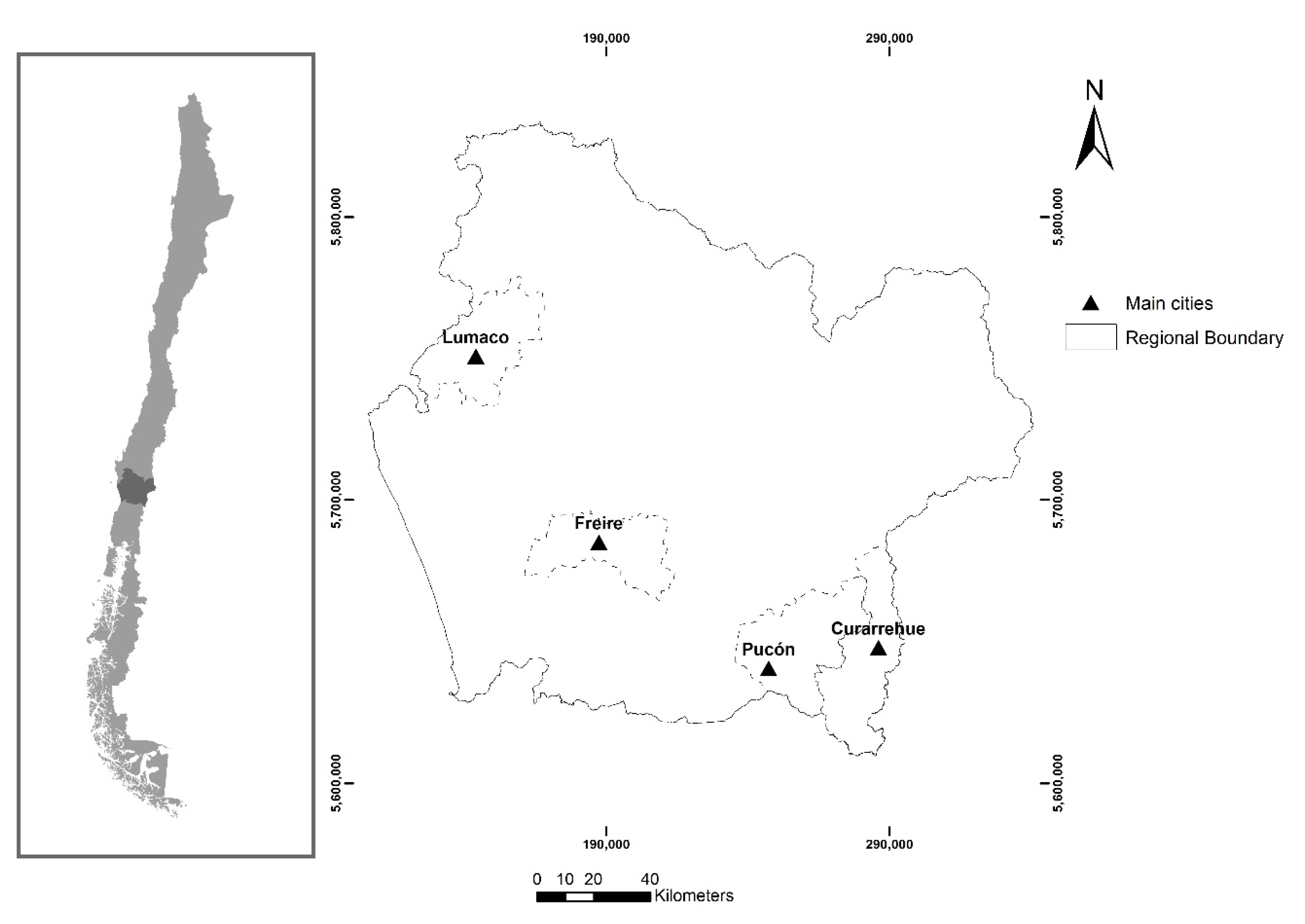
Our study site corresponds to the La Araucanía Region in south-central Chile, which covers an area of approximately 20,000 km². This region is included among the 35 global biodiversity hotspots [33,34] and, at local levels, has been promoted as a primary conservation target considering its high levels of species endemism and extinction threats [35]. In this region, we selected four landscapes: Freire, Lumaco, Pucón, and Curarrehue (Figure 1), which are similar in terms of their extension and biophysical characteristics, but different in terms of their main land-use and land-cover types and economic activities (

Table 1. Characteristics of four landscapes in the La Araucanía Region, south-central Chile.

	Freire	Lumaco	Pucón	Curarrehue
Location
Geomorphology	Central Valley	Coastal range	Pre-Andean range	Andean range
Area (km2)	90,268	110,684	123,944	116,460
Topography
Elevation (mean) (m) 1	130	350	800	1150
Slope (mean) (%) 1	2	10	15	20
Biophysical characteristics
Annual mean temperature (°C) 2	12.3	12.8	11.3	11.1
Annual precipitation (mm) 2	1539	1075	2238	1643
Climate	Temperate	Temperate	Temperate	Temperate
Socioeconomic
Population (inhabitants) 3	24,600	9500	28,500	7500
Main economic activities	Agriculture	Commercial plantations	Tourism	Livestock; tourism
Land cover types (%) 4
Native forest	17.3	22.2	61.2	65.4
Shrublands	6.2	10.9	11.2	16.9
Tree plantations	2.8	43.5	2.4	0.4
Agricultural lands	17.8	0.4	0.1	<0.1
Pastures and grasslands	55.2	23.0	13.9	10.1
Water bodies and wetlands	0.4	<0.1	7.3	0.4
Bare and impervious lands	0.3	0.1	3.6	6.4
Snow, ice, and other cover types	<0.1	0	0.4	0.4

¹ Global land Cover Facility (2018, http://www.landcover.org). ² Hijmans et al. 2005. ³ Censo de Población y Vivienda año 2017, Instituto Nacional de Estadísticas (INE). ⁴ Zhao et al. 2016.

). These areas represent a disturbance gradient which is rather representative of landscapes of south-central Chile where we find more conserved areas near to the Andean mountains.

Several empirical measures are used to assess landscape patterns, the simplest being composition indicators such as richness, diversity, land-cover proportion, and matrix identification. They are relevant general landscape descriptors of the disturbance degree. However, most landscape patterns stem from disturbances, where land use and land cover are the most relevant [36]. Therefore, the identification of land-use and land-cover patterns is a useful empirical measure to identify the degree of landscape disturbance. Some specific land covers (e.g., native forest) represent a clear indicator of naturalness or a low disturbance degree. Indicators such as the dominance of natural forest cover, deforestation rate, degradation, or regeneration have also been used as a proxy for naturalness or disturbance degree [37,38]. Other relevant land covers, particularly anthropic-induced ones, are the main drivers of land-use/cover change. A good example of this occurs in the Chilean global biodiversity hotspot where the area with the highest species richness of native forests has been mainly converted to exotic tree plantations [39]. In this context, we define a disturbance gradient according to the land-use type proportion in each landscape, decreasing in disturbance as described below.

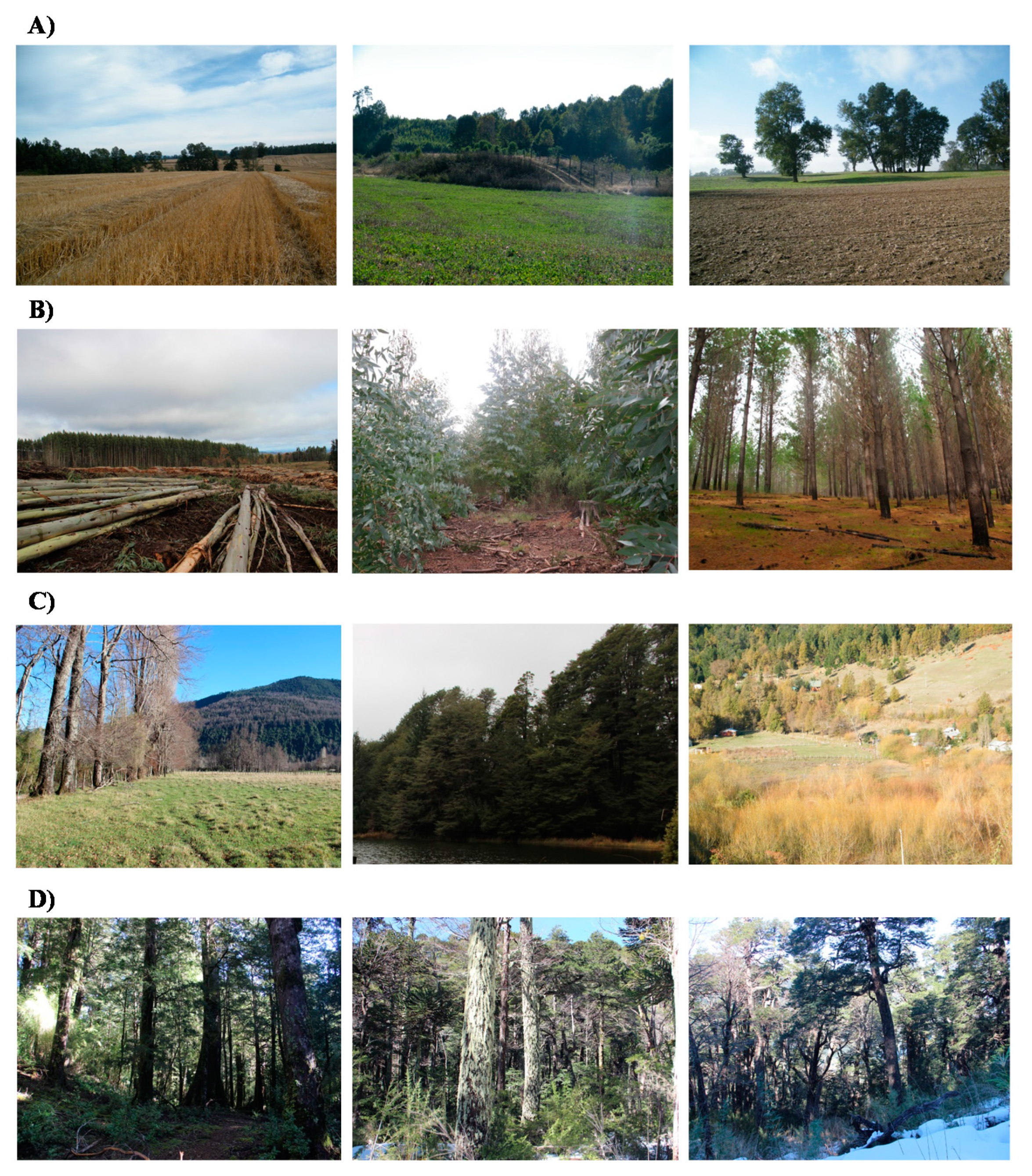
Freire is located in the Central Valley. Historical intensive agricultural activities have produced a high level of intervention in this landscape, where agricultural and pasturelands are the dominant land-use types (≈73%). Tree plantations represent a low proportion in the landscape (≈3%); however, Freire has the lowest proportion (≈17%) of native forests. Lumaco is located in the Coastal Range. It also presents a high level of human intervention mainly because the matrix of the landscape is represented by commercial forest plantations that occupy ≈43% of its area. When considering the area of agricultural land, the figure rises to ≈67% of the landscape. Pucón is located in the Pre-Andean Range, and its most important land-uses/covers are native forest (≈61%) and shrublands (≈11%). Here, the area of tree plantations and agricultural land is about 2% of the landscape, making it a municipality with a lower level of intervention. Its principal economic activity is tourism; hence, the high amount of native forest, which is popular among nature tourists. Curarrehue is the least disturbed landscape, located in the Andean Range. It is widely dominated by native forest (≈65%). Both tree plantations and agricultural land represent a small proportion of the landscape (<1%), having the lowest level of disturbance degree. The main economic activities are livestock farming and forestry as well as tourism.

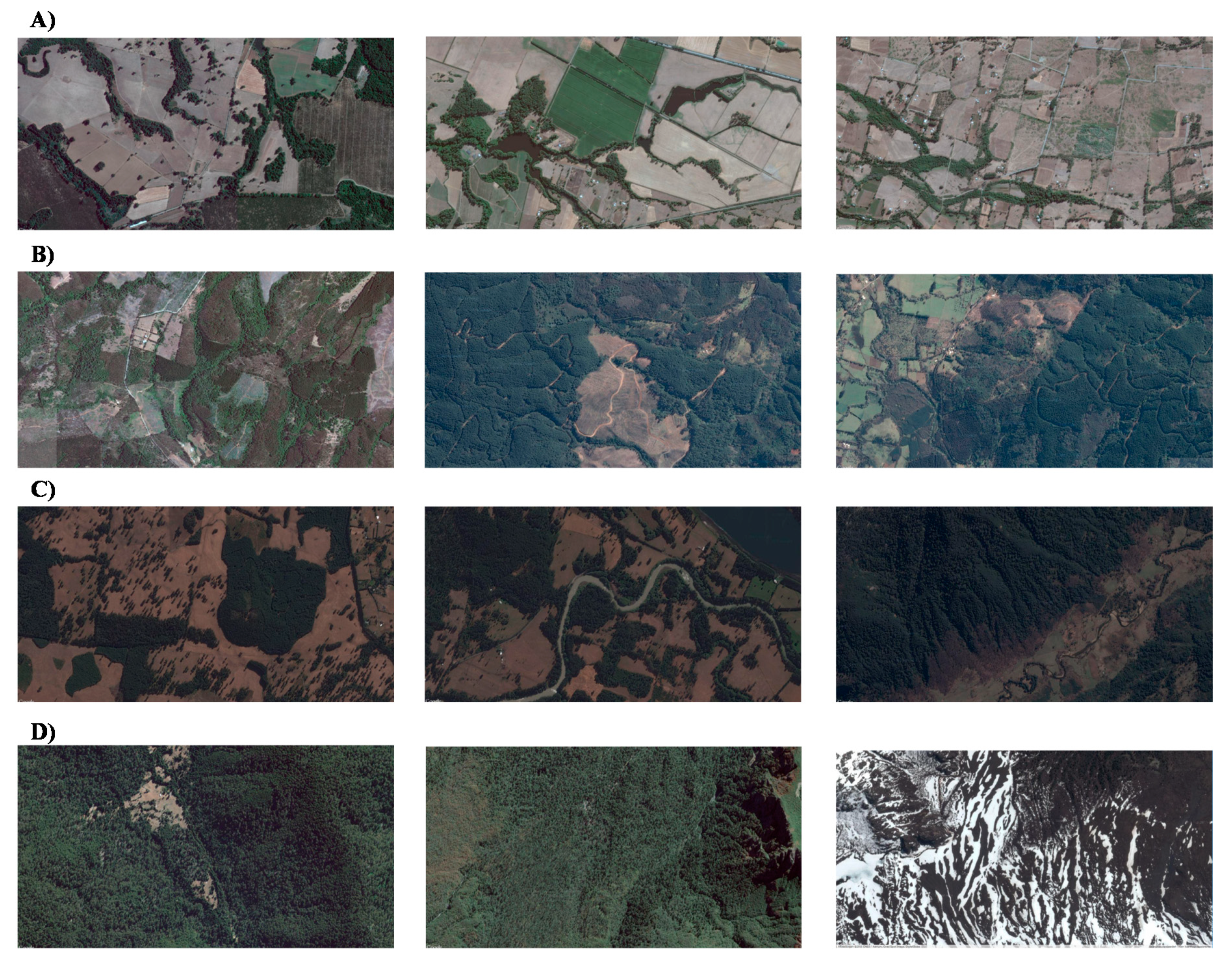
2.2. Type of Scene

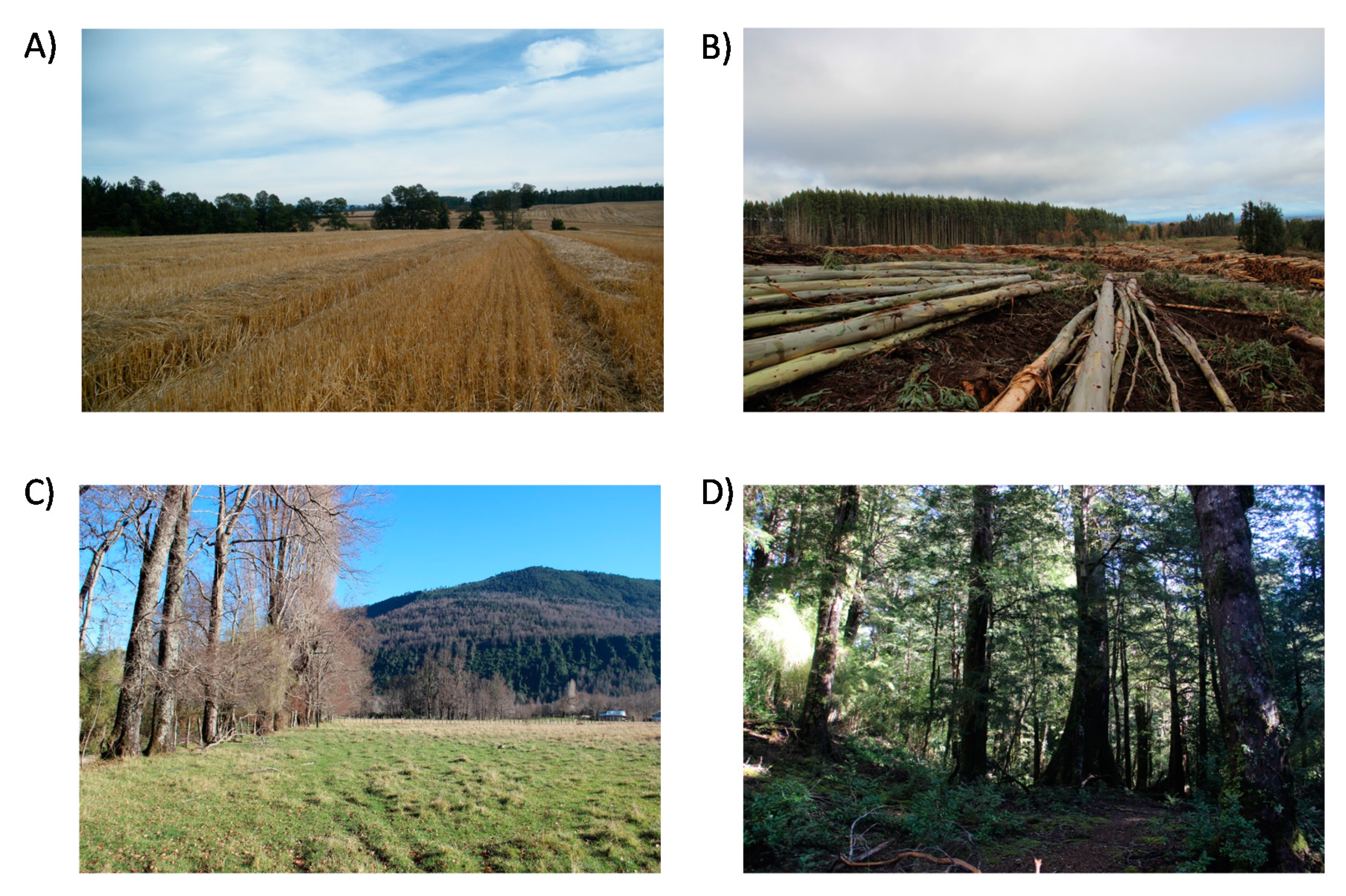
We used eye-level and aerial images (Figure 2). Eye-level images were taken during fieldwork using a conventional reflex digital camera. Over 100 images were available for our selection. The photographs were taken at eye-level on clear or less cloudy days, from about 10:00 a.m. to 4:00 p.m. to control for similar lighting conditions in mid-summer 2015, during which time the vegetation retained a relatively constant appearance. The images finally selected were aesthetically equal to each other; they were not influenced by the weather and represented the landscape with a certain amount of depth. If water and snow are typical for the landscape concerned, then they were represented in the chosen aerial images.

For aerial images, 50 sample points were taken from Google Earth with a scale of 1:10,000 in each landscape. From these 50 points, we selected images that represented the main landscape characteristics (i.e., its land-use/cover patterns). All images were captured in a window from 2010 to 2015 during spring and summer to guarantee that deciduous trees were not yet defoliated and had fully developed canopies. The final selection of images was made using a survey based on input from local experts, as suggested by Palmer and Hoffman [40]. Local experts were selected according to the following criteria: verified working on environmental topics and knowledge about the region. A total of 10 local experts were consulted to select the final eye-level and aerial images. Local experts selected three images for each type of landscape (Appendix A and Appendix B).

2.3. Survey on Landscape Preferences

To test responses to the different landscape preferences and perceptions, we used an online questionnaire. We used the KU Leuven web survey service to create the survey and conducted it through this platform. A cross-sectional correlational study was conducted on a non-probabilistic sample aimed at a general adult population. Our recruitment technique was a snowball strategy, a combination of professional and social networks, undergraduate and graduate students, and personal contacts, were invited to participate and share this invitation among their contacts. Participants had been informed of the nature of this study and marked their decision to participate voluntarily and anonymously. Furthermore, people from different faculties of the University of La Frontera were invited to answer the questionnaire in the computer lab. A researcher received them, explained the ethical and objective aspects of the study, and gave general instructions.

First, the survey collected demographic information about the respondent to determine whether the interviewees constituted a representative sample and to check for any significant correlations with landscape preferences and perceptions. The following social variables were further collected: gender, age, current professional activity, the current location of residence, time of residence, type of residence, and education level.

Second, we presented the participants with landscape images one at a time. We presented the selected three eye-level, and three aerial images of each of the four landscapes (24 images in total; Appendix A and Appendix B). Participants were not informed about which community the images came from. Images did not include any particular place or specific touristic point, and images were presented at random order to each respondent. We first presented the participant with the 12 eye-level images (Appendix A) and then the 12 aerial images (Appendix B). For each image, respondents were asked about the following preference and perception measures: preference for living in, preference for visiting, perceived scenic beauty, perceived well-being, perceived risk, and perceived disturbance degree. Each image was accompanied by some sentences related to the preference aspects (Appendix C).

We assessed the effect of a function of the setting as suggested in previous research [41,42], where preference was measured the same way, using the following sentences: “I like this place for living”, “I like this place for visiting”, “This place is nice”, “This place makes me feel good”, “This place makes me feel at risk”, and “This place is natural”. Given that preferences sometimes influence actions or decisions, it is essential to understand the steps that people can and should take as they express their preferences [43,44].

Among the measures of positive human response to landscapes, personal judgments of aesthetic and scenic beauty have been most frequently used [45,46]. Preference is also understood as the initial response to an environment that has developed through human evolution [47,48] and thus, to whether an environment can support human survival and well-being [49]. One classical approach in landscape preference studies assumes that this appreciation reflects on how well the given environments support sufficient well-being [50]. Most of these studies emphasize the physical characteristics of restorative and preferred environments [21]. To survive, human responses to environments, based primarily on the differentiation of habitable from inhabitable settings, must be motivationally robust [47]. Some empirical research has concluded that to plan landscapes, it is necessary to incorporate amenities and risk reduction [51]. Moreover, the inclusion of perceived risk measures helps to understand the innate human needs for protective spaces (refuge) and perceptions of safety and danger because these are relevant landscape attributes [52,53]. Finally, the degree of wilderness (e.g., the presence of well-preserved human-made elements, the percentage of plant cover, the amount of water, the presence of mountains) may be a factor contributing to the overall visual preference [10]. Thus, we included a measure of the perceived disturbance degree for different landscapes to compare and validate experts’ and lay people’s judgments.

The specific questions for each preference aspect are detailed in Appendix C. These questions were the same for each image. The questions were asked in three different ways. For the first three questions (a–c), we used a seven-point Likert scale to ask the respondent their agreement level with each sentence, with one being “completely disagree” and seven “completely agree”. For the second three questions (d–f), we used a semantic differential scale with opposite adjectives at both ends [54]. This required subjects to rate whether the image agreed with one of the two opposite adjectives. The scale contained “neutral” in the middle and “a little bit”, “a lot”, and “too much” on the two sides. The bipolar adjectives were considered with the same seven-point Likert scale with bipolar values like the previous questions.

We collected responses from October 2015 to February 2016. It was done by sharing the survey on social media and by organizing meetings with people. The time needed to complete the survey was 40 min. Beforehand, the participants were asked to sign an agreement stating the risks and conditions of the survey.

2.4. Data Analysis

We first checked for normal distribution of perception values, running 1000 iterations of Shapiro tests using 30-data samplings. We also checked for mean and median values in the histogram. Data showed a normal distribution. We tested differences between image types (i.e., eye-level and aerial) and perceptions (i.e., the six questions) using a two-way ANOVA. When necessary, we then used Tukey’s HSD post hoc comparisons to evaluate interaction terms, which have higher power and are readily available in many statistics packages. Furthermore, to analyze potential relationships between perceptions on the different landscapes and image types, we used a two-way randomized block ANOVA, in which we included landscape and image types as fixed factors and the questions as blocks.

To explore potential relationships between perceptions and the disturbance level of the landscapes, we built multiple correlation matrices for each question and land-cover type. We included the percentage cover of four individual cover types (i.e., native forest, tree plantation, croplands, grasslands) and six cover type combinations representing natural and anthropic land uses: (1) native vegetation (native forest + shrublands); (2) forested areas (native forest + tree plantations); (3) agriculture (croplands + pastures); (4) anthropic areas (croplands + pastures + tree plantation); (5) native forest importance (proportion of native forest from the total forested area); and (6) forested area importance (proportion of forested areas from the total landscape extent, including both native and non-native forests). Finally, we described the relationships between the preference and perception values concerning the cover types selected by correlation tests.

3. Results

We collected a total of 107 responses through the online survey, and all participants answered all questions. There were 52 females (49%) with an average age of 27 years old (SD = 8.03); and 55 male respondents (51%) with an average age of 27 years old (SD = 7.2). There were 86 participants (80%) from Temuco, 9 (8%) lived in other locations of the Araucanía Region, 12 participants (11%) lived in another Chilean region (Santiago, Talca, Chillán and Osorno), or country (Venezuela, Colombia, Mexico, and Spain), and 13 respondents (12%) identified as having a Mapuche ethnic background. Also, 53 participants were students (50%), 47 were employed (44%), and 7 participants did not work or study at the time of the survey (7%). There were 88 participants (82%) with a university or a graduate degree, and 19 participants (18%) had a technical degree or lower. Additionally, 92 participants (86%) lived in the urban zone, 10 (9%) in the rural zone, and 5 participants (5%) lived in a semi-rural zone. At least 14 participants have lived in the region for less than a year (13%), 17 for 1–5 years (16%), another 17 for 5–10 years (16%), and 59 for more than 10 years (55%). The tests to assess the influence of these variables in the perceptions/preferences mostly showed no significant influence.

3.1. Landscape Preferences and Perceptions

Perceptions varied in terms of the dimension evaluated and the type of image used (

Table 2. Randomized Block ANOVA comparing image types and landscapes for six preference questions (blocks).

	df	Sum Square	Mean Square	F-Value	Pr(>F)
Image type	1	120	119.9	46.62	<0.0001
Landscape	3	633	210.9	81.99	<0.0001
Question	5	1913	382.7	148.75	<0.0001
Image type: Landscape	3	282	94.1	36.6	<0.0001
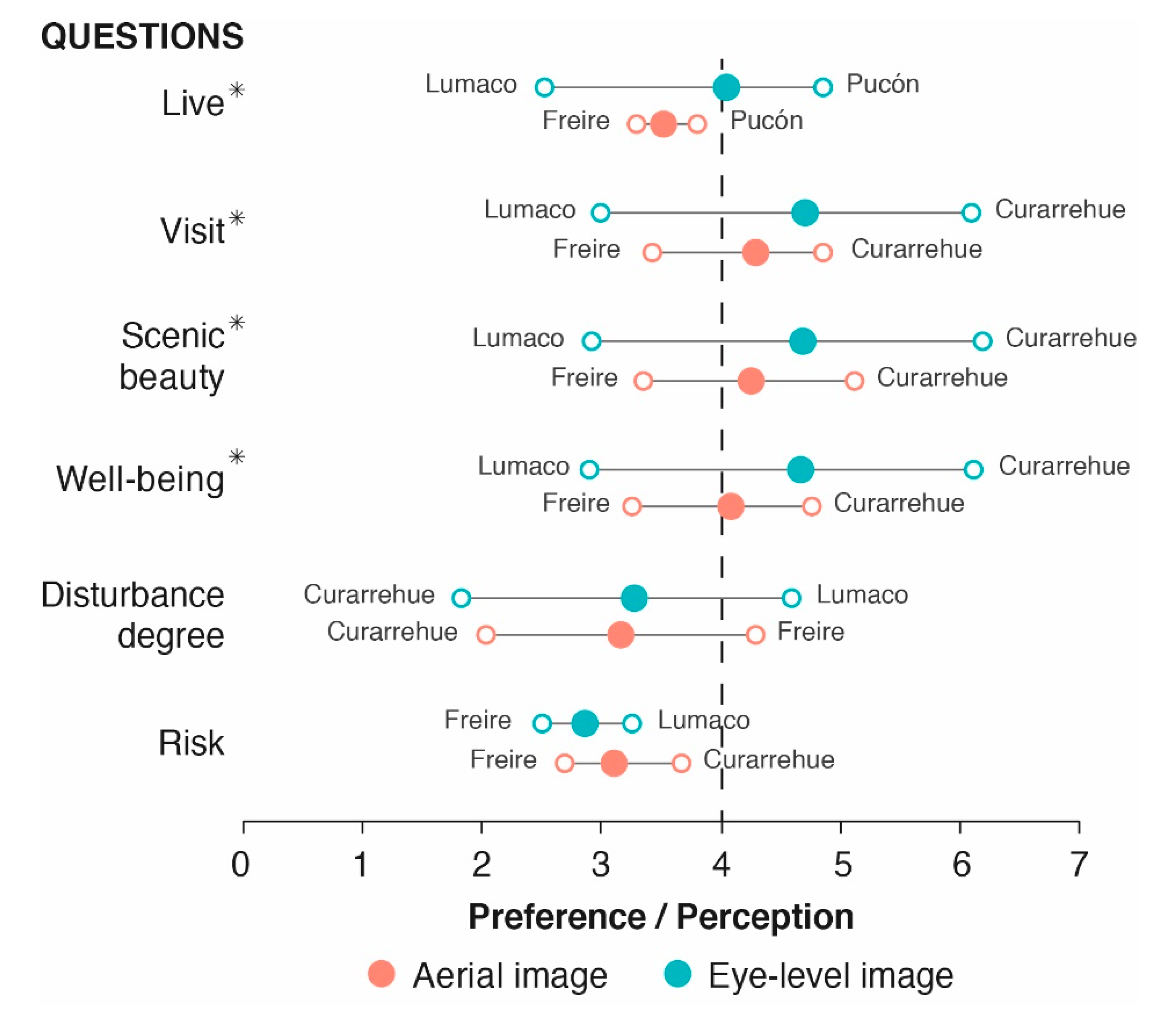
Residuals	5123	13,179	2.6

). In all dimensions (except for risk perception), some landscapes were perceived below the median value, while others were rated above it (Figure 3). In terms of absolute values, perception resulted to be different among locations (F = 129.51; p < 0.001), and among questions (F = 137.21; p < 0.001). Perception values for living, visiting, beauty, and well-being were higher than for risk and disturbance, suggesting that people tend to perceive these four landscapes more positively based on aesthetic features rather than perceiving them as unsafe or unpleasant.

Perceptions of scenic beauty, well-being, and visiting the landscape showed a similar pattern (Figure 3): the highest values for Curarrehue and the lowest for Lumaco when using eye-level images, but Curarrehue and Freire respectively when using aerial images. Perception for living was also the lowest for Lumaco and Freire when using eye-level and aerial images, respectively, but the highest for Pucón in both cases. Interestingly, when asked about risk and disturbance, Freire and Curarrehue were considered the best (lowest values), respectively, when using both image types. In contrast, Lumaco was considered the worst (highest values) and Curarrehue and Freire the best (lowest values), respectively, when using eye-level and aerial images.

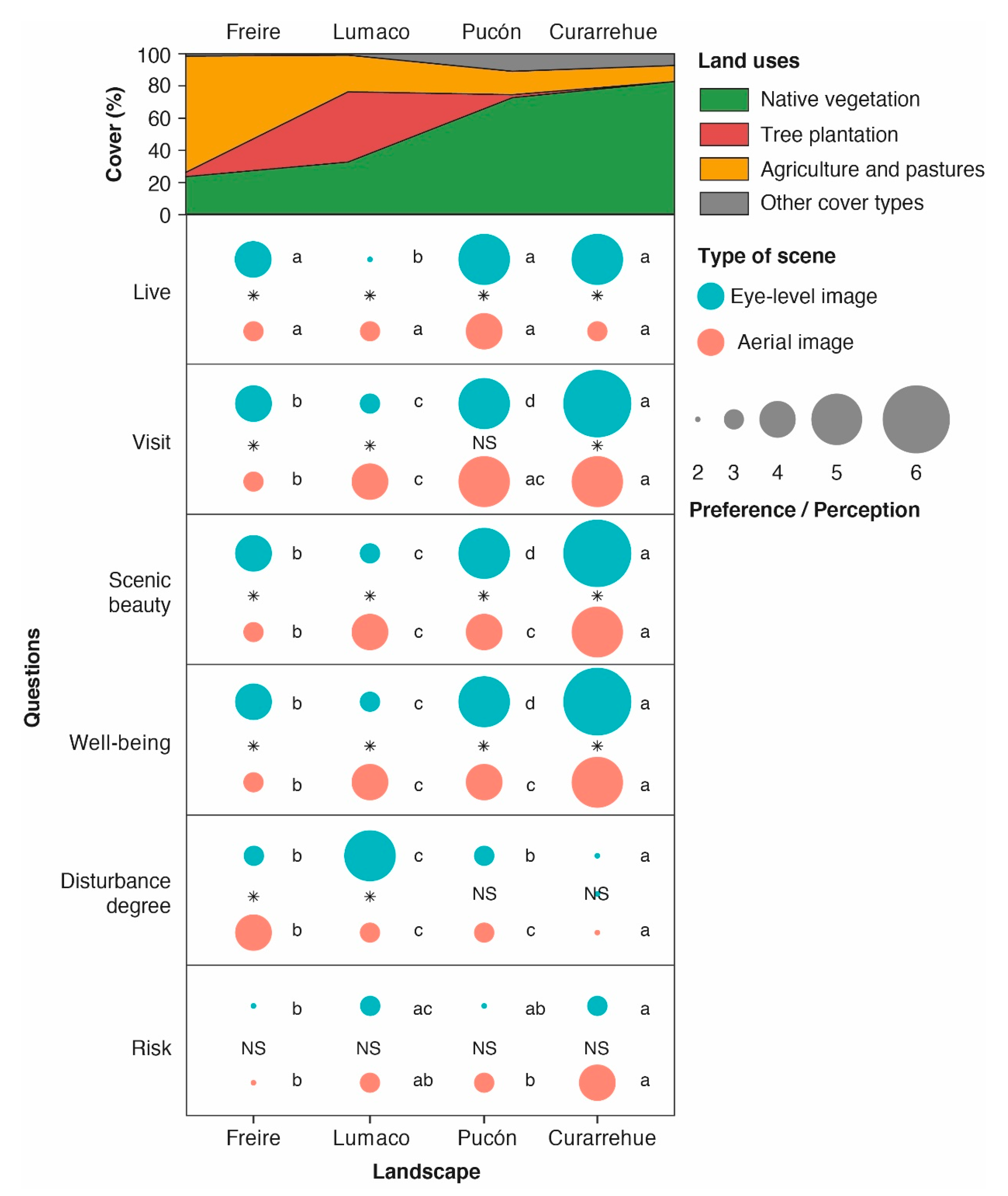
Overall, we observed a negative association between landscape preferences and perceptions and the landscape disturbance gradient (Figure 4; Appendix E). Landscapes with lower human intervention showed higher preferences by respondents and vice versa. This pattern is clearly observed for preferences for visiting, perceived scenic beauty and well-being, where there were significant differences between all landscapes. Likewise, the pattern is also observed in the preference for living, where we found marked differences among disturbed and conserved landscapes, but Pucón showed a higher but similar preference for living compared to Curarrehue. However, differences between these two landscapes, which have the lowest disturbance degree values, were non-significant. By contrast, the perceived risk showed an opposite pattern to the other preferences. The perceived risk was higher at both extremes of the gradient, the highest and the lowest disturbed landscapes, although there were no significant differences between these two landscapes. Low perceived risk was observed in the medium human-intervened landscapes, and no significant differences between these landscapes were found.

The results of multiple correlations supported these patterns. Preferences (for living in and visiting) and positive perceptions (beauty, well-being) were directly associated with native forested areas, and inversely with anthropic land uses (i.e., agriculture, pastures, and tree plantations) when using eye-level images (Appendix F). People significantly prefer and perceive better those landscapes with a higher proportion of the native forest cover, being all r² significant and varying between 0.50 and 0.62. However, the perception of this pattern was not evident when using aerial images, being all r² < 0.12, and the patterns were even less evident for negative perceptions (disturbance degree and risk). The disturbance degree was inversely associated with native vegetation covers when using both image types (r² = −0.48 and −0.43 for eye-level and aerial images, respectively). Interestingly, perceived risk showed a low correlation with land-use covers (r² < 0.18 for all land uses).

3.2. Type of Scene

Most preference and perception values were different for the comparison between eye-level and aerial images for each landscape (Figure 4; Appendix E). Changes in the preferences and perceptions showed similar patterns for all landscapes except Lumaco. In all cases, the “positive” perceptions (i.e., living, visiting, scenic beauty, and well-being) decreased when aerial images were used (p < 0.01; Figure 3). However, the “negative” perceptions (i.e., disturbance degree and risk) increased in Freire but not in Curarrehue and Pucón. Similarly but with an opposite pattern, Lumaco showed an increase in all preference values except the perceived disturbance degree, which increased, while the perceived risk did not change.

When using aerial images, the perceived landscape disturbance was consistent with the landscape disturbance gradient based on empirical attributes of landscapes, but not when using eye-level ones (Figure 4). When using eye-level images, Lumaco (and not Freire) was perceived as the landscape most disturbed, consistently with our correlation analyses, which showed that the tree plantation cover explained the perceived disturbance when using such images, but not when using aerial ones (Appendix F).

4. Discussion

Our results show that when assessing landscape preferences and perceptions based on images, using eye-level images or aerial images can produce different results. Although eye-level images tend to reveal preferences and perceptions more strongly than aerial images, the latter ones are more correlated to human intervention than eye-level images. The use of aerial images allows the perception of a larger area and the level of human intervention more accurately. Less human intervention is correlated to more preference for living in, visiting, scenic beauty, well-being, and risk level. We discuss below the implications of these results on land planning.

4.1. Landscape Preferences and Perceptions

Overall, landscape preferences and perceptions coincided with the disturbance gradient when using aerial images. People significantly prefer and perceive better those landscapes with greater native vegetation cover extent. Prior studies have suggested that the exposure to less disturbed and more “natural” environments (with higher tree cover), may be associated with greater stress reduction [55,56,57,58], affective restoration—including improvement in mood [59], enhancing people’s ability to focus their attention [60,61], and increasing the strength of neighborhood social ties [62]. Landscape preference studies have consistently found strong preferences for natural areas by both urban and rural dwellers [63]. Naturalness was consistently found to be a reliable predictor for people’s preferences, which was explained by the theory of evolution [19]. Nevertheless, despite this, we detected some contradictions: we found that landscapes less disturbed scored a higher risk and that the perceived risk also increased when using aerial images. Preferences and perceptions related to visiting and living resulted similarly, because people prefer the most conserved landscape in terms of visiting but not living in. Natural environments may contain several potential hazards, such as dangerous animals, unseen obstacles, or offenders in hiding, and the prediction of these dangers along with worries of getting lost may evoke a sense of fear [64]. Trees are widely recognized to provide multiple benefits, but they may sometimes be perceived as a burden [28], so the sense of safety (or conversely, perceived risk) may remain a consistent predictor of landscape preference [65]. Human factors such as gender or age could be predictors of the sense of safety; people with deeper connections to nature may be expected to feel safer [66].

Here we used a group comparison mostly referring to a single set of landscape images and focusing on familiarity and social construction by comparing differences among landscapes with similar spatial, cultural, and ecological attributes but varying percentage levels of native forest cover. It is possible, however, that a slight difference in environmental attributes may have impacted preference. A landscape is about a vaguely bounded area as a whole; thus, the aesthetic experience of the landscape requires that we consider the whole place. We might be attracted to details or particular features, but the feeling of the whole is our focus [67]. Few studies have analyzed how several or particular landscape features (e.g., native forest cover, land-use diversity, presence of livestock) may contribute specifically to these preferences, but see [68]. Future research should include specific landscape features related to the sociocultural background characteristics of the respondents. For instance, most of our respondents (92%) were from urban areas; therefore, we should explore the effect of the respondents’ territorial origin on their landscape preferences and perceptions. Further research may analyze demographic issues deeply. For instance, we found some gender-specific outcomes in environmental preferences [69]. Men scored the eye-level images of Pucón and Freire for the variable “disturbance degree” higher than women did, while women scored higher for the variable “preference to live”, “beauty” and, “perceived well-being”.

4.2. Type of Scene

Our most remarkable result is that assessment of landscape preferences is strongly affected by the type of images used. All preference values varied in most municipalities when image types were considered. When using aerial images, we found a match between the perceived and empirical measures of the landscape disturbance, but not when using the traditional eye-level images. Therefore, disturbance gradients may be masked when valuing landscape through eye-level images. In particular, the landscape most disturbed in terms of empirical measures (Freire) is perceived as the most disturbed when using aerial but not eye-level images. In this last case, Lumaco was perceived as the landscape with the highest disturbance degree, mainly due to its high cover of tree plantations, which is not perceived by people as a disturbance or risk. Identifying these classes at larger scales is problematic due to the current remote sensing techniques [70]. Therefore, people do not distinguish between plantations and native forests since these specific features can only be detected by people with some expertise in remote sensing visual analysis, so people just see green areas. This reason also explains how the overall preferences and perceptions are higher when using eye-level rather than aerial images. At the same time, Curarrehue was considered the least disturbed landscape, but also the highest risk when using aerial images, which is associated with the greenness that is of particular note in such images, reinforcing the idea that people may perceive fairly natural environments as potentially risky [64]. By contrast, Freire was considered the lowest risk landscape, but also the most disturbed when using aerial images, which is mainly associated with its dominant agricultural landscape matrix.

Implications of these results are relevant because, by far, most landscape preference studies use traditional eye-level images [11,17,18,22,23,24,25], and few studies have specifically assessed the impact of the type of scene on landscape preferences and perceptions, but see [29,30]. As our results show this type of image offers several advantages (free availability, easy to use, spatial resolution) but is not suitable for the assessment of some preferences (e.g., scenic beauty). However, Andrew et al. [71] point out that increased incorporation of the current generation of remotely sensed data products into ecosystem services assessments (e.g., cultural services which are closely linked to landscape preferences) can help drive a shift from reliance on simple proxies of ecosystem services to a more empirical focus.

Objective measures of the landscape such as texture, disturbance, or naturalness can be obtained using satellite images. An important point is that more abstract data sets like satellite images are more homogeneously assessed because personal factors that influence individual preferences are less critical [29]. Therefore, considering some specific preferences might not be appreciated when these traditional images are used, both types of images are useful to evaluate landscape preferences and perceptions better.

4.3. Implications for Landscape Management and Land Planning

Assessing the local natural landscape through the combination of eye-level and aerial images results in a useful tool to understand the relationship between people and their physical environment. Understanding how different approaches (i.e., type of scene) may be associated with different perceptions of landscape disturbance may help to evaluate people’s expectations for decisions on land planning and eventually consider in the decision-making process. Based on this resource, it is possible to make more informed judgments, improve the quality of environmental assessments in order to better plan and manage land and protection decisions [72]. Moreover, our results reveal that the use of traditional eye-level images (photographs) or aerial images (satellite) has enormous implications on landscape preferences and perceptions. The landscape disturbance gradient coincided with a decrease in the preference when using aerial images in terms of empirical measures. However, it was masked when valuing landscape through eye-level images, mainly due to people identifying non-native forested areas as anthropic in the latter case. In this light, we conclude that different types of scenes should be considered in order to embrace everyone’s landscape preferences and perceptions. It would make it possible to capture the whole picture, which is especially relevant for decision-making in landscape planning. Our findings can be useful for the design, management, and participatory planning of landscape, in which the different groups involved are often consulted. Some municipalities as Pucón have intense urbanization pressure in the last years, which is reflected in the increased urban area and derived conflicts [73]. Curarrehue has similar amenities as Pucón (e.g., naturalness, hot springs, snow) and connectivity has increased in the last years. So, urgently, some regulations and participatory planning should be considered for the near future of this municipality. A different conflict appears in Lumaco where exotic tree plantations dominate the landscape [74] and have helped the increase of forest fires in recent times and other undesirable effects [75]. So, in this area landscape planning focused on land-use management and other practices can be addressed to reduce forest fires. Lastly, Freire, as a dominant agricultural matrix, has great opportunities to improve landscape connectivity and combine production activities and conservation through landscape restoration. This type of landscape has important areas not used for agricultural production which can be restored through the planning buffer strips and hedgerow networks [76].

5. Conclusions

People’s preferences and perceptions are not neutral to the landscape disturbance gradient, but this relationship strongly depends on the type of scene used. A landscape disturbance gradient may be consistent with a decrease in preference when valuing the landscape using aerial images, but not through eye-level images. Eye-level images (and not aerial ones) appear to be more evident to evincing non-native forested areas to people. For decision-making on landscape planning, different scene types should be used, in order to embrace the landscape preferences and perceptions of all those involved. Current remote sensing data can help to better landscape assessments, in particular cultural ecosystems services, which are more related to landscape preferences. Our findings offer an opportunity for the design, management, and participatory planning of landscapes subjected to different human pressure, in which the different groups involved are often consulted to improve the provision of multiple ecosystem services.

References

1. Bieling, C.; Plieninger, T.; Pirker, H.; Vogl, C.R. Linkages between landscapes and human well-being: An empirical exploration with short interviews. Ecol. Econ. 2014, 105, 19–30. [Google Scholar] [CrossRef] [Green Version]
2. Council of Europe. Landscape Convention. Contribution to Human Rights, Democracy and Sustainable Development; Council of Europe Publishing: Strasbourg, France, 2018. [Google Scholar]
3. Selman, P. Sustainable Landscape Planning: The Reconnection Agenda; Taylor and Francis: Oxford, UK, 2012. [Google Scholar]
4. Van den Berg, A.E.; van Winsum-Westra, M. Manicured, romantic, or wild? The relation between need for structure and preferences for garden styles. Urban For. Urban Green. 2010, 9, 179–186. [Google Scholar] [CrossRef]
5. Bastian, O.; Stein, C.; Lupp, G.; Behrens, J.; Renner, C.; Grunewald, K. The appreciation of nature and landscape by tourism service providers and visitors in the Ore Mountains (Germany). Landsc. Online 2015, 41, 1–23. [Google Scholar] [CrossRef] [Green Version]
6. Millenium Ecosystem Assesment. Ecosystems and Human Well-Being: Synthesis; Island Press: Washington, DC, USA, 2005. [Google Scholar]
7. Schröter, M.; van der Zanden, E.H.; van Oudenhoven, A.P.E.; Remme, R.P.; Serna-Chavez, H.M.; de Groot, R.S.; Opdam, P. Ecosystem services as a contested concept: A synthesis of critique and counter-arguments. Conser. Lett. 2014, 7, 514–523. [Google Scholar] [CrossRef] [Green Version]
8. Fedele, G.; Locatelli, B.; Djoudi, H. Mechanisms mediating the contribution of ecosystem services to human well-being and resilience. Ecosyst. Serv. 2017, 28, 43–54. [Google Scholar] [CrossRef]
9. Arnberger, A.; Eder, R. Exploring the heterogeneity of cultural landscape preferences: A visual-based latent class approach. Landsc. Res. 2011, 36, 19–40. [Google Scholar] [CrossRef]
10. Arriaza, M.; Cañas-Ortega, J.F.; Cañas-Madueño, J.A.; Ruiz-Aviles, P. Assessing the visual quality of rural landscapes. Landsc. Urban Plan. 2004, 69, 115–125. [Google Scholar] [CrossRef]
11. De La Fuente De Val, G.; Mühlhauser, S.H. Visual quality: An examination of a south American mediterranean landscape, andean foothills east of Santiago (Chile). Urban For. Urban Green. 2014, 13, 261–271. [Google Scholar] [CrossRef]
12. Adevi, A.A.; Grahn, P. Preferences for landscapes: A matter of cultural determinants or innate reflexes that point to our evolutionary background? Landsc. Res. 2012, 37, 27–49. [Google Scholar] [CrossRef]
13. Byoung, E.; Kaplan, R. The perception of landscape style: A cross-cultural comparison. Landsc. Urban Plan. 1990, 19, 251–262. [Google Scholar] [CrossRef] [Green Version]
14. Múgica, M.; De Lucio, J.V. The role of on-site experience on landscape preferences. A case study at Doñana National Park (Spain). J. Environ. Manag. 1996, 47, 229–239. [Google Scholar] [CrossRef]
15. Langemeyer, J.; Baró, F.; Roebeling, P.; Gómez-Baggethun, E. Contrasting values of cultural ecosystem services in urban areas: The case of park Montjuïc in Barcelona. Ecosyst. Serv. 2015, 12, 178–186. [Google Scholar] [CrossRef]
16. Nijhuis, S.; Van Lammeren, R.; van der Hoeven, F. Exploring the Visual Landscape: Advances in Physiognomic Landscape Research in the Netherlands; IOS Press: Amsterdam, The Netherlands, 2011; Volume 2. [Google Scholar]
17. Dramstad, W.E.; Tveit, M.S.; Fjellstad, W.J.; Fry, G.L.A. Relationships between visual landscape preferences and map-based indicators of landscape structure. Landsc. Urban Plan. 2006, 78, 465–474. [Google Scholar] [CrossRef]
18. Kothencz, G.; Blaschke, T. Urban parks: Visitors’ perceptions versus spatial indicators. Land Use Policy 2017, 64, 233–244. [Google Scholar] [CrossRef]
19. Sevenant, M.; Antrop, M. The use of latent classes to identify individual differences in the importance of landscape dimensions for aesthetic preference. Land Use Policy 2010, 27, 827–842. [Google Scholar] [CrossRef]
20. Stamps, A.E. Use of photographs to simulate environments: A meta-analysis. Percept. Motor Ski. 1990, 71, 907–913. [Google Scholar] [CrossRef]
21. Scopelliti, M.; Carrus, G.; Bonaiuto, M. Is it really nature that restores people? A comparison with historical sites with high restorative potential. Front. Psychol. 2019, 9, 1–12. [Google Scholar] [CrossRef] [Green Version]
22. Berman, M.G.; Hout, M.C.; Kardan, O.; Hunter, M.C.R.; Yourganov, G.; Henderson, J.M.; Hanayik, T.; Karimi, H.; Jonides, J. The perception of naturalness correlates with low-level visual Features of environmental scenes. PLoS ONE 2014, 9, e114572. [Google Scholar] [CrossRef] [Green Version]
23. Kalivoda, O.; Vojar, J.; Skřivanová, Z.; Zahradník, D. Consensus in landscape preference judgments: The effects of landscape visual aesthetic quality and respondents’ characteristics. J. Environ. Manag. 2014, 137, 36–44. [Google Scholar] [CrossRef]
24. López-Martínez, F. Visual landscape preferences in Mediterranean areas and their socio-demographic influences. Ecol. Eng. 2017, 104, 205–215. [Google Scholar] [CrossRef]
25. Wang, R.; Zhao, J.; Liu, Z. Consensus in visual preferences: The effects of aesthetic quality and landscape types. Urban For. Urban Green. 2016, 20, 210–217. [Google Scholar] [CrossRef]
26. De Jong, K.; Albin, M.; Skärbäck, E.; Grahn, P.; Wadbro, J.; Merlo, J.; Björk, J. Area-aggregated assessments of perceived environmental attributes may overcome single-source bias in studies of green environments and health: Results from a cross-sectional survey in southern Sweden. Environ. Health 2011, 10, 4. [Google Scholar] [CrossRef] [PubMed] [Green Version]
27. Leslie, E.; Sugiyama, T.; Ierodiaconou, D.; Kremer, P. Perceived and objectively measured greenness of neighbourhoods: Are they measuring the same thing? Landsc. Urban Plan. 2010, 95, 28–33. [Google Scholar] [CrossRef]
28. Jiang, B.; Larsen, L.; Deal, B.; Sullivan, W.C. A dose-response curve describing the relationship between tree cover density and landscape preference. Landsc. Urban Plan. 2015, 139, 16–25. [Google Scholar] [CrossRef]
29. Frank, S.; Fürst, C.; Koschke, L.; Witt, A.; Makeschin, F. Assessment of landscape aesthetics—Validation of a landscape metrics-based assessment by visual estimation of the scenic beauty. Ecol. Indic. 2013, 32, 222–231. [Google Scholar] [CrossRef]
30. Ozkan, U.Y. Assessment of visual landscape quality using IKONOS imagery. Environ. Monit. Assess. 2014, 186, 4067–4080. [Google Scholar] [CrossRef]
31. Barroso, F.L.; Pinto-Correia, T.; Ramos, I.L.; Surová, D.; Menezes, H. Dealing with landscape fuzziness in user preference studies: Photo-based questionnaires in the Mediterranean context. Landsc. Urban Plan. 2012, 104, 329–342. [Google Scholar] [CrossRef] [Green Version]
32. LALI. La Iniciativa Latinoamericana del Paisaje; LALI: Cund, Colombia, 2012. [Google Scholar]
33. Mittermeier, R.A.; Turner, W.R.; Larsen, F.W.; Brooks, T.M.; Gascon, C. Global biodiversity conservation: The critical role of hotspots. In Biodiversity Hotspots; Springer: Berlin/Heidelberg, Germany, 2011; pp. 3–22. [Google Scholar] [CrossRef]
34. Myers, N.; Mittermeier, R.A.; Mittermeier, C.G.; da Fonseca, G.A.B.; Kent, J. Biodiversity hotspots for conservation priorities. Nature 2000, 403, 853–858. [Google Scholar] [CrossRef]
35. Smith-Ramírez, C. The Chilean coastal range: A vanishing center of biodiversity and endemism in South American temperate rainforests. Biodivers. Conserv. 2004, 13, 373–393. [Google Scholar] [CrossRef]
36. Turner, M.; Gardner, R.; O’Neill, R. Landscape Ecology in Theory and Practice. Patterns and Process; Springer: New York, NY, USA, 2001. [Google Scholar]
37. Sengl, P.; Magnes, M.; Erdos, L.; Berg, C. A test of naturalness indicator values to evaluate success in grassland restoration. Commun. Ecol. 2017, 18, 184–192. [Google Scholar] [CrossRef]
38. Sylvester, S.P.; Heitkamp, F.; Sylvester, M.D.P.V.; Jungkunst, H.F.; Sipman, H.J.M.; Toivonen, J.M.; Gonzales Inca, C.A.; Ospina, J.C.; Kessler, M. Relict high-Andean ecosystems challenge our concepts of naturalness and human impact. Sci. Rep. 2017, 7, 1–13. [Google Scholar] [CrossRef] [PubMed] [Green Version]
39. Miranda, A.; Altamirano, A.; Cayuela, L.; Lara, A.; González, M. Native forest loss in the Chilean biodiversity hotspot: Revealing the evidence. Reg. Environ. Chang. 2017, 17, 285–297. [Google Scholar] [CrossRef]
40. Palmer, J.F.; Hoffman, R.E. Rating reliability and representation validity in scenic landscape assessments. Landsc. Urban Plan. 2001, 54, 149–161. [Google Scholar] [CrossRef]
41. Peron, E.; Purcell, A.T.; Staats, H.; Falchero, S.; Lamb, R.J. Models of preference for outdoor scenes. Environ. Behav. 1998, 30, 282–305. [Google Scholar] [CrossRef]
42. Purcell, T.; Peron, E.; Berto, R. Why do preferences differ between scene types? Environ. Behav. 2001, 33, 93–106. [Google Scholar] [CrossRef]
43. Korpela, K.; Nummi, T.; Lipiäinen, L.; De Bloom, J.; Sianoja, M.; Pasanen, T.; Kinnunen, U. Nature exposure predicts well-being trajectory groups among employees across two years. J. Environ. Psychol. 2017, 52, 81–91. [Google Scholar] [CrossRef]
44. Van den Berg, A.E.; Koole, S.L. New wilderness in the Netherlands: An investigation of visual preferences for nature development landscapes. Landsc. Urban Plan. 2006, 78, 362–372. [Google Scholar] [CrossRef]
45. Florida, R.; Mellander, C.; Stolarick, K. Beautiful places: The role of perceived aesthetic beauty in community satisfaction. Reg. Stud. 2011, 45, 33–48. [Google Scholar] [CrossRef]
46. Hadavi, S.; Sullivan, W.C. Environmental aesthetics. In Handbook of Behavioural and Cognitive Geography; Montello, D.R., Ed.; Edward Elgar Publishing: Cheltenham, UK, 2018. [Google Scholar]
47. Han, K.T. Responses to six major terrestrial biomes in terms of scenic beauty, preference, and restorativeness. Environ. Behav. 2007, 39, 529–556. [Google Scholar] [CrossRef]
48. Russell, R.; Guerry, A.D.; Balvanera, P.; Gould, R.K.; Basurto, X.; Chan, K.M.A.; Klain, S.; Levine, J.; Tam, J. Humans and nature: How knowing and experiencing nature affect well-being. Annu. Rev. Environ. Resour. 2013, 38. [Google Scholar] [CrossRef]
49. Scopelliti, M.; Carrus, G.; Bonnes, M. Natural landscapes. In The Oxford Handbook of Environmental and Conservation Psychology; Oxford University Press: Oxford, UK, 2012; pp. 332–347. [Google Scholar]
50. Collado, S.; Staats, H.; Corraliza, J.A.; Hartig, T. Restorative environments and health. In International Handbooks of Quality-of-Life; Fleury-Bahi, G., Pol, E., Navarro, O., Eds.; Springer International Publishing: New York, NY, USA, 2017; pp. 127–148. [Google Scholar]
51. Gill, N.; Dun, O.; Brennan-Horley, C.; Eriksen, C. Landscape preferences, amenity, and bushfire risk in New South Wales, Australia. Environ. Manag. 2015, 56, 738–753. [Google Scholar] [CrossRef] [PubMed] [Green Version]
52. Eriksen, C.; Gill, N. Bushfire and everyday life: Examining the awareness-action “gap” in changing rural landscapes. Geoforum 2010, 41, 814–825. [Google Scholar] [CrossRef]
53. Jansson, M.; Fors, H.; Lindgren, T.; Wiström, B. Perceived personal safety in relation to urban woodland vegetation—A review. Urban For. Urban Green. 2013, 12, 127–133. [Google Scholar] [CrossRef] [Green Version]
54. Osgood, C.E.; Suci, G.J.; Tannenbaum, P.H. The Measurement of Meaning; University of Illinois Press: Champaign, IL, USA, 1957. [Google Scholar]
55. Beil, K.; Hanes, D. The influence of urban natural and built environments on physiological and psychological measures of stress—A pilot study. Int. J. Environ. Res. Public Health 2013, 10, 1250–1267. [Google Scholar] [CrossRef] [PubMed] [Green Version]
56. Roe, J.; Thompson, C.; Aspinall, P.; Brewer, M.; Duff, E.; Miller, D.; Mitchell, R.; Clow, A. Green space and stress: Evidence from cortisol measures in deprived urban communities. Int. J. Environ. Res. Public Health 2013, 10, 4086–4103. [Google Scholar] [CrossRef] [PubMed] [Green Version]
57. Tyrväinen, L.; Ojala, A.; Korpela, K.; Lanki, T.; Tsunetsugu, Y.; Kagawa, T. The influence of urban green environments on stress relief measures: A field experiment. J. Environ. Psychol. 2014, 38, 1–9. [Google Scholar] [CrossRef]
58. Ward Thompson, C.; Roe, J.; Aspinall, P.; Mitchell, R.; Clow, A.; Miller, D. More green space is linked to less stress in deprived communities: Evidence from salivary cortisol patterns. Landsc. Urban Plan. 2012, 105, 221–229. [Google Scholar] [CrossRef] [Green Version]
59. Van den Berg, A.E.; Koole, S.L.; van der Wulp, N.Y. Environmental preference and restoration: (How) are they related? J. Environ. Psychol. 2003, 23, 135–146. [Google Scholar] [CrossRef]
60. Berman, M.G.; Jonides, J.; Kaplan, S. The Cognitive Benefits of Interacting With Nature. Psychol. Sci. 2008, 19, 1207–1212. [Google Scholar] [CrossRef]
61. Kuo, F.E.; Faber Taylor, A. A Potential Natural Treatment for Attention-Deficit/Hyperactivity Disorder: Evidence From a National Study. Am. J. Public Health 2004, 94, 1580–1586. [Google Scholar] [CrossRef]
62. Holtan, M.T.; Dieterlen, S.L.; Sullivan, W.C. Social life under cover. Environ. Behav. 2015, 47, 502–525. [Google Scholar] [CrossRef]
63. Silverman, I.; Choi, J. Locating places. In The Handbook of Evolutionary Psychology; John Wiley & Sons, Inc.: Hoboken, NJ, USA, 2015; pp. 177–199. [Google Scholar] [CrossRef]
64. Andrews, M.; Gatersleben, B. Variations in perceptions of danger, fear and preference in a simulated natural environment. J. Environ. Psychol. 2010, 30, 473–481. [Google Scholar] [CrossRef] [Green Version]
65. Herzog, T.R.; Kutzli, G.E. Preference and perceived danger in field/forest settings. Environ. Behav. 2002, 34, 819–835. [Google Scholar] [CrossRef]
66. Tang, I.C.; Sullivan, W.C.; Chang, C.Y. Perceptual evaluation of natural landscapes: The role of the individual connection to nature. Environ. Behav. 2015, 47, 595–617. [Google Scholar] [CrossRef] [Green Version]
67. Brook, I. Aesthetic appreciation of landscape. In The Routledge Companion to Landscape Studies; Howard, P., Thompson, I., Waterton, E., Eds.; Taylor & Francis: Oxford, UK, 2013; pp. 108–118. [Google Scholar]
68. Van Zanten, B.T.; Zasada, I.; Koetse, M.J.; Ungaro, F.; Häfner, K.; Verburg, P.H. A comparative approach to assess the contribution of landscape features to aesthetic and recreational values in agricultural landscapes. Ecosyst. Serv. 2016, 17, 87–98. [Google Scholar] [CrossRef]
69. Rosa, C.D.; Larson, L.R.; Collado, S.; Cloutier, S.; Profice, C.C. Gender differences in connection to nature, outdoor preferences, and nature-based recreation among college students in Brazil and the United States. Leis. Sci. 2020, 1–21. [Google Scholar] [CrossRef]
70. Andrew, M.E.; Wulder, M.A.; Nelson, T.A. Potential contributions of remote sensing to ecosystem service assessments. Prog. Phys. Geogr. 2014, 38, 328–353. [Google Scholar] [CrossRef] [Green Version]
71. Potschin, M.; Haines-Young, R. Landscapes, sustainability and the place-based analysis of ecosystem services. Landsc. Ecol. 2013, 28, 1053–1065. [Google Scholar] [CrossRef]
72. Vergara, G.; Ibarra, J.T. Paisajes en transición: Gradientes urbano-rurales y antropización del bosque templado andino del sur de Chile. Rev. Geogr. Norte Grande 2019, 73, 93–111. [Google Scholar] [CrossRef] [Green Version]
73. Miranda, A.; Altamirano, A.; Cayuela, L.; Pincheira, F.; Lara, A. Different times, same story: Native forest loss and landscape homogenization in three physiographical areas of south-central of Chile. Appl. Geogr. 2015, 60, 20–28. [Google Scholar] [CrossRef]
74. Bowman, D.; Moreira-Munoz, A.; Kolden, C.A.; Chavez, R.O.; Munoz, A.A.; Salinas, F.; Gonzalez-Reyes, A.; Rocco, R.; de la Barrera, F.; Williamson, G.J.; et al. Human-environmental drivers and impacts of the globally extreme 2017 Chilean fires. Ambio 2019, 48, 350–362. [Google Scholar] [CrossRef] [PubMed]
75. Hansen, M.C.; Potapov, P.V.; Moore, M.; Hancher, M.; Turubanova, S.A.; Tyukavina, A.; Thau, D.; Stehman, S.V.; Goetz, S.J.; Loveland, T.R.; et al. High-resolution global maps of of 21st-century forest cover change. Science 2013, 850, 850–854. [Google Scholar] [CrossRef] [PubMed] [Green Version]
76. Rey Benayas, J.M.; Altamirano, A.; Miranda, A.; Catalan, G.; Prado, M.; Lisón, F.; Bullock, J. Landscape restoration in a mixed agricultural-forest catchment: Planning a buffer strip and hedgerow network in a Chilean biodiversity hotspot. Ambio 2020, 49, 310–323. [Google Scholar] [CrossRef] [PubMed] [Green Version]
Figure 1. Location of the four landscapes in the La Araucanía Region, south-central Chile.
Land 09 00306 g001
Figure 2. Examples of eye-level images used for four landscapes in the La Araucanía Region, south-central Chile: (A) Freire, (B) Lumaco, (C) Pucón, and (D) Curarrehue. See Appendix A and Appendix B for the full list of images.
Land 09 00306 g002
Figure 3. Minimum and maximum values (empty circles) for the perception for six questions on four landscapes in the La Araucanía Region using eye-level and aerial images. The name of the community with those values is showed beside the circles. For details on each question and image type, see the main text. Full circles show the mean value for the four landscapes. * p < 0.01 in Tukey’s post-hoc comparisons among the type of images.
Land 09 00306 g003
Figure 4. Mean score (Likert scale) of landscape preferences and perceptions using eye-level and aerial images for four landscapes of the La Araucanía Region, south-central Chile. n.s: not significant; * p < 0.01 for individual comparisons for each landscape in each question. For the exact values of the lower panel of the figure, see Appendix D. Different letters show significant differences (p < 0.05) in Tukey’s post-hoc comparisons in the interaction term of two-way ANOVAs for six questions on preference values for four landscapes using two image types (eye-level and aerial).
Land 09 00306 g004