The Economic Accessibility of CO₂ Sequestration through Bioenergy with Carbon Capture and Storage (BECCS) in the US

Abstract

Bioenergy with carbon capture and storage (BECCS) is one strategy to remove CO₂ from the atmosphere. To assess the potential scale and cost of CO₂ sequestration from BECCS in the US, this analysis models carbon sequestration net of supply chain emissions and costs of biomass production, delivery, power generation, and CO₂ capture and sequestration in saline formations. The analysis includes two biomass supply scenarios (near-term and long-term), two biomass logistics scenarios (conventional and pelletized), and two generation technologies (pulverized combustion and integrated gasification combined cycle). Results show marginal cost per tonne CO₂ (accounting for costs of electricity and CO₂ emissions of reference power generation scenarios) as a function of CO₂ sequestered (simulating capture of up to 90% of total CO₂ sequestration potential) and associated spatial distribution of resources and generation locations for the array of scenario options. Under a near-term scenario using up to 206 million tonnes per year of biomass, up to 181 million tonnes CO₂ can be sequestered annually at scenario-average costs ranging from $62 to $137 per tonne CO₂; under a long-term scenario using up to 740 million tonnes per year of biomass, up to 737 million tonnes CO₂ can be sequestered annually at scenario-average costs ranging from $42 to $92 per tonne CO₂. These estimates of CO₂ sequestration potential may be reduced if future competing demand reduces resource availability or may be increased if displaced emissions from conventional power sources are included. Results suggest there are large-scale opportunities to implement BECCS at moderate cost in the US, particularly in the Midwest, Plains States, and Texas.

1. Introduction

Bioenergy with carbon capture and storage (BECCS) combines bioenergy with geologic carbon capture and storage to produce power (typically electricity or potentially liquid fuels) while removing CO₂ from the atmosphere [1,2]. As demand for atmospheric CO₂ drawdown increases, negative-emissions technologies (NETs) for CO₂ such as BECCS may be an important component of overall strategies to reduce atmospheric CO₂ concentrations [3,4]. The extent to which the US bioeconomy can be employed to meet potential future carbon management goals through NETs will depend on the potential quantity and cost of CO₂ sequestration. To understand the national potential for BECCS in the US to contribute to these goals, here we quantify the potential cost and quantity of BECCS as influenced by biomass resources, supply chain and power generation configurations, and proximity to geological formations suitable for BECCS. The main output of this analysis is supply curves illustrating the potential supply and associated cost of CO₂ sequestration under a range of biomass resource, logistics, generation, and carbon accounting scenarios.

The Intergovernmental Panel on Climate Change (IPCC) [5] finds that “rapid and far-reaching” transitions in land management, energy production, and civil infrastructure are required to limit global warming to 1.5 °C. These can include reduced CO₂ emission from fossil energy, and increased CO₂ sequestration through afforestation, agricultural practices, and NETs, such as BECCS. The best approach to manage atmospheric CO₂ concentrations is subject to broad uncertainties (e.g., technology, economics, and the course of the global COVID-19 pandemic) and is unknown. Because of these uncertainties, the IPCC [5] presents multiple potential pathways to limit global warming to 1.5 °C or less. Three of these four pathways rely on BECCS to meet this goal. Of the four IPCC illustrative pathways to limit climate change, Pathways 2, 3, and 4 include 151, 414, and 1191 cumulative GtCO₂ removed via BECCS globally by 2100 ([5], Figure SPM.3b). The present analysis aims to understand the US potential (supply and cost) to contribute to carbon dioxide removal through BECCS.

Potential supply is a first key criterion of the feasibility of BECCS. The US has an untapped potential of about 750 to 1050 million tonnes of biomass per year, depending on offered price and future yields [6]. Employing these resources in the bioeconomy can reduce CO₂ emissions and contribute nearly $259 billion and 1.1 million jobs in the US [7]. Previous efforts have explored the potential to use US biomass resources for BECCS. Baik et al. [8] find that about 25% of these biomass resources are likely to be found over geological formations suitable for BECCS, and they estimate that the US has the potential to remove up to 110 and 630 million tonnes CO₂ per year, after accounting for biomass colocation with storage basins and injectivity (see Section 2.2). Other research has found that western North America has the potential to sequester ~150 million tonnes per year by 2050 [9], and that BECCS can capture 38 million tonnes CO₂ from current ethanol plants at costs <$90 per tonne CO₂ [10]. Building on these studies, the present analysis explores potential supplies of CO₂ sequestration through BECCS in the US.

A second key criterion in assessing the potential feasibility of BECCS is cost. Because of opportunity costs of capital, the cost of reducing atmospheric CO₂ is a challenge to meeting climate change targets. Costs of carbon capture, utilization, and storage (CCUS) are perceived to be high, and a holistic valuation of the supply chain is needed to understand the economic potential of CCS [11]. BECCS is broadly estimated to cost between $50 and $250 per tonne CO₂ sequestered in an assessment of thirty-two studies referenced by the IPCC ([4], Table 4.SM.3). Fuss et al. [12] report a more narrow range of $100 to $200 per tonne CO₂. The cost range of BECCS is generally more expensive than the range of costs of afforestation, reforestation, biochar, and soil carbon sequestration (less than $100 per tonne sequestered), but within the low range of direct-air capture ($100–$300 per tonne CO₂ sequestered) ([4], Figure 4.2). For BECCS from existing corn ethanol biorefineries, costs may begin at $30/t CO₂, assuming optimized transportation networks within 50 miles of an injection point [10]. A 2020 review of CO₂ reduction strategies in California, US, identified costs of $52–$71/t CO₂ for BECCS converting waste biomass resources to hydrogen fuels with CCS, and $106/t CO₂ for waste biomass to electricity with CCS [13]. True costs of sequestration by BECCS will depend on scenario-specific factors such as biomass type, logistics, conversion and capture efficiency, and technical costs (e.g., [14]), which are uncertain. Building on these studies, the present analysis explores costs of CO₂ sequestration through BECCS in the US.

In addition to potential supply and cost, a third key criterion of BECCS feasibility is sustainability effects. Though the IPCC Special Report on Global Warming of 1.5 °C [4] includes BECCS in potential pathways toward climate change targets, the report also identifies potential negative side effects of BECCS including losses of biodiversity and food security. Concerns have been raised that bioenergy in general can have unintended environmental effects or can cause land competition with food production [15,16,17]. An objective position can acknowledge that, as with many types of agricultural or forestry land uses, cellulosic biomass feedstocks can be produced in ways that are environmentally or socially detrimental or beneficial, depending on practices in the field and system-specific contexts [18,19,20,21,22,23,24,25]. Deep-rooted perennial biomass feedstocks offer strategies to reduce economic risk in the face of climate change and extreme weather [26,27]. Forest management can benefit from price supports for harvesting small-diameter trees to reduce threats of forest fires, mitigate pine beetle infestations, and realize desired future stand conditions. From a food security perspective, inflation-adjusted commodity crop prices in the US are near historic lows [28], US farm bankruptcies have been rising since 2015 [29], and billions of dollars are spent annually on US farm subsidies [30], suggesting there are opportunities for perennial cellulosic biomass feedstocks as an alternative revenue stream for US farmers while meeting food production goals. Of the approximately 1 billion tonnes of potential biomass in the US reported in the US Department of Energy’s Billion-Ton Report [6], about half is from wastes, agricultural residues, and forestland resources, which do not displace food crops; the remaining portion, in the form of energy crops, is reported to be produced on about 8% of US cropland, with less than 3% change in commodity crop prices and less than 1% impact on retail food prices. In sum, environmental and socioeconomic effects should not be generalized across disparate biomass resources and production practices, but rather the sustainability attributes of each biomass resource under specified production systems should be considered.

Volume 2 of the US Department of Energy’s 2016 Billion-Ton Report, titled “Environmental Sustainability Effects of Select Scenarios from Volume 1” [31], explores environmental sustainability indicators of the resources used in this analysis. These indicators include quantitative changes in soil organic carbon, water quality effects (nitrate, total phosphorus, and sediment concentrations), water use and yield, greenhouse gas emissions, biodiversity effects, and air quality effects (carbon monoxide, particulate matter, volatile organic carbons, particulate matter, and sulfur and nitrogen oxides). The feedstocks in this study are limited to those that can have neutral or beneficial environmental and socioeconomic effects if applied with strategies such as best management practices, and allocation on the landscape where perennial energy crops can reduce erosion and improve water quality relative to other land uses as described by the US Department of Energy (USDOE) [31]. If done correctly [32], the biomass resources used in this analysis have the potential to contribute to United Nations Sustainable Development Goals such as life on land, life below water, affordable and clean energy, decent work and economic growth, sustainable cities and communities, no poverty, and climate action without compromising the other Sustainable Development Goals [33]. We cannot say with certainty that the biomass resources used in this analysis will be produced with neutral or positive environmental effects, but results from USDOE [31] suggest that they can be. Other resources not included in this analysis may offer other advantages. For example, forest thinnings in the wildland–urban interface can reduce fire risk [34,35], the use of hurricane (e.g., [36]) and storm [37] debris can reduce wastes, use of invasive exotic species could aid in their control, and sourcing biomass from agroforestry systems can provide multiple agronomic benefits [38]. Resources such as these could be explored for initial applications. Long-term monitoring and evaluation of environmental [39] and socioeconomic [40] effects is recommended to ensure that potential negative effects are avoided and potential positive effects are enhanced.

The issue of carbon neutrality of bioenergy has been debated in the literature. Biomass resources included in this analysis can cause above-ground carbon stores to increase (e.g., woody biomass crops established on marginal cropland) or decrease (e.g., a forest thinning, until the stand regrows to previous levels). In some studies, it is argued that bioenergy can increase CO₂ emissions from forest or agricultural lands and from biomass combustion [41,42,43]. In the case of bioenergy without CCS from forest biomass, changes in above-ground vegetation may require consideration of a carbon debt repayment period, depending on local conditions and management practices [44]. However, these issues are raised in the context of bioenergy without CCS, in which case CO₂ emissions from biomass combusted for energy are released to the atmosphere. Conversely, in the case of BECCS in the present analysis, CO₂ emissions from biomass combusted for energy are captured and stored below ground. Thus, carbon accounting of bioenergy without CCS is necessarily different from carbon accounting of BECCS, as considered in the Discussion section. Sustainability effects other than CO₂ emissions, e.g., changes in water quality, biodiversity, soil productivity, food security, and socioeconomic effects, are not evaluated here, but resources in this analysis have the potential for largely neutral or beneficial effects as described in [31], depending on agricultural and forestry practices. CO₂ emissions from indirect land use change are not included in this analysis, but this effect is expected to be small relative to net CO₂ sequestration because projected demands for food production are endogenous to the modeling by USDOE [6], with generally small or even negative crop price effects as compared to the baseline projection for the biomass resources used in this analysis ([6], Tables C-9 and C-10). Biomass resource categories, potential supplies, assessment and modeling sources, and associated sustainability constraints are shown in

Table 1. Biomass feedstock supplies, sustainability attributes, and models and sources of the feedstocks used in this analysis.

	Logging Residues	Trees < 28 cm DBH 2	Biomass Energy Crops	Agricultural Residues
Potential supply 1 (million tonnes per year) (2020; 2040)	17; 19	88; 86	0; 549	118; 169
Examples	Tops and limbs from conventional forest operations	Trees less than 30 cm diameter from timberlands	Switchgrass, miscanthus, willow, poplar	Corn stover, wheat straw
Sustainability constraints	Sensitive lands excluded, no road building, costs assume BMPs 3, harvests are less than growth, >30% of logging residues left for soil conservation. Naturally regenerated stands are not replaced with plantations.		Demands for food, feed, fiber, and export met before biomass resources are available.	Constrained for soil conservation and soil organic carbon. 4
Assessment model and source	ForSEAM (USDOE 2016 Chapter 3)		POLYSYS (USDOE 2016 Chapter 4)
Sustainability considerations 5	Should be tailored to site-specific silvicultural conditions.	Can be from forest thinnings to favor larger trees and fire risk reduction, or short-rotation plantations.	Can be established on agricultural lands as an alternative to row crops to conserve soil, improve water quality, and improve farm incomes.	Can enhance soil conservation when practiced with no- or reduced-till agriculture, cover crops, and precision/variable rate harvesting.

¹ Cumulative supplies at roadside at prices up to $110 per tonne (including production and harvest but excluding transport or processing). Excludes ~15 million tonnes per year potentially available from federally owned timberlands [6]. ² Diameter at breast height. ³ Best management practices. ⁴ Constrained to not exceed the soil loss limit of the USDA Natural Resources Conservation Service [45,46] based on the Revised Universal Soil Loss Equation [45] and the Wind Erosion Prediction System [46]. ⁵ From Efroymson et al. [47].

.

To aid in understanding the potential role of BECCS among other NET strategies in the US, this analysis explores the potential cost and quantity of carbon sequestration through BECCS in the forty-eight contiguous US states under various feedstock, logistic, and power generation configurations.

2. Materials and Methods

This analysis quantifies the potential supply (i.e., net CO₂ sequestered after supply chain losses) and cost (i.e., net cost per tonne of CO₂ sequestered, after supply chain losses) of BECCS in the US. To quantify gross and net CO₂ sequestration, the supply chain was modeled from biomass production, through harvest, transportation, and power generation. The modeling workflow used to account for CO₂ emissions, sinks, and costs across the simulated BECCS logistics supply chain is summarized in Figure 1 and described in more detail below and in the Supplementary Materials. Costs are reported in 2017 $ unless otherwise specified.

This analysis includes two biomass production scenarios (near-term 2020 and long-term 2040), two power generation options (integrated gasification combined cycle (IGCC) and pulverized combustion), and nine CO₂ sequestration scenarios (10% to 90% of sequestration potential in 10% increments) as described below. The thirty-six scenarios explored in this analysis are shown in

Table 2. Scenarios explored in this analysis. Each scenario includes nine simulations representing 10% to 90% of potential CO₂ capture in 10% increments.

System 1	Feedstocks 2	Feedstock logistics 3
IGCC	2020	Conventional
IGCC	2040	Conventional
IGCC	2040	Depots
Pulverized combustion	2040	Depots

¹ Pulverized combustion is modeled as a pulverized system using only biomass pellets; IGCC is modeled as integrated gasification combined cycles, using either pelletized biomass from depots, or bales or chips from conventional feedstock logistics systems. ² Feedstocks in 2020 and 2040 used in this analysis are shown in Figure 2 (see Section 2.1). ³ Depots represent a distributed biomass logistics system assuming biomass is delivered first to depots for pelletization, then distributed as pellets to BECCS facilities. The conventional system assumes biomass is shipped as bales or chips directly from roadside to BECCS facilities.

. A near-term pulverized generation scenario is excluded under the assumption that widescale pelletization is not immediately available to produce pellets needed by pulverizing systems, but rather can be developed in the long-term scenario. All power facilities are assumed capable of using all feedstock types, though delivered feedstocks are likely to be geographically concentrated by feedstock type [49]. Following are descriptions of modeling and key data inputs presented in sequence of application.

2.1. Biomass Resources

The US currently uses about 330 million tonnes per year of biomass for energy (e.g., ethanol and electricity) and related products (e.g., chemicals and pellets) ([6], Table 2.7), and has the potential to produce and use an additional 0.7 to 1 billion tonnes per year by 2040, depending on price and future biomass yields ([6], Table ES.1]). This additional potential is not the total potential supply, but rather a fraction of resources available after sustainability, land allocation, and economic constraints are considered. Agricultural residues are constrained to meet soil conservation goals. Risk of rain and wind erosion are modeled using the Revised Universal Soil Loss Equation [45] and the Wind Erosion Prediction System [46], following Muth et al. [50]. Forestland resources are constrained such that fragile, reserved/protected, or environmentally sensitive forestlands are excluded; timber growth always exceeds harvests at the state level; no new roads are built for harvests; at least 30% of logging residues are left on-site for soil protection; and best management practices are followed ([6], Section 3.1.5). An additional ~15 million tonnes per year of woody biomass is potentially available from US Forest Service lands ([6], Table ES.1). These removals from federal lands could help the US Forest Service realize desired future stand conditions, but are excluded from this analysis. All biomass resources are constrained economically to ensure that conventional demands for food, feed, fiber, and exports are met without supply or price disruption before biomass resources are produced. These economic and demand-side constraints are modeled in the Forest Sustainable and Economic Assessment Model (ForSEAM) and the Policy Analysis System (POLYSYS) for forestland and agricultural resources, respectively. POLYSYS is a partial-equilibrium linear-programming model of the US agricultural sector that allocates land based on agronomic inputs to meet specified demands for food, feed, fiber, exports, and biomass ([6], Chapter 4). Logging residues and small-diameter whole trees from forestlands were modeled in ForSEAM, also a linear programing model based on timber stand inventory data, forest growth and yield models, and operational costs. ForSEAM is used to produce supply curves reporting the shadow price of forestland biomass available while meeting demand for conventional forest products ([6], Chapter 3). Detailed modeling assumptions are provided in [6] Chapters 3 and 4.

Biomass feedstocks in this analysis include some that are abundantly available in the near term, and others that could be available in the future given adequate market demand. Near-term feedstocks in this analysis include corn stover, cereal straws, logging residues, and small-diameter whole trees; long-term feedstocks additionally include biomass energy crops, e.g., switchgrass, miscanthus, poplars, and willow. Data for these feedstocks were sourced from the online supplemental data from USDOE [6] available at https://bioenergykdf.net/bt16-2-download-tool/county. County-level feedstock data were used from the base case for agricultural residues and energy crops, and from the medium housing, low energy demand scenarios for logging residues and small-diameter whole trees. Supplies included feedstocks at roadside prices (i.e., prices after harvest but before delivery) ranging from $33 to $110 per dry tonne ($30 to $100 per dry ton) in $10 increments. To allow flexibility for subsequent logistics modeling to account for tradeoffs between distance and farmgate price, marginal supplies at $10 increments were calculated. For rare instances of negative marginal supplies, attributable to land competition between energy crops as prices increase, marginal supplies were assumed to be zero. National supplies used in this analysis by feedstock category at select prices are shown in Figure 2 and shown disaggregated into the twenty-three biomass types in Tables S2 and S3 in the Supplementary Materials. Total supplies up to $110 per tonne for the near term (2020) and long term (2040) are 302 and 823, respectively. The spatial distribution of potential biomass resource types in the US is expected to be affected by climate change, but potential biomass production in total in the US is not expected to change significantly [51]. Assumptions of CO₂ emissions from feedstock production and harvest that are used in this analysis are shown in Supplementary Materials Table S1.

2.2. Sequestration Basins and Biorefinery Siting

To quantify transportation costs and CO₂ emissions associated with moving biomass feedstocks from counties to BECCS facilities, potential BECCS sites needed to be identified. In this analysis, sites suitable for BECCS are constrained to areas in proximity to saline geologic formations for CO₂ injection on land suitable for power plant construction, in exclusion of sensitive areas or areas prone to hazards. These sites were identified using the Oak Ridge Siting Analysis for power Generation Expansion (OR-SAGE) [52]. OR-SAGE is a spatially explicit biorefinery siting model that runs as a raster analysis, excluding areas that do not meet specified criteria [53]. The model runs on a 50-meter resolution in a multi-step exclusion process.

OR-SAGE was used to identify areas within or near potential sequestration basins that meet specified BECCS siting constraints. Criteria for suitability are shown in

Table 3. Criteria used for selection in the geographic information system analysis.

Existing OR-SAGE Screening Criteria	Exclusion Value
Population density (people/sq. km)	>195/sq. km (500/sq. mile)
Wetlands/Open Water	No/no go
Protected lands	No/no go
Slope	>12% grade
Landslide Hazard (moderate or high)	No/no go
100-year floodplain	No/no go
Cooling water make-up within 32 km (20 miles) (assumes closed-cycle cooling, limits plant to no more than 10% of resource)	473,000 L per minute (125,000 gallons per minute)
Geological formations	Outside saline basins
US Environmental Protection Agency non-attainment areas	No/no go

. Some criteria were chosen to be the same as earlier analyses for nuclear and coal-fired thermal generators, for instance the exclusion of wetlands, protected lands, floodplains, and sloped surfaces. The population density criteria were chosen to be the same as for a coal-fired plant and less than a nuclear plant of comparable size. Potential locations outside of saline basins were excluded to minimize CO₂ transportation costs. Details on delineating saline basins and selecting potential BECCS locations are described in the Supplementary Materials “3. Selecting sequestration basins and potential BECCS locations.” Though power from BECCS may offer reduced particulate and ozone emissions when compared to some conventional power sources, US Environmental Protection Agency non-attainment areas related to these emissions were excluded from the analysis. The resulting geographic extent of potential areas suitable for BECCS is shown in Figure 3.

In earlier analyses, cooling water requirements were found to impose restrictions on where thermal plants can be built. Cooling water requirements vary greatly depending on the power generation technology. A review of cooling water requirements included for biomass combustion plants that produced steam, calculated an average requirement of 553 gal/MWh [54]. However, Macknick et al. did not provide a specific example related to BECCS. Thus, one needs to go to the US National Energy Technology Laboratory study of cooling water for various plants [55]. In this case, subcritical pulverized coal on average used an amount of cooling water very similar to that for biomass combustion, or 520 gal/MWh. The penalty for CO₂ CCS was assessed by NETL as +90%, or 990 gal/MWh. If one assumes the same additional requirements for CO₂ CCS for BECCS, that makes the biopower plant requirement 1050 gal/MWh.

Costs for CO₂ injection and storage were included in our Integrated Environmental Control Model (IECM) analysis but have also been refined for the number and size of BECCS facilities proximate to a particular formation. Although it is not possible to determine the exact number of well-heads without detailed site characterization, an estimate of injection well cost was determined from the average depth of the formation, and lifetime from the mean technically accessible storage resource as computed by the US Geological Survey (2013).

2.3. Biomass Transportation, Logistics, and CO₂ Emissions

Given (1) potential county-level biomass feedstock quantities and prices, and (2) potential BECCS locations, feedstock allocation from counties to power plants was determined. This was needed to quantify delivered feedstock costs and CO₂ emissions associated with handling and logistics. This was simulated using the Biofuel Infrastructure, Logistics, and Transportation (BILT) model. BILT is an optimization model that minimizes operational cost across potential facility locations, transportation routes, and logistical options [56]. An advantage of BILT is that it is multi-modal, solving across stages of the supply chain, including raw feedstock, preprocessed feedstock, and a final product (e.g., biofuel). This analysis used BILT to allocate biomass feedstocks to potential biorefinery locations, assign logistics and transportation costs, and report transportation quantities and distances as an input to quantify CO₂ emissions. Assumed costs and assumed CO₂ emissions from biomass production, harvesting, transportation, and preprocessing are shown in Supplementary Materials Table S1. BILT was executed for the scenarios shown Table 2 at varying rates of CO₂ capture, i.e., BILT was first run targeting the least-cost capture of 10% of the total potential CO₂ capture, then again capturing the least-cost 20% of the total potential, up to 90% at 10% increments. As shown in Table 2, two biomass logistics scenarios were included. The conventional biomass logistics system assumes biomass is trucked from fieldside to power plants, as bales and chips for herbaceous and woody feedstocks, respectively. The pelletized biomass logistics system assumes that biomass is first trucked to processing depots as for the conventional system, and subsequently pelletized and trucked as pellets from the depots to power plants. Resulting biomass feedstock quantities and weighted-average costs modeled in the four scenarios and nine CO₂ capture levels are shown in Figure 5. An example of allocation of county-level feedstocks to potential locations at 10%, 50%, and 90% CO₂ capture under the 2040 IGCC, pelletized biomass, pulverized combustion scenario is illustrated in Figure 6. Notably, key areas emerge in the Midwest, Texas, and Plains States, where potential biomass resources are accessible to sequestration basins.

Carbon sequestration benefits of BECCS must be calculated net of carbon emissions across the biomass supply chain. To calculate net CO₂ sequestration of BECCS and the associated cost per net tonne of CO₂, CO₂ emissions from biomass production, harvest, pre-processing, pelletization (where applicable), transportation, estimated potential changes in soil organic carbon, and power generation are subtracted from the gross supply of CO₂ sequestered as modeled in BILT. CO₂ emissions from biomass production, harvest, and changes in soil organic carbon were derived from “2016 Billion-Ton Report: Advancing Domestic Resources for a Thriving Bioeconomy, Volume 2: Environmental Sustainability Effects of Select Scenarios from Volume 1” [57], data for Figure 4.13 (b) downloaded from https://bioenergykdf.net/billionton2016vol2. CO₂ emissions from transport and pelletization (where applicable) are derived from Feedstock State of Technology Reports from Idaho National Laboratory [58,59] and the supply chain sustainability analysis from Argonne National Laboratory [60]. Emissions from operations were derived from Argonne National Laboratory’s Greenhouse gases, Regulated Emissions, and Energy use in Transportation (GREET^®) model, which was released in October 2018 [61], and soil organic carbon changes were derived from the Surrogate CENTURY Soil Organic Carbon model [62]. CO₂ emissions by feedstock type and logistics step used in this analysis are provided in Supplementary Materials Table S1.

The only potential source of CO₂ emissions in the supply chain not addressed in this analysis that we are aware of is from changes in above-ground biomass. These changes can be positive, as may be the case of afforestation with willow, or negative, as would be the case of a forest thinning, until the carbon stock is restored, and depend on stand-specific conditions and silvicultural practices. Because of this, it is possible that harvesting some forest biomass may result in a carbon payback period, after which the system would be net negative. This uncertainty is considered in the Results section.

2.4. Power Generation

Powerplant location, powerplant sizing, feedstock flow rates, and feedstock price outputs from BILT were used as inputs to simulate powerplant performance in the Integrated Environmental Control Model (IECM, [63]). The IECM was used to predict operation and maintenance (O&M) costs, capital costs, and revenues required to break even. Average efficiency, capital cost, fixed and variable operation and maintenance cost, and capacity factor for the pulverized combustion and IGCC scenarios assessed are shown in

Table 4. Average efficiency (%HHV), capital cost ($/kWe), fixed O&M cost ($/kWe/year), variable O&M cost ($/MWh), and capacity factor for the IGCC 2020 conventional logistics scenario.

Scenario	CO2 Captured (Million Tonnes)	Average Efficiency (%HHV)	Capital Cost ($/kWe/Year)	Fixed O&M Cost ($/kWe/Year)	Variable O&M Cost ($/MWh)	Capacity Factor
10%	20	28	3117	146	78	0.80
20%	40	25	3397	156	97	0.78
30%	60	27	3225	150	87	0.79
40%	81	25	3454	158	107	0.78
50%	101	25	3410	153	106	0.78
60%	121	25	3383	149	110	0.78
70%	141	28	3136	136	101	0.79
80%	161	29	3130	137	103	0.79
90%	181	28	3261	143	120	0.79

,

Table 5. Average efficiency (%HHV), capital cost ($/kWe), fixed O&M cost ($/kWe/year), variable O&M cost ($/MWh), and capacity factor for the IGCC 2040 conventional logistics scenario.

Scenario	CO2 Captured (Million Tonnes)	Average Efficiency (%HHV)	Capital Cost ($/kWe/Year)	Fixed O&M Cost ($/kWe/Year)	Variable O&M Cost ($/MWh)	Capacity Factor
10%	82	23	3566	164	86	0.77
20%	164	25	3346	156	72	0.78
30%	246	25	3312	149	73	0.78
40%	328	24	3390	150	85	0.78
50%	410	24	3340	142	86	0.78
60%	491	24	3454	146	99	0.77
70%	573	24	3400	139	102	0.77
80%	655	24	3352	135	104	0.78
90%	737	25	3316	131	114	0.78

,

Table 6. Average efficiency (%HHV), capital cost ($/kWe), fixed O&M cost ($/kWe/year), variable O&M cost ($/MWh), and capacity factor for the IGCC 2040 advanced (pelletized) logistics scenario.

Scenario	CO2 Captured (Million Tonnes)	Average Efficiency (%HHV)	Capital Cost ($/kWe/Year)	Fixed O&M Cost ($/kWe/year)	Variable O&M Cost ($/MWh)	Capacity Factor
10%	82	26	3298	154	65	0.78
20%	164	25	3389	154	80	0.78
30%	246	26	3199	144	67	0.79
40%	328	25	3263	145	79	0.78
50%	410	25	3306	140	83	0.78
60%	491	25	3258	135	86	0.78
70%	573	25	3328	135	97	0.78
80%	655	25	3344	133	104	0.78
90%	737	25	3334	131	116	0.78

and

Table 7. Average efficiency (%HHV), capital cost ($/kWe), fixed O&M cost ($/kWe/year), variable O&M cost ($/MWh), and capacity factor for the pulverized combustion 2040 advanced (pelletized) logistics scenario.

Scenario	CO2 Captured (Million Tonnes)	Average Efficiency (%HHV)	Capital Cost ($/kWe/Year)	Fixed O&M Cost ($/kWe/Year)	Variable O&M Cost ($/MWh)	Capacity Factor
10%	82	23	3807	95	78	0.66
20%	164	23	3798	96	78	0.66
30%	246	23	3799	95	79	0.66
40%	326	23	3809	95	81	0.66
50%	410	23	3810	95	89	0.66
60%	491	23	3848	96	99	0.66
70%	573	23	3844	96	100	0.66
80%	655	23	3828	97	101	0.66
90%	736	23	3858	98	110	0.66

, and an example of cost components under the 50% CO₂ capture scenario is shown in Figure 7. Power consumed by capture technologies leads to lower net power produced and lost revenue. The IECM algorithm charges each technology for the internal use of electricity and treats the charge as a credit for the base plant. When comparing individual components of the plant, these utility charges are taken into consideration. For total plant costs, the internal electricity offset balances out and has no net effect on the plant O&M costs [64]. Assumed discount rate and plant economic lifetime for all scenarios are 7% and 30 years, respectively. Modeling assumptions of the IECM are described in Supplementary Materials Section 5: Power generation assumptions. The levelized cost of electricity (LCOE) and CO₂ emissions for the coal, natural gas combined cycle (NGCC), and BECCS plants are shown in Supplementary Materials Tables S16 and S17

The cost of BECCS in $ per net tonne CO₂ sequestered was calculated as the CO₂ avoidance cost (CAC). The calculation for CAC is shown in Equation (1) as follows:

$$\mathrm{CAC}=\frac{LCO{E}_{BECCS}-LCO{E}_{ref}}{E_{ref}-E_{BECCS}}$$

(1)

where:

• LCOE_BECCS = the levelized cost of electricity production from BECCS ($/MWh),
• LCOE_ref = the levelized cost of electricity production from a reference scenario ($/MWh),
• E_ref = total CO₂ emissions (tonnes CO₂) associated with a reference scenario, and
• E_BECCS = total CO₂ emissions (tonnes CO₂) associated with BECCS, a negative value if CO₂ is sequestered net of supply chain emissions.

CAC represents the change in levelized cost of electricity (LCOE) of electricity from BECCS as compared to a reference scenario, divided by the reduction in CO₂ emissions attributable to BECCS as compared to a reference scenario. Reference scenarios explored below include both natural gas combined cycle and conventional coal without CCS. LCOE is modeled in IECM as the sum of costs divided by total net MWhs, annualized over a lifetime of 30 years at a 7% discount rate. Results for the scenario-average LCOEs in the range of around $130–$180 per MWh are shown in Figure 8. Detailed assumptions are provided in Tables S8 and S9 in the Supplementary Materials.

3. Results

A summary of CO₂ avoidance cost (CAC) results is shown in Figure 9 and Figure 10 for the pulverized coal and NGCC reference scenarios, respectively. Results are expressed in average CAC for each level of CO₂ sequestration potential (10% to 90%, in 10% increments), with powerplant-specific CAC costs varying by powerplant size. Detailed outputs are provided at https://doi.org/10.11578/1647453.. Simulation results indicated that PC powerplant sizing was affected by economy of scale, i.e., larger-sized powerplants produce electricity at lower costs, which can be seen from details of the IECM model provided in the Supplementary Materials. Previous research in the field of engineering economics has also indicated that both capital and operating costs of projects are subject to economies of scale (the 0.6 power rule [65]).

The CAC generally increases with utilization of biomass. The cost of CCS ranges between $62 and $137 per tonne CO₂ in the 2020 scenario and between $42 and $92 per tonne CO₂ in the 2040 scenario. The IGCC powerplant operating in 2020 does not show the same trend because the amount of biomass available is much lower, as indicated in Table 1 and Figure 2. Unlike PC powerplants, the IECM model predicts that increasing the size of an IGCC powerplant (i.e., increasing the number of turbines) with pre-combustion capture of CO₂ will increase the revenue required to break even. This result is presented in Figure 11.

Sensitivity analyses were performed to identify parameters that the revenue required to break even was most sensitive to, as described in the Supplementary Materials Section 5.3: Sensitivity analyses. Tornado plots illustrating the sensitivity to the most significant parameters in PC and IGCC powerplants running on pelletized pine are shown in Figure 12.

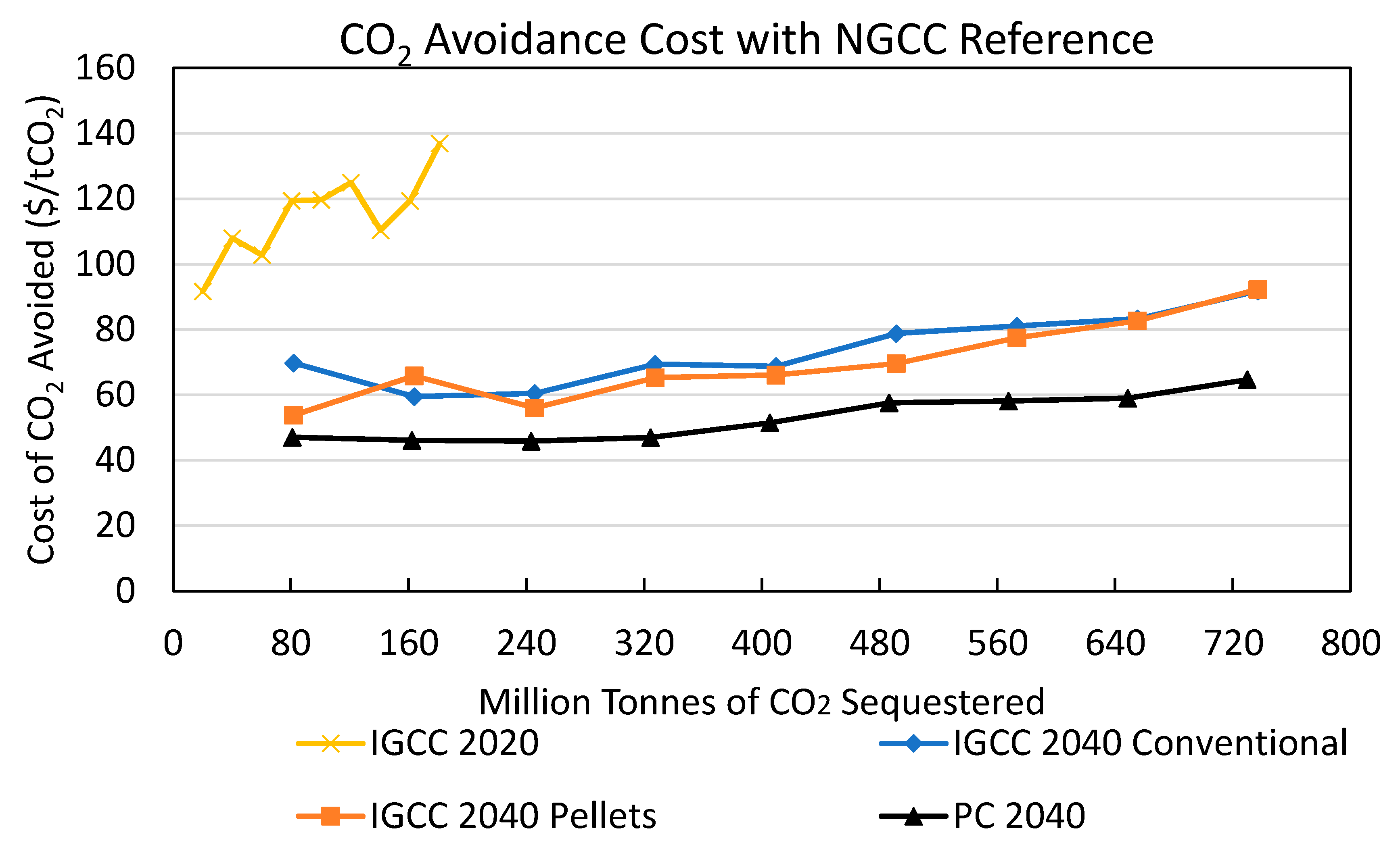
4. Discussion

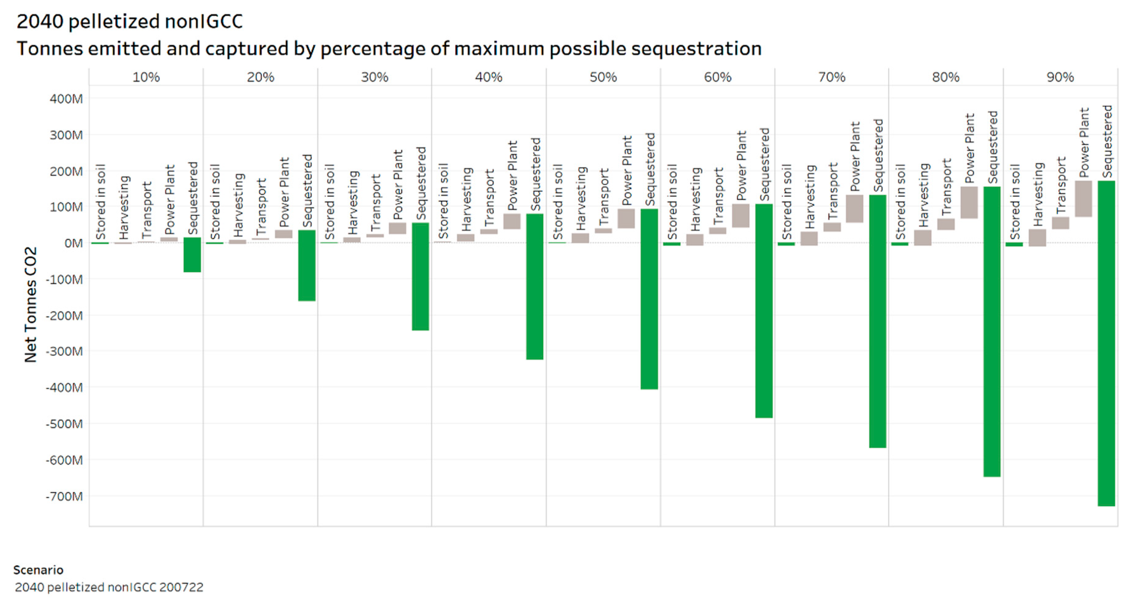
The maximum 90% CO₂ sequestration scenarios in Figure 9 and Figure 10 show capture of up 181 million tonnes CO₂ per year in 2020 and up to 737 million tonnes CO₂ per year in 2040. These results are within the range of CO₂ sequestration potential in the US that is constrained for colocation, storage, and injectivity (100–110 million tonnes CO₂ and 360–630 million tonnes CO₂ in 2020 and 2040, respectively) and the total potential (370–400 million tonnes CO₂ and 1040–1780 million tonnes CO₂ in 2020 and 2040, respectively) reported by Baik, Sanchez, Turner, Mach, Field, and Benson [8]. Differences are to be expected, as Baik et al. constrain biomass resources to those within (i.e., over) sequestration basins, whereas the present analysis allows for use of biomass resources from outside sequestration basins to the extent that CO₂ emissions from transporting biomass do not exceed sequestration benefits, and associated transportation costs are incurred. Costs shown above expressed as CAC range from $42 to $137 per tonne CO₂, which are within or below the $100 to $200 per tonne CO₂ reported by the IPCC ([4], Figure 4.2).

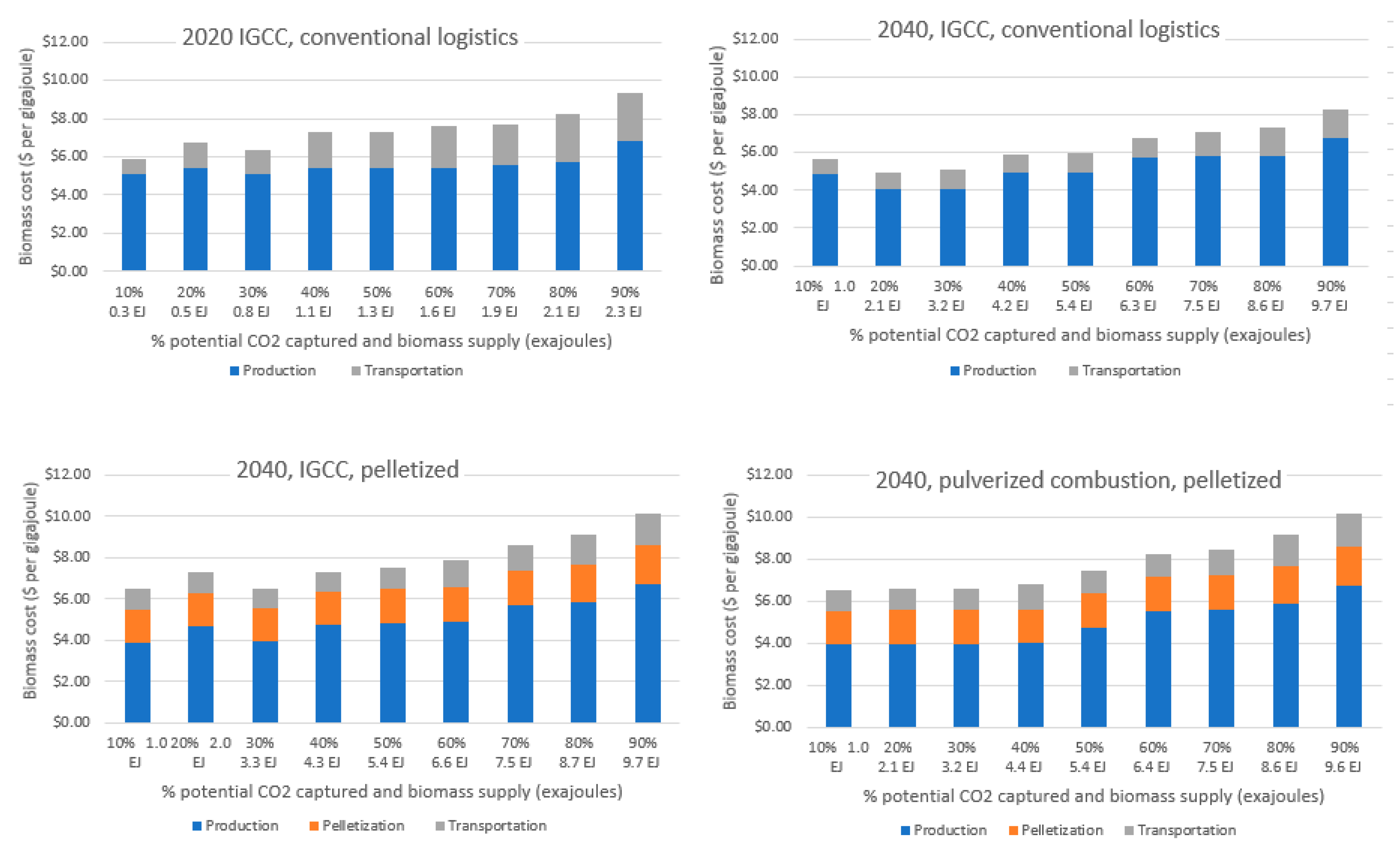
The results illustrate cost trends. Firstly, feedstock pelletization in the IGCC 2040 scenario results in a CAC about 6% cheaper. This is due to cost savings in transportation of the feedstock and higher energy density of the fuel because of lower moisture content of the feedstock. Secondly, as we increase the percentage of maximum CO₂ that can be sequestered through BECCS, the CAC increases. This makes sense because increasing demand for biomass requires the use of increasingly expensive and/or distant feedstock. However, the CACs reported in Figure 9 and Figure 10 are not all monotonically increasing as might be expected for supply curves, particularly for the IGCC 2020 conventional logistics scenario. These decreasing costs can be explained by increases in the energy intensity of the feedstock. In the long-term cases, the energy intensity of the feedstock (in MJ per dollar) is seen to decrease. This can be explained by the increase in the cost of fuel and the associated decrease in energy intensity of fuel with increasing demand for BECCS. The energy intensity of the fuel blend decreases once the higher energy-dense fuels, e.g., pine and switchgrass, have been consumed. In the IGCC 2020 case, however, due to the variance in feedstock availability in the near term, the energy intensity of the fuel initially increases sharply with increasing CO₂ sequestration levels, thus decreasing the cost of BECCS. Future work could account for this anomaly in the optimization.

The scenarios illustrated by the IPCC as alternative pathways to meet the Paris Agreement target estimate a requirement of 151, 414, and 1191 cumulative billion tonnes of CO₂ sequestration by BECCS by 2100 in Pathways 2, 3, and 4, respectively ([5], Figure SPM.3b). 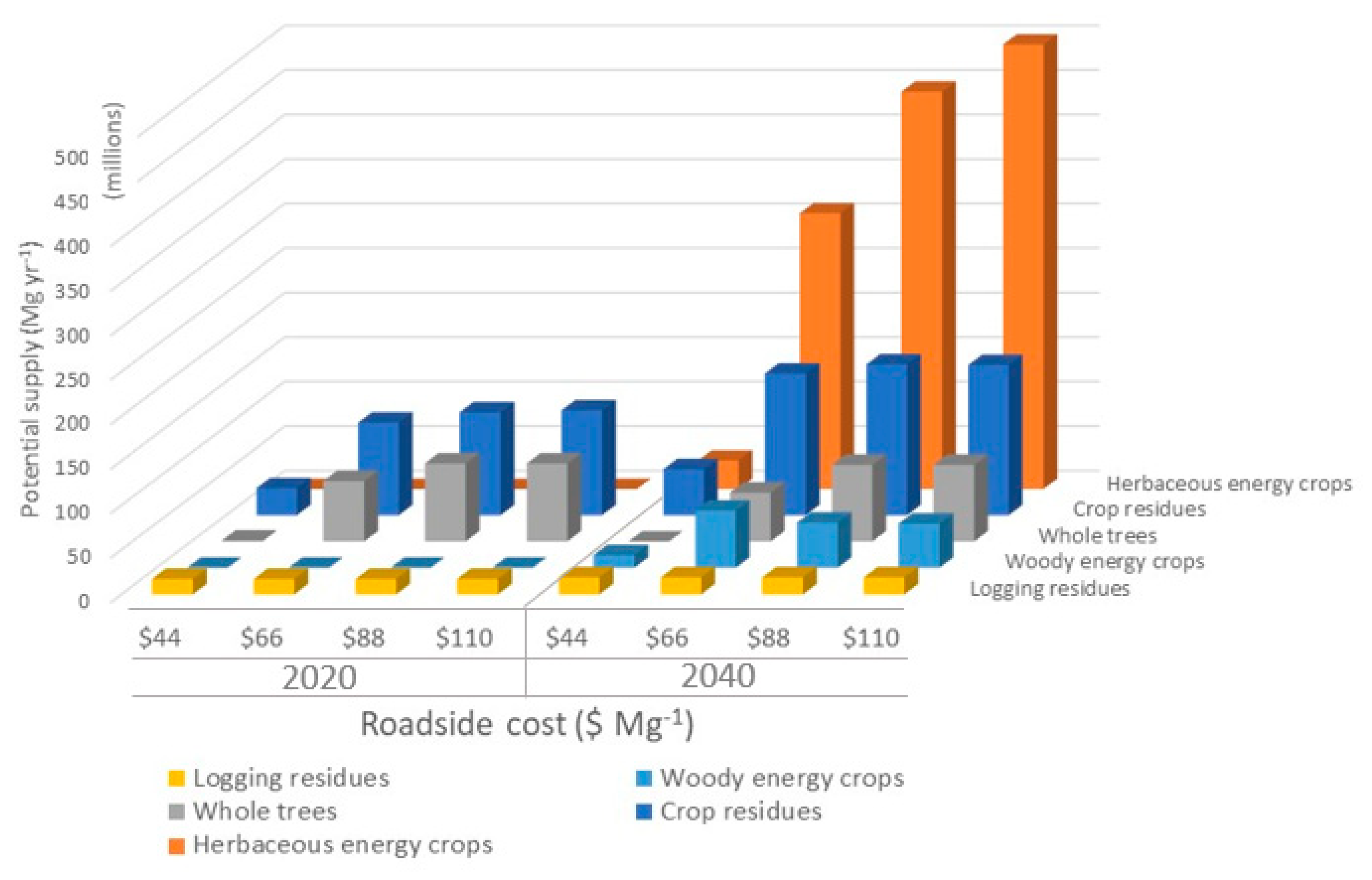To compare results presented in the present analysis with these IPCC estimates, assuming the total technical potential of 181 million tonnes CO₂ per year sequestered by BECCS in the US from 2030 to 2040, and 730 million tonnes CO₂ per year sequestered by BECCS from 2040 to 2100, this results in a cumulative estimated total technical potential of 46 billion tonnes CO₂ sequestered by BECCS in the US by 2100. This is equivalent to about 30%, 11%, and 4% of the targeted sequestration by BECCS by 2100 in Pathways 2, 3, and 4, respectively, in the IPCC. It is unknown how much of this total technical potential may be available. For example, competing demand for bioproducts could reduce the supply (or increase the price) of biomass available for BECCS. Alternatively, increased demand for bioenergy could provide opportunities for BECCS without competing for biomass resources. Of the results shown in Figure 9 and Figure 10, the 181 million tonnes CO₂ per year simulated in the near-term scenario used 206 million tonnes of the estimated 223 million tonnes of biomass reported available in 2020; the 730–811 million tonnes CO₂ sequestered in the future scenarios used 731–738 of the 823 million tonnes of biomass reported available in 2040 (Table 1, Figure 2, Tables S2 and S3).

It should also be taken into consideration that while costs shown here as CAC account for avoided emissions from reference scenarios as described in Equation (1), the calculations for the quantity of CO₂ sequestered do not take into consideration avoided emissions from the reference scenario. That is, if power from BECCS reduces demand for generation from pulverized coal or NGCC generation, then the CO₂ reduction benefit from BECCS would increase.

As discussed in the Introduction and Methods, it has been argued that some bioenergy systems in the absence of CCS may cause carbon emissions because of changes in the amount of biomass on the landscape [42,43], which may require some carbon-debt repayment period [44] before bioenergy can be considered carbon neutral as compared to a business-as-usual scenario. However, in the case of BECCS, 90% of the CO₂ produced from power generation is not emitted, but rather is sequestered below ground. This is unlike the case of bioenergy without CCS, in which case CO₂ produced from biomass is re-emitted to the atmosphere. Thus, with BECCs, because most of the carbon in harvested biomass is not emitted to the atmosphere, the carbon payback time (i.e., the time until plant growth and avoided fossil fuel emissions balance the CO₂ emitted, including supply chain emissions) will be much reduced compared with bioenergy without CCS. All woody resources used in this analysis have short payback periods, i.e., 4 years for willow, 8 years for poplars, and approximately 10–14 years for whole trees (<28 cm diameter at breast height). Of these, only the whole trees from forestlands, comprising 2–39% and 0–9% in the 2020 and 2040 scenarios, respectively, could have some carbon payback period depending on site-specific conditions. Site-specific carbon accounting would depend on previous land use, the expected business-as-usual scenario, and stand-specific silvicultural conditions, and is out of the scope of this analysis. In all scenarios, more than 80% of CO₂ from biomass used for BECCS is sequestered net of emissions from power generation, CCS, transportation, harvest, and production (Figure 13). Thus, in instances of whole trees from forestlands where a carbon debt repayment period may be applicable, any carbon debt repayment period would be reduced by more than 80%. Resources that incur a carbon payback period could be avoided, and feedstocks that provide carbon sequestration and other environmental services on the landscape could be incentivized.

5. Conclusions

BECCS and other NETs can reduce atmospheric CO₂. This analysis explores the potential supply and cost of BECCS under a range of feedstock, logistics, and power generation scenarios. Results of this study suggest using BECCS in the US has a total technical potential to sequester about 181 to 737 million tonnes of CO₂ annually in the near term and in 2040, respectively. In round estimates of cumulative potential, the US has a technical potential to sequester up to 46 billion tonnes CO₂ by BECCS by 2100. This is equivalent to about 30%, 11%, and 4% of the global sequestration by BECCS by 2100 in Pathways 2, 3, and 4, respectively, in the IPCC [5]. This US potential can be greatly reduced by future competing demands for biomass resources (e.g., cellulosic biofuels without BECCS) or potentially enabled by synergistic uses (e.g., demand for renewable power using BECCS). Scenario-specific average prices range from $42 to $137 per tonne CO₂ depending on cost accounting, power generation system, and biomass logistics system. Interactive visualization of results and output details are available at https://doi.org/10.11578/1647453.

These results use up to 92% of potential cellulosic biomass resources above current uses (after accounting for constraints for soil organic carbon, erosion, and competing conventional demands for food, feed, fiber, and exports), and thus represent an upper level of CO₂ sequestration potential. However, this study is not exhaustive of scenarios or opportunities to increase biomass supplies in the US. For example, cellulosic biomass energy crops used in this analysis are from the base case reported by USDOE (2016), resulting in about 370 million tonnes biomass per year, though future energy crop production increases to almost 670 million tonnes per year under the high-yield scenario (USDOE 2016), which is not used in this analysis. Over 100 million tonnes per year of waste resources and over 10 million tonnes per year of woody biomass from federally owned timberlands [6] were also excluded from this analysis and could be explored further. Results from USDOE (2016) do not necessarily represent the spatial distribution of demand for biomass that might respond to demand for BECCS, meaning biomass production could be better tailored to support BECCS in the future than the supplies used in this study. Resources in this analysis were limited to those deemed to have the potential to provide a range of positive environmental effects. If future scrutiny suggests that these environmental effects are in question, other resources such as wastes, hurricane and storm debris, thinnings in the wildland–urban interface to reduce fire risk, biomass from agroforestry systems, and removal of invasive exotic species, which are not included in this analysis, could be alternatively explored.

The authors would be remiss to not acknowledge questions raised in the literature (e.g., [41]) regarding the carbon neutrality of some bioenergy sources, particularly that woody biomass requires a regrowth or payback period before it is carbon neutral after being used for bioenergy. However, energy from resources that may have a significant carbon payback period if used without CCS would have a shortened payback period if used for BECCS, and would subsequently be net negative after the payback period. Of the biomass resources used for BECCS in this analysis, 2–39% and 0–9% in the 2020 and 2040 scenarios, respectively, are derived from small-diameter trees from forests that could have some carbon payback period depending on site-specific conditions if used for bioenergy without CCS. The large supply and diversity of potential biomass resources explored here provides the opportunity to focus BECCS on the fraction of resources that offer the most beneficial attributes based on locally and regionally determined sustainability criteria.

As an incipient concept, future research is needed to explore tradeoffs and opportunities related to BECCS in the US. As mentioned above, region- and site-specific conditions and practices can influence in situ carbon changes and should be explored on a case-by-case basis. Alternative biomass uses, e.g., biofuels, biochar, and other bioproducts, can compete with or provide synergies with BECCS. Given that feedstock quality specifications vary by application, approaches to feedstock fractionation can enable highest-value use of feedstock streams. Rail and barge transportation of biomass feedstocks was not included in this analysis but could provide low-emissions transportation and should be explored further. This analysis explored transporting biomass to sequestration basins, but an alternative approach is to transport CO₂ from power generation sites to sequestration basins, which could provide economic and logistical advantages and should also be explored. “Liability resources” such as biomass from storm and hurricane debris, wastes, and operations to control pine beetle infestations or invasive species were not included in this analysis and should be explored for maximum-benefit BECCS applications. Not included in this analysis is potential power demand as influenced by regional population expansion or climate change. For example, it may be anticipated that population growth in the US South coupled with climate change could increase demand for power in this region, which contains an abundance of biomass resources as well as potential sequestration basins with potential for BECCS. Potential cost-reduction strategies such as torrefaction, co-firing with coal, and implementation of existing biopower and infrastructure should also be explored.

6. Disclaimer and Acknowledgements

The views and opinions of the authors expressed herein do not necessarily state or reflect those of the United States Government or any agency thereof. Neither the United States Government nor any agency thereof, nor any of their employees, makes any warranty, expressed or implied, or assumes any legal liability or responsibility for the accuracy, completeness, or usefulness of any information, apparatus, product, or process disclosed, or represents that its use would not infringe privately owned rights.

This manuscript has been authored by UT-Battelle, LLC, under contract DE-AC05-00OR22725 with the US Department of Energy (DOE). The US government retains and the publisher, by accepting the article for publication, acknowledges that the US government retains a nonexclusive, paid-up, irrevocable, worldwide license to publish or reproduce the published form of this manuscript, or allow others to do so, for US government purposes. DOE will provide public access to these results of federally sponsored research in accordance with the DOE Public Access Plan (http://energy.gov/downloads/doe-public-access-plan).