Forecasting Seasonal Habitat Connectivity in a Developing Landscape

Abstract

Connectivity and wildlife corridors are often key components to successful conservation and management plans. Connectivity for wildlife is typically modeled in a static environment that reflects a single snapshot in time. However, it has been shown that, when compared with dynamic connectivity models, static models can underestimate connectivity and mask important population processes. Therefore, including dynamism in connectivity models is important if the goal is to predict functional connectivity. We incorporated four levels of dynamism (individual, daily, seasonal, and interannual) into an individual-based movement model for black bears (Ursus americanus) in Massachusetts, USA. We used future development projections to model movement into the year 2050. We summarized habitat connectivity over the 32-year simulation period as the number of simulated movement paths crossing each pixel in our study area. Our results predict black bears will further colonize the expanding part of their range in the state and move beyond this range towards the greater Boston metropolitan area. This information is useful to managers for predicting and addressing human–wildlife conflict and in targeting public education campaigns on bear awareness. Including dynamism in connectivity models can produce more realistic models and, when future projections are incorporated, can ensure the identification of areas that offer long-term functional connectivity for wildlife.

1. Introduction

In a developing world, providing connectivity for wildlife is widely recognized as an important component of successful conservation and management plans [1,2]. Connectivity allows wildlife to access resource patches during day-to-day movements, facilitates dispersal, encourages gene flow, and allows for range shifts and range expansion [2,3]. Connectivity, the implementation of which ranges from a single road crossing structure to large landscape corridors, is being included as a key part of many conservation plans [4], but well-connected protected areas are still relatively rare and globally fall well short of the Aichi Target 11 of the Convention on Biological Diversity [5]. More connectivity plans are therefore encouraged—and one of the components of successful connectivity plan implementation is the inclusion of one or more focal wildlife species [4].

Connectivity for wildlife is typically modeled in static environments and estimated for a single snapshot in time (e.g., [6,7]). However, wildlife responses to landscapes are inherently dynamic, as are the landscapes themselves (e.g., [8]). Dynamism can also exist among individuals. For example, individuals from the same population may have differing responses to the same landscape features [9,10], driven by differences among males and females, age classes, spatial locations, or temperament (e.g., boldness) [10,11,12]. There may also be differing behaviors and responses to landscape features throughout a diel period and across seasons [11,13]. In addition, interannual variability may exist due to disturbance-succession processes, climatic variation, human development, and other landscape changes [14]. All these types of dynamics may interact to affect functional habitat connectivity for a species.

Incorporating dynamism into wildlife connectivity models is important for several reasons. First, it allows for more realistic modeling and accurate estimates of connectivity. Dynamic connectivity models can increase our understanding of temporal changes in connectivity and population processes across space and time [15,16]. Simulation studies have found that static connectivity models can underestimate connectivity by an average of 30% compared with models that include space and time [16], and that dispersal-limited species may have a lower extinction threshold when modeled with dynamic landscapes compared to static ones [17]. Empirical studies have found that the importance of connectivity for wildlife population dynamics may be masked or misunderstood in static landscapes and therefore underestimated as a conservation need [15,18,19]. Furthermore, corridors derived from static connectivity models may differ substantially from those derived from dynamic models, resulting in a reduction of functional connectivity and a potential misallocation of conservation resources.

Dynamic connectivity can be modeled using different connectivity algorithms such as least-cost paths [20,21], resistant kernels [22], circuit theory [23,24], and, increasingly, individual-based movement models (IBMMs; e.g., [25,26]). In cost-path, kernel, and circuit theory approaches, resistance surfaces are typically derived for different temporal periods and connectivity is analyzed separately for each (e.g., [13,27]). The use of IBMMs is attractive because they provide a more mechanistic representation of functional connectivity by simulating the sequential movements of individuals in response to context-specific environmental conditions [28,29]. This allows simulated individuals to respond to a dynamic environment within a single model, resulting in a single summary output. Simulating sequential movements of individuals may be important for understanding movement response to future environmental conditions [30]—especially spatiotemporal dynamics of distributional shifts (e.g., range expansion, reintroductions) where the leading edges of species’ distributions are conditional upon individual locations at a given point in time [26,31]. IBMMs can also be parameterized with empirical data allowing for realistic simulations of movement and behavior for a population of interest [32]. Furthermore, the emergence of higher order patterns (e.g., home range size) from individual-level behaviors allows simulated patterns to be compared against empirical estimates of those patterns as a form of model calibration [33,34]. Connectivity estimates from IBMMs can be obtained by calculating the number or density of individuals moving through every pixel on the landscape [25,26,35].

We incorporated individual, daily, seasonal, and interannual dynamics into an IBMM for black bears (Ursus americanus) in the Commonwealth of Massachusetts, USA, to predict statewide functional connectivity. The black bear range in the state is expanding toward the greater Boston metropolitan area (MassWildlife unpublished data: https://www.mass.gov/service-details/learn-about-black-bears) and our goal was to predict movement routes and colonization in this expanding range. We simulated present-day and future movement on an annual basis from the current time step to the year 2050 and incorporated projected changes in human development into our models. We summarized density of movement from the IBMMs and identified areas where movement is likely to be concentrated in the future. Because black bears in Massachusetts are expanding their range towards more populated areas of the state, this information will be useful to managers for predicting and responding to human–wildlife conflict, as well as for targeting education campaigns.

2. Data and Methods

All analyses were conducted in R software [36].

2.1. Black Bear Data

Empirical data for parameterizing the IBMMs were from GPS-collared female black bears in central and western Massachusetts. Black bears were fitted with Telonics Gen 3 or Gen 4 collars programmed to acquire a fix every 45 min. Collar data was collected from 34 individuals between 2012 and 2017, totaling 65 bear-years (collar duration, number of fixes, and other collar information are provided in Appendix A). The GPS data were assessed for positional accuracy and fixes from the Gen 3 collar were removed if the position dilution of precision (PDOP) was > 5. Fixes from the Gen 4 collars were removed if the fix was unresolved, if the fix had a PDOP > 5 and was uncertain or was a 2D fix, or if the fix had a PDOP > 20 and was a certain or 3D fix. This filtering was performed to minimize the locational error to < 100 m and resulted in a mean data loss of 3.93% [37,38]. More capture, handling, and data processing procedures are detailed in Zeller et al. [11].

2.2. Resistance Surfaces

The IBMMs were modeled across resistance surfaces representing the ease or difficulty of bear movement across each grid cell in the study area. Individual black bears have varying movement responses to landscape features during different seasons and different times of day, which may translate into different resistance surfaces for each season/diel period [11]. Bears in our study area hibernate in the winter, and during the nonhibernation period they move the least in the spring and the most in the summer [11]. Movement response to different land cover types also changes seasonally [11]. During a 24-h period, bears tend to move more during the day than at night. However, daily movement patterns in our study area may change with season and for different land cover types [11]. To incorporate these movement dynamics into the IBMMs, we used six previously developed resistance surfaces reflecting bear movement: (1) spring/day, (2) spring/night, (3) summer/day, (4) summer/night, (5) fall/day, and (6) fall/night (Appendix B).

The resistance surface for each season/diel period was derived through the following four-step procedure (full details in Zeller et al. [11]). First, a step selection function was developed for each individual bear using only data for that season/diel period. Second, the step selection function was used to project the probability of movement across the study area. Third, the movement probability surfaces were combined across bears in a spatially-weighted approach following Osipova et al. [10] so that spatial differences in bear behavior and movement were maintained across the study area. Specifically, we created a Euclidean distance surface for each bear during each season/diel period from the centroid of that bear’s season/diel minimum convex polygon home range. We then took the inverse distance values and normalized them to sum to 1 across each surface and used the resulting surface to weight the individual movement probabilities at each grid cell. We summed the weighted movement probability surfaces to create a combined movement probability surface. Fourth, we created a resistance surface by calculating the linear inverse of the combined movement probability surface. These resistance surfaces have low resistances in grid cells with a high probability of movement and high resistances in grid cells with a low probability of movement. Resistance surfaces were rescaled from 0–1 to 1–10 for use in the IBMMs.

2.3. Step Length Distributions

The movement kernels for our IBMMs were based on empirical step length distributions from the collared bears. Bears in our study area move most in the summer and during daytime periods compared with other seasons and nighttime periods [11]. To reflect these differences, we calculated movement distributions for the same six seasons/diel periods as the resistance surfaces. Black bear step lengths followed a Pareto distribution and the shape and scale parameter of the Pareto distribution were estimated for each season/diel period with the gpd.fit function of the gPdtest package ([39]; Appendix D; Figure A2).

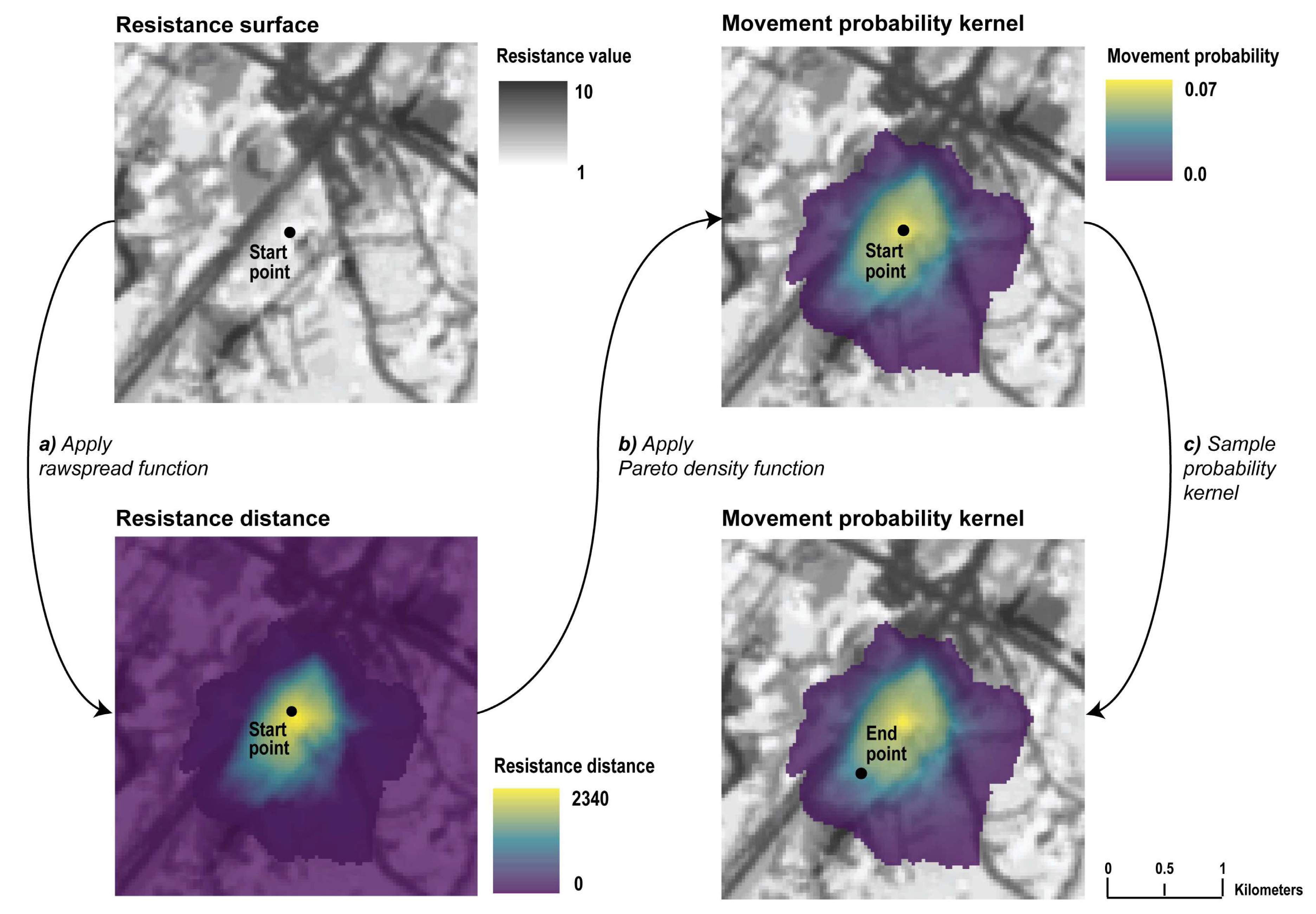
2.4. Individual-based Movement Model

The Massachusetts Division of Fisheries and Wildlife estimates there are approximately 5000 black bears in the western and central parts of the state (unpublished data). The highest density of bears is to the west of the Connecticut River, with densities diminishing to the east. An ‘expanding’ range has also been identified, which has a low number of recently established bears (Figure 1). To reflect these density changes, and the fact that we are only modeling female bears, we distributed 2000 simulated individuals to the west of the Connecticut River, 990 in the established range to the east of the Connecticut River, and 10 in the expanding range. Start points of these 3000 individuals were sampled probabilistically on the spring/day probability of movement surface (Figure 1). We assume that, by simulating females from home range data, our results will be conservative in terms of movement propagation. However, the focus on female movement is important at the expanding edge of ranges since they determine population establishment and whether reproduction is occurring in these areas.

We used a resistance kernel-based approach [22] to simulate individual bear movements that combined our empirical distributions of step lengths with our dynamic resistance surfaces to estimate the probability of an individual moving to any given pixel based on the intervening resistance values. At the beginning of each time step we first built a resistance kernel at the start point of each individual. We determined the individual’s maximum movement potential (i.e., the extent of the kernel) during a single time step in resistance distance units defined as the 97.5th quantile of the Pareto distribution derived from the parameters of the appropriate season/diel period. We hereafter refer to this quantity as an individual’s ‘bank account.’ We then calculated the resistance distance of every grid cell in the study area from the start point using the rawspread function in the gridprocess package [40] (Figure 2a). The extent of the resistance kernel stops when the bank account reaches a value of 0. In areas of low resistance, the bank account will be spent more slowly allowing the kernel to spread farther than in areas of high resistance. The output from the rawspread function provides a surface of proximity values to the start point. Therefore, we subtracted the values from one to obtain a resistance distance kernel.

We converted these resistance distance values to relative probability values using the Pareto distribution parameters of the appropriate season/diel period. This produced our final movement probability kernel (Figure 2b). The destination point (end point) for that time step was sampled from the movement probability kernel with the strata function of the sampling package (Figure 2c; [41]). This point then became the new start point and the procedure was repeated. We simulated steps for each bear at 45-min intervals from April 1 to November 15, the average den emergence and entry dates for our sample of bears, for a total of 7296 steps per individual. We started simulations on the spring/day resistance surface. We then alternated between the night resistance surface and Pareto parameters and the day resistance surface and Pareto parameters every 16 time-steps. We replaced the resistance surface and Pareto parameters from the spring with those of the summer at the 2369th time step and those of the summer with those of the fall at the 4172th time step. These changes corresponded with ecologically identified seasons for our collared population of black bears and with the dates of the GPS data used to estimate the seasonal resistance surfaces (see [11]).

We also describe the IBMM procedure with the standardized Overview, Design Concepts, and Details (ODD) protocol recommended by Grimm et al. [42,43] in Appendix D.

2.5. Model Validation and Calibration

We calculated the step lengths and minimum convex polygon home range sizes of our simulated individuals and compared them with our empirical sample of bears (described above) to determine how well our IBMMs represented movement and space use of black bears in our study area. Our first simulations resulted in comparatively short step lengths and small home range sizes (Appendix E). This is expected because the probability distribution (i.e., our Pareto distributions) used with a resistance kernel represents the maximum movement potential of an individual in a theoretical landscape with resistance = 1. In contrast, the observed step lengths used to estimate our Pareto distribution parameters occurred within real heterogeneous landscapes with varying resistances. Parameterizing a resistance kernel with an observed distribution of step lengths will therefore underestimate an individual’s movement potential and the extent of the movement probability kernel when applied to real resistant landscapes. Because we were unable to estimate the distribution of black bear step lengths in a nonresistant landscape, we increased the scale parameter of the Pareto distributions by 10% to allow our resistance kernels to more closely approximate a black bear’s maximum daily movement potential. This resulted in more realistic step lengths and home range sizes. Increasing the scale parameter above 10% resulted in unrealistically large home range sizes (Appendix E).

2.6. Future Projections

We used data from the Designing Sustainable Landscapes project (DSL, [44]) to incorporate future landscape change and predict bear movement on the expanding edge of their range in Massachusetts. The DSL urban growth model simulated human development across the northeastern US at 10-year time steps from 2020 to 2080 [45]. Resultant development categories were low-, medium-, and high-density development. We used the years 2020–2050 for our analysis. In the current time step, low-, medium-, and high-density development measured 5.5%, 3.7%, and 1.4% of the study area. In 2050, these development categories increased to 6.8%, 4.7%, and 2.5%, a percent increase of 24%, 27%, and 79% respectively. Over this time period, the human population in the state is projected to grow by at least 6% [46].

Most of our individual bear step selection function (SSF) models had development variables that matched the DSL categories. In those individuals, we used the DSL output directly in our future projections. However, approximately 30% of bear SSF models identified percent impervious surface as the most influential development variable. Therefore, we also transformed the DSL projections into percent impervious surfaces by reclassifying the low-, medium-, high-density development to 25%, 50%, and 100% impervious surface respectively. We combined these new percent impervious surfaces with our current (2019) percent impervious surface layer for each of the four future projection time steps. We predicted the SSF models for each bear for each season/diel period with these future projections, combined the projected probability of movement surfaces, and transformed them into resistance surfaces as described above.

We considered our first year of simulation to be 2019 and we simulated bear movement annually from 2019–2050. We used the last point from each simulated individual from the previous year as the start point for simulations in the next year. The 2020 resistance surfaces were used for the years 2020–2029, the 2030 resistance surfaces for 2030–2039 and so on. We summed the number of individual simulated paths crossing a pixel for each year and across all years to develop a movement density surface. Paths were derived by connecting all consecutive simulated points for each individual in each year.

3. Results

Our simulated individuals had a mean step length of 82.53 m (range: 0–2249 m) and a mean home range size of 77.97 km² (range: 6.85–228.44 km²). Our empirical bears had a mean step length of 193.34 m (range: 0–1998 m) and a mean home range size of 62.51 km² (range: 5.47–260.55 km²). Therefore, step lengths in our simulated bears are shorter, but home ranges are slightly larger than the empirical data. However, we did not include memory, territoriality, or interactions with conspecifics in our IBMMs and would therefore expect slightly shorter step lengths and larger home range sizes. Movement patterns and space use were visually similar among our simulated and empirical bears (e.g., Figure 3).

Projected human development from 2020 to 2050 resulted in fewer areas of low resistance and more areas of high resistance for bears. Across seasons and diel periods, the area covered by pixels with the lowest resistance values (1–2) decreased by an average of 32%, while the area covered by pixels with the highest resistance values (9–10) increased by an average of 159%.

Black bear space use in Massachusetts expanded eastward over the 32 years of simulations (Figure 4). Our results indicate that bear use may increase substantially in two relatively large areas in the expanding part of bear range (Figure 4e, large yellow circles). The first is from I-190 in the west to the Assabet River National Wildlife Refuge in the east and from State Route 2 in north to I-290 in the south. The second is from I-84 in the west to State Route 146 in the east, and I-90 to the north to the Connecticut and Rhode Island borders in the south. Two smaller areas also may see an increase in black bear use, the area just to the west of I-95 and the Cambridge Reservoir, and the area around the town of Carlisle, Massachusetts (Figure 4e, small yellow circles).

4. Discussion

We used an IBMM to model dynamic habitat connectivity for female black bears in Massachusetts, USA and found that black bears have high future movement potential within and beyond their expanding range in the state. We were able to incorporate individual, daily, seasonal, and interannual dynamics into our IBMM. Individual black bear differences were captured in the resistance surfaces used in the IBMMs by using the spatially-weighted approach presented by Osipova et al. [10]. This approach allows responses to landscape features to change depending on location. For example, bears in more developed areas of the state show lower avoidance of human development than more rural bears [11] and these differences are captured in these weighted surfaces. We also used resistance surfaces and movement parameters for two times of day and three seasons to capture movement and behavioral differences during these different periods. Lastly, we incorporated interannual dynamics by modeling IBMMs annually and incorporating future human development projections at 10-year time steps. By combining these four levels of dynamism, we were able to create realistic movement models and predict future connectivity.

IBMMs are well suited for modeling dynamic connectivity. As we demonstrated, they allow individuals to respond to changeable landscape features at different time steps and can integrate daily, seasonal, and interannual changes within a single model. More fundamentally, IBMMs allow population-level responses to emerge from the decisions made by thousands of individuals in response to local environmental conditions. This provides a more mechanistic approach for estimating dynamic landscape patterns of resource use and movement and, ultimately, functional connectivity. [32,47]. IBMMs have been used in this way to model dispersal corridors for 55 generations of little owls (Athene noctua) in Germany and Switzerland [26], connectivity under different land management scenarios for bighorn sheep (Ovis canadensis) in British Columbia, Canada [48], and connectivity for coral reef larvae using daily ocean current velocity data and different dispersal capabilities [25].

Modeling connectivity in a static environment may mask the importance of connectivity for maintaining wildlife population dynamics and may result in identifying corridors that are only periodically functional [15,16,18]. Because of the vast resources needed to conserve some wildlife corridors, it is not only important to model these corridors in a way that reflects behavioral and landscape dynamics, but also to ensure the longevity of these corridors into the future. To this end, we included future development projections in our IBMM and summarized connectivity at our final time step. If connectivity is being modeled at each time step separately (as with cost path, resistant kernel, or circuit theory approaches; e.g., [10,13]), identifying areas of consistent connectivity regardless of development or climate change is key to prioritizing conservation for long-term persistence of wildlife movement (e.g., Jennings et al. this issue).

Our IBMM was built using empirically derived resistance surfaces and movement step lengths and simulated reasonably realistic patterns of black bear movement and space use. Nevertheless, we recognize several areas in which our model could be improved. Our empirical population was comprised of females and all observed movements were within-home-range movements. Including males, especially young dispersers, would have likely resulted in longer step lengths and more movement. Female bears do not typically disperse far from their natal ranges [49,50]. However, this philopatry may be density dependent and females may disperse further in recently established black bear range [51]. Given that we could only model female home range movement, our model is a conservative approximation of movement and connectivity for our study area. Incorporating male bears and data from dispersing individuals would increase our insights into bear movement for the entire Massachusetts black bear population. A more direct incorporation of individual differences could also have been included in the IBMM by calculating step lengths and Pareto parameters for each individual bear and then assigning these parameters to each simulated individual based on a random draw. Other improvements to our model include incorporating births, natural deaths, and hunting take as well as different behavioral states, territoriality, and motivation [52]. Incorporating these parameters may have resulted in step lengths and home range sizes that were further aligned with our empirical bears, especially if step lengths were modeled as a function of land cover type. A more accurate understanding of spatial variation in current black bear density across our study area, particularly in the expanding portion of their range, may also improve our understanding of future landscape use of black bears. However, given the computational demands of our IBMM, we were unable to incorporate these model additions and are confident that our results are a reasonable approximation of black bear movement and connectivity in Massachusetts.

5. Conclusions

Incorporating dynamism into wildlife connectivity models increases their complexity, but also their realism. Using GPS collar data on black bears as well as future projections of human development, we were able to include four levels of dynamism—individual, daily and seasonal, and interannual dynamics -- within a single connectivity model. The increasing availability of animal tracking data as well as historical and future geospatial time series data increases our ability to model dynamic connectivity for wildlife. Ensuring realism and future longevity of wildlife corridors will be important for the success of corridor conservation initiatives in providing long-term functional connectivity for wildlife. With our IBMM, we predicted black bears will increase their colonization within the current boundary of their expanding range in Massachusetts and will move beyond this boundary into uninhabited areas of the state. The model developed here might be combined with other information to determine the location, amount, and spatial configuration of public education needed to reduce human–bear conflicts (e.g., [53]), or where ordinances may be implemented to remove food attractants. The model may also be used to identify road-crossing hotspots that may be the target of mitigation measures. As black bears are expected to continue to move towards and colonize more populated areas around the greater Boston metropolitan area, information on where this movement and colonization may occur is important for developing effective management strategies for preventing human–wildlife conflict.

References

1. Rudnick, D.; Beier, P.; Cushman, S.; Dieffenbach, F.; Epps, C.W.; Gerber, L.; Hartter, J.; Jenness, J.; Kintsch, J.; Merenlender, A.M.; et al. The Role of Landscape Connectivity in Planning and Implementing Conservation and Restoration Priorities; Issues in Ecology. Report No. 16.; Ecological Society of America: Washington, DC, USA, 2012. [Google Scholar]
2. Hilty, J.A.; Keeley, A.T.H.; Lidicker, W.Z., Jr.; Merenlender, A.M. Corridor Ecology, 2nd ed.: Linking Landscapes for Biodiversity Conservation and Climate Adaptation; Island Press: Washington, DC, USA, 2019. [Google Scholar]
3. Chen, I.-C.; Hill, J.K.; Ohlemüller, R.; Roy, D.B.; Thomas, C.D. Rapid Range Shifts of Species Associated with High Levels of Climate Warming. Science 2011, 333, 1024–1026. [Google Scholar] [CrossRef] [PubMed]
4. Keeley, A.T.H.; Beier, P.; Creech, T.; Jones, K.; Jongman, R.H.; Stonecipher, G.; Tabor, G.M. Thirty years of connectivity conservation planning: An assessment of factors influencing plan implementation. Environ. Res. Lett. 2019, 14, 103001. [Google Scholar] [CrossRef]
5. Saura, S.; Bertzky, B.; Bastin, L.; Battistella, L.; Mandrici, A.; Dubois, G. Protected area connectivity: Shortfalls in global targets and country-level priorities. Biol. Conserv. 2018, 219, 53–67. [Google Scholar] [CrossRef] [PubMed]
6. Koen, E.L.; Bowman, J.; Sadowski, C.; Walpole, A.A. Landscape connectivity for wildlife: Development and validation of multispecies linkage maps. Methods Ecol. Evol. 2014, 5, 626–633. [Google Scholar] [CrossRef]
7. Proctor, M.F.; Nielsen, S.E.; Kasworm, W.F.; Servheen, C.; Radandt, T.G.; MacHutchon, A.G.; Boyce, M.S. Grizzly bear connectivity mapping in the Canada-United States trans-border region. J. Wildl. Manag. 2015, 79, 544–558. [Google Scholar] [CrossRef]
8. Mueller, T.; Olson, K.A.; Fuller, T.K.; Schaller, G.B.; Murray, M.G.; Leimgruber, P. In search of forage: Predicting dynamic habitats of Mongolian gazelles using satellite-based estimates of vegetation productivity. J. Appl. Ecol. 2008, 45, 649–658. [Google Scholar] [CrossRef]
9. Bélisle, M. Measuring Landscape Connectivity: The Challenge of Behavioral Landscape Ecology. Ecology 2005, 86, 1988–1995. [Google Scholar] [CrossRef] [Green Version]
10. Osipova, L.; Okello, M.M.; Njumbi, S.J.; Ngene, S.; Western, D.; Hayward, M.; Balkenhol, N. Using step-selection functions to model landscape connectivity for African elephants: Accounting for variability across individuals and seasons. Anim. Conserv. 2018, 22, 35–48. [Google Scholar] [CrossRef]
11. Zeller, K.A.; Wattles, D.W.; Conlee, L.; DeStefano, S. Black bears alter movements in response to anthropogenic features with time of day and season. Mov. Ecol. 2019, 7, 19. [Google Scholar] [CrossRef]
12. Wolf, M.; Weissing, F.J. Animal personalities: Consequences for ecology and evolution. Trends Ecol. Evol. 2012, 27, 452–461. [Google Scholar] [CrossRef]
13. Chetkiewicz, C.-L.B.; Boyce, M.S. Use of resource selection functions to identify conservation corridors. J. Appl. Ecol. 2009, 46, 1036–1047. [Google Scholar] [CrossRef]
14. Parks, S.A.; Carroll, C.; Dobrowski, S.Z.; Allred, B.W. Human land uses reduce climate connectivity across North America. Glob. Chang. Biol. 2020, 26, 2944–2955. [Google Scholar] [CrossRef] [PubMed]
15. Kool, J.; Moilanen, A.; Treml, E.A. Population connectivity: Recent advances and new perspectives. Landsc. Ecol. 2012, 28, 165–185. [Google Scholar] [CrossRef]
16. Martensen, A.C.; Saura, S.; Fortin, M.-J. Spatio-temporal connectivity: Assessing the amount of reachable habitat in dynamic landscapes. Methods Ecol. Evol. 2017, 8, 1253–1264. [Google Scholar] [CrossRef]
17. Wimberly, M.C. Species Dynamics in Disturbed Landscapes: When does a Shifting Habitat Mosaic Enhance Connectivity? Landsc. Ecol. 2006, 21, 35–46. [Google Scholar] [CrossRef]
18. Hodgson, J.; Moilanen, A.; Thomas, C.D. Metapopulation responses to patch connectivity and quality are masked by successional habitat dynamics. Ecology 2009, 90, 1608–1619. [Google Scholar] [CrossRef] [Green Version]
19. Roe, J.H.; Brinton, A.C.; Georges, A. Temporal and spatial variation in landscape connectivity for a freshwater turtle in a temporally dynamic wetland system. Ecol. Appl. 2009, 19, 1288–1299. [Google Scholar] [CrossRef]
20. Adriaensen, F.; Chardon, J.; De Blust, G.; Swinnen, E.; Villalba, S.; Gulinck, H.; Matthysen, E. The application of ‘least-cost’ modelling as a functional landscape model. Landsc. Urban Plan. 2003, 64, 233–247. [Google Scholar] [CrossRef]
21. Loro, M.; Ortega, E.; Arce, R.M.; Geneletti, D. Ecological connectivity analysis to reduce the barrier effect of roads. An innovative graph-theory approach to define wildlife corridors with multiple paths and without bottlenecks. Landsc. Urban Plan. 2015, 139, 149–162. [Google Scholar] [CrossRef] [Green Version]
22. Compton, B.W.; McGarigal, K.; Cushman, S.A.; Gamble, L.R. A Resistant-Kernel Model of Connectivity for Amphibians that Breed in Vernal Pools. Conserv. Biol. 2007, 21, 788–799. [Google Scholar] [CrossRef]
23. McRae, B.H.; Dickson, B.; Keitt, T.H.; Shah, V.B. Using Circuit Theory to Model Connectivity in Ecology, Evolution, and Conservation. Ecology 2008, 89, 2712–2724. [Google Scholar] [CrossRef] [PubMed]
24. McRae, B.H.; Hall, S.A.; Beier, P.; Theobald, D.M. Where to Restore Ecological Connectivity? Detecting Barriers and Quantifying Restoration Benefits. PLoS ONE 2012, 7, e52604. [Google Scholar] [CrossRef]
25. Kool, J.; Paris, C.B.; Barber, P.H.; Cowen, R.K. Connectivity and the development of population genetic structure in Indo-West Pacific coral reef communities. Glob. Ecol. Biogeogr. 2011, 20, 695–706. [Google Scholar] [CrossRef]
26. Hauenstein, S.; Fattebert, J.; Grüebler, M.U.; Naef-Daenzer, B.; Pe’er, G.; Hartig, F. Calibrating an individual-based movement model to predict functional connectivity for little owls. Ecol. Appl. 2019, 29, e01873. [Google Scholar] [CrossRef] [PubMed]
27. Mui, A.; Caverhill, B.; Johnson, B.; Fortin, M.-J.; He, Y. Using multiple metrics to estimate seasonal landscape connectivity for Blanding’s turtles (Emydoidea blandingii) in a fragmented landscape. Landsc. Ecol. 2016, 32, 531–546. [Google Scholar] [CrossRef]
28. Grimm, V.; Railsback, S.F. Individual-based Modeling and Ecology; Princeton University Press: Princeton, NJ, USA, 2005. [Google Scholar]
29. McLane, A.J.; Semeniuk, C.; McDermid, G.J.; Marceau, D.J. The role of agent-based models in wildlife ecology and management. Ecol. Model. 2011, 222, 1544–1556. [Google Scholar] [CrossRef]
30. Wood, K.A.; Stillman, R.A.; Hilton, G.M. Conservation in a changing world needs predictive models. Anim. Conserv. 2017, 21, 87–88. [Google Scholar] [CrossRef] [Green Version]
31. Kramer-Schadt, S.; Revilla, E.; Wiegand, T. Lynx reintroductions in fragmented landscapes of Germany: Projects with a future or misunderstood wildlife conservation? Biol. Conserv. 2005, 125, 169–182. [Google Scholar] [CrossRef]
32. DeAngelis, D.L.; Grimm, V. Individual-based models in ecology after four decades. F1000Prime Rep. 2014, 6. [Google Scholar] [CrossRef] [Green Version]
33. Bauduin, S.; McIntire, E.; St-Laurent, M.-H.; Cumming, S. Overcoming challenges of sparse telemetry data to estimate caribou movement. Ecol. Model. 2016, 335, 24–34. [Google Scholar] [CrossRef]
34. Wiegand, T.; Jeltsch, F.; Hanski, I.; Grimm, V. Using pattern-oriented modeling for revealing hidden information: A key for reconciling ecological theory and application. Oikos 2003, 100, 209–222. [Google Scholar] [CrossRef] [Green Version]
35. Pe’Er, G.; Kramer-Schadt, S. Incorporating the perceptual range of animals into connectivity models. Ecol. Model. 2008, 213, 73–85. [Google Scholar] [CrossRef]
36. R Core Team. R: A language and Environment for Statistical Computing. Version 3.6.2. 2019. Available online: https://cran.r-project.org/ (accessed on 6 December 2019).
37. Lewis, J.S.; Rachlow, J.L.; Garton, E.O.; Vierling, L.A. Effects of habitat on GPS collar performance: Using data screening to reduce location error. J. Appl. Ecol. 2007, 44, 663–671. [Google Scholar] [CrossRef]
38. Telonics. Gen 4 GPS Systems Manual. Telonics, Inc., 2012. Available online: www.telonics.com. (accessed on 1 March 2018).
39. Estrada, E.G.; Alva, J.A.V. Gpdtest: Bootstrap Goodness-Of-Fit Test for the Generalized Pareto Distribution. Version 0.4. 2012. Available online: https://cran.r-project.org/web/packages/gPdtest/ (accessed on 26 April 2019).
40. Plunkett, E.B. Gridprocess: Package for Processing Raster Data. Version 0.1.3. 2019. Available online: https://github.com/ethanplunkett/gridprocess (accessed on 4 June 2019).
41. Tillé, Y.; Matei, A. Sampling: Survey Sampling. Version 2.8. 2016. Available online: https://CRAN.R-project.org/package=sampling (accessed on 22 September 2016).
42. Grimm, V.; Berger, U.; Bastiansen, F.; Eliassen, S.; Ginot, V.; Giske, J.; Goss-Custard, J.; Grand, T.; Heinz, S.K.; Huse, G.; et al. A standard protocol for describing individual-based and agent-based models. Ecol. Model. 2006, 198, 115–126. [Google Scholar] [CrossRef]
43. Grimm, V.; Berger, U.; DeAngelis, D.L.; Polhill, J.G.; Giske, J.; Railsback, S.F.; Polhill, N.M.G.J.G. The ODD protocol: A review and first update. Ecol. Model. 2010, 221, 2760–2768. [Google Scholar] [CrossRef] [Green Version]
44. McGarigal, K.; Compton, B.W.; Plunkett, E.B.; DeLuca, W.V.; Grand, J. Designing sustainable landscapes project. University of Massachusetts, Amherst. 2017. Available online: www.umass.edu/landeco/research/dsl/dsl.html (accessed on 10 March 2020).
45. McGarigal, K.; Plunkett, E.B.; Willey, L.L.; Compton, B.W.; DeLuca, W.; Grand, J. Modeling non-stationary urban growth: The SPRAWL model and the ecological impacts of development. Landsc. Urban Plan. 2018, 177, 178–190. [Google Scholar] [CrossRef]
46. UMass Donahue Institute. Population Projections. UMass Donahue Institute, MassDOT Vintage. 2018. Available online: pep.donahue-institute.org (accessed on 7 April 2020).
47. Pe’er, G.; Henle, K.; Dislich, C.; Frank, K. Breaking Functional Connectivity into Components: A Novel Approach Using an Individual-Based Model, and First Outcomes. PLoS ONE 2011, 6, e22355. [Google Scholar]
48. Allen, C.H.; Parrott, L.; Kyle, C. An individual-based modelling approach to estimate landscape connectivity for bighorn sheep (Ovis canadensis). PeerJ 2016, 4. [Google Scholar] [CrossRef] [Green Version]
49. Costello, C.M. Estimates of dispersal and home-range fidelity in American black bears. J. Mammal. 2010, 91, 116–121. [Google Scholar] [CrossRef]
50. Rogers, L.L. Effects of Food Supply and Kinship on Social Behavior, Movements, and Population Growth of Black Bears in Northeastern Minnesota. Wildl. Monogr. 1987, 97, 3–72. [Google Scholar]
51. Kristensen, T.V.; Puckett, E.E.; Landguth, E.L.; Belant, J.L.; Hast, J.T.; Carpenter, C.; Sajecki, J.L.; Beringer, J.; Means, M.; Cox, J.J.; et al. Spatial genetic structure in American black bears (Ursus americanus): Female philopatry is variable and related to population history. Heredity 2017, 120, 329–341. [Google Scholar] [CrossRef] [PubMed]
52. Avgar, T.; Deardon, R.; Fryxell, J.M. An empirically parameterized individual based model of animal movement, perception, and memory. Ecol. Model. 2013, 251, 158–172. [Google Scholar] [CrossRef]
53. Marley, J.; Hyde, A.; Salkeld, J.H.; Prima, M.-C.; Parrott, L.; Senger, S.E.; Tyson, R.C. Does human education reduce conflicts between humans and bears? An agent-based modelling approach. Ecol. Model. 2017, 343, 15–24. [Google Scholar] [CrossRef]
Figure 1. Black bear range in Massachusetts and distribution of start points for 3000 simulated individuals. In the western range, 2000 individuals were initiated, in the eastern range, 990, and in the expanding range, 10.
Land 09 00233 g001
Figure 2. Procedure for simulating one step for the black bear individual-based movement models (IBMMs). From a start point on the resistance surface, (a) we applied and took the inverse of the rawspread function [40] which calculates resistance distance from the start point. We then (b) applied the Pareto density function of the appropriate diel period and season to the resistance distance surface to create a movement probability kernel and transformed the kernel to sum to 1. We then (c) probabilistically sampled a destination (end) point on the movement probability kernel.
Land 09 00233 g002
Figure 3. Examples of empirical black bear paths (in black) and simulated black bear paths in the same area (in blue). The background map shows roads in white, water bodies in dark grey and conserved lands in green.
Land 09 00233 g003
Figure 4. Per-pixel sum of simulated black bear paths for (a) 2019, (b) 2030, (c) 2040, (d) 2050, and (e) all years (2019 to 2050). From west to east, the black polygons represent black bear range to the west of the Connecticut River, to the east of the river, and the expanding range. Yellow circles indicate areas with substantial future black bear use in their expanding range. The locations of the two larger and smaller circles are described further in the Results section.
Land 09 00233 g004