Article

Temporal Resource Continuity Increases Predator Abundance in a Metapopulation Model: Insights for Conservation and Biocontrol

1
Department of Entomology, Kansas State University, Manhattan, KS 66506, USA
2
Department of Integrative Biology, University of Wisconsin-Madison, Madison, WI 53726, USA
3
Department of Entomology, University of Wisconsin-Madison, Madison, WI 53726, USA
*
Author to whom correspondence should be addressed.
Land 2020, 9(12), 479; https://doi.org/10.3390/land9120479
Submission received: 18 October 2020 / Revised: 24 November 2020 / Accepted: 24 November 2020 / Published: 28 November 2020
(This article belongs to the Section Landscape Ecology)

Abstract

:
The amount of habitat in a landscape is an important metric for evaluating the effects of land cover on biodiversity, yet it fails to capture complex temporal dimensions of resource availability that could be consequential for species population dynamics. Here, we use a spatially-explicit predator–prey metapopulation model to test the effect of different spatiotemporal resource patterns on insect predators and their prey. We examined population responses in model landscapes that varied in both the amount and temporal variability of basal vegetation. Further, we examined cases where prey comprised either a single generalist species or two specialist species that use different resources available either early or late in the growing season. We found that predators and generalist prey benefitted from lower temporal variance of basal resources, which increased landscape-scale abundances. However, increasing the amount of basal resources also increased the variability of generalist prey populations. Specialist prey, on the other hand, did not benefit from less temporally variable basal resources, as they were restricted by habitat type, while also suffering greater predation. Predators achieved greater prey suppression in landscapes with less temporally variable resources, but the overall effects on prey abundance depended on prey habitat specialization. Our simulations demonstrate the joint importance of both the amount and temporal variability of resources for understanding how landscape heterogeneity influences biodiversity and ecosystem services such as the biological control of agricultural pests.

1. Introduction

The abundance and diversity of species in a landscape generally increase with greater habitat area [1], presumably because larger areas can provide more limiting resources to consumers. This is a central principle of biodiversity conservation and the conservation of beneficial species that provide ecosystem services in working landscapes. For example, increasing non-crop habitat surrounding agricultural fields can promote insect abundance, diversity, pollination, and natural pest control [2,3,4,5,6]. Yet, a facile understanding of habitat versus non-habitat or cropland versus natural area ignores the substantial heterogeneity that exists within land use categories [6] as well as the complex temporal dynamics of mobile consumers and their resources [7,8,9].
“Landscape complementation” describes the processes in which mobile organisms acquire key resources by traversing multiple patch types in a landscape [10]. This process may be especially important in agriculturally-dominated landscapes, where temporal gaps or bottlenecks in food availability brought about by landscape simplification—e.g., increasing annual cropland area or decreasing crop diversity—may negatively affect beneficial species that require nourishment continuously throughout the growing season [8]. Differences in the composition of habitats between landscapes can result in differential temporal patterns of resource availability for mobile consumers. In homogenous landscapes, temporal gaps could result if ephemeral resources emerge synchronously across different patches (Figure 1A,C) and then disappear for the rest of the growing season (e.g., before planting or after harvesting in a monocropped landscape). Although mobile organisms could travel within a landscape to access potential food resources in different locations, there may be temporal gaps at critical points in the organism’s life cycle that could affect growth, survival, and reproduction. On the other hand, food resources in different habitat patches could emerge asynchronously (Figure 1B,D). Such asynchrony creates an ensemble of temporally complementary patches that minimizes resource gaps and, for mobile species, results in continuous resource provisioning at a landscape scale over the course of a season (e.g., in a landscape of phenologically divergent annual and perennial crops). We refer to this process as “temporal resource complementation”.
The value of temporal resource complementation has received empirical support in beneficial insects such as wild bees, which can benefit from the existence of temporally asynchronous floral resources in heterogeneous landscapes [11,12,13]. However, less is known about how temporal resource complementation affects predatory arthropods, the dynamics of tritrophic interactions, and the consequences for conservation biological control [9]. A population of mobile predators may track ephemeral prey resources across a landscape as they emerge in one location, decline, and then emerge in another. Yet, a predator population’s ability to track herbivorous prey depends on the prey’s ability to track their own resources, constituted by the vegetation present in the landscape (hereafter, “basal resources”). Habitat-generalist prey may benefit more from temporal resource complementation than habitat-specialists if mobile generalists can utilize multiple basal resource types that emerge in different locations throughout the season. Such generalist prey may thus support larger predator populations over time than would specialist prey. However, it is not clear whether (1) an increase in predator population size would enhance generalist prey suppression or (2) lower predator density could maintain suppression of specialist prey. This latter scenario might be especially relevant to biological control in agroecosystems, where many pests specialize on particular crop types (e.g., cereals or legumes), but are frequently consumed by generalist predators such as spiders or lady beetles.
Because of the difficulty of conducting empirical studies rigorously investigating the spatio-temporal dynamics of insect populations across multiple generations, modeling approaches are frequently employed [14,15,16]. For example, Le Gal et al. [17] recently modeled the effect of overwintering (i.e., seminatural) habitat amount and arthropod species traits on multiple indicators of pest control services, finding that landscapes with more overwintering habitat supported earlier visitation and improved pest suppression by natural enemies; yet the study does not consider how temporal heterogeneity in the crop mosaic itself “cascades up” to higher trophic levels when predators are foraging. Here, we use a spatially-explicit predator–prey metapopulation model [18] to examine how patchy landscapes differing in the amount and continuity of basal resources affect the population dynamics of mobile arthropod herbivores (specialist or generalist prey) and, in turn, their arthropod natural enemies (generalist predators). Although specialist natural enemies (such as many parasitoids) are often important biological control agents, we do not include them in our analysis because they are intimately tied to their hosts and thus would be unaffected by our definition of temporal complementation (i.e., the use of prey resources in multiple habitat types with distinct phenologies). Model landscapes are comprised of patches where ephemeral resources emerge either early or late in a growing season. This allows us to simulate different amounts of basal resources within and across a growing season as well as different levels of resource continuity, which we measure as the landscape-scale temporal variance of basal resources across time (hereafter, “temporal variance”) (see Supplementary Materials).
In accordance with conventional wisdom, we expected that landscapes with a greater total amount of basal resources would support larger prey and predator populations. However, we predicted that greater temporal continuity (i.e., lower temporal variance and greater temporal complementation), independent of resource amount, would increase population sizes owing to less frequent landscape-scale temporal resource gaps [8]. We compare the response of a predator–prey system with a single generalist prey species that can use both early- and late-season resource patches to that of a system with two habitat specialists, each of which specializes on resources in different habitats that emerge either early or late in the growing season. We predicted that a system with one generalist prey species would support larger predator populations than a system with two specialist prey species under the same season-long resource conditions.

2. Materials and Methods

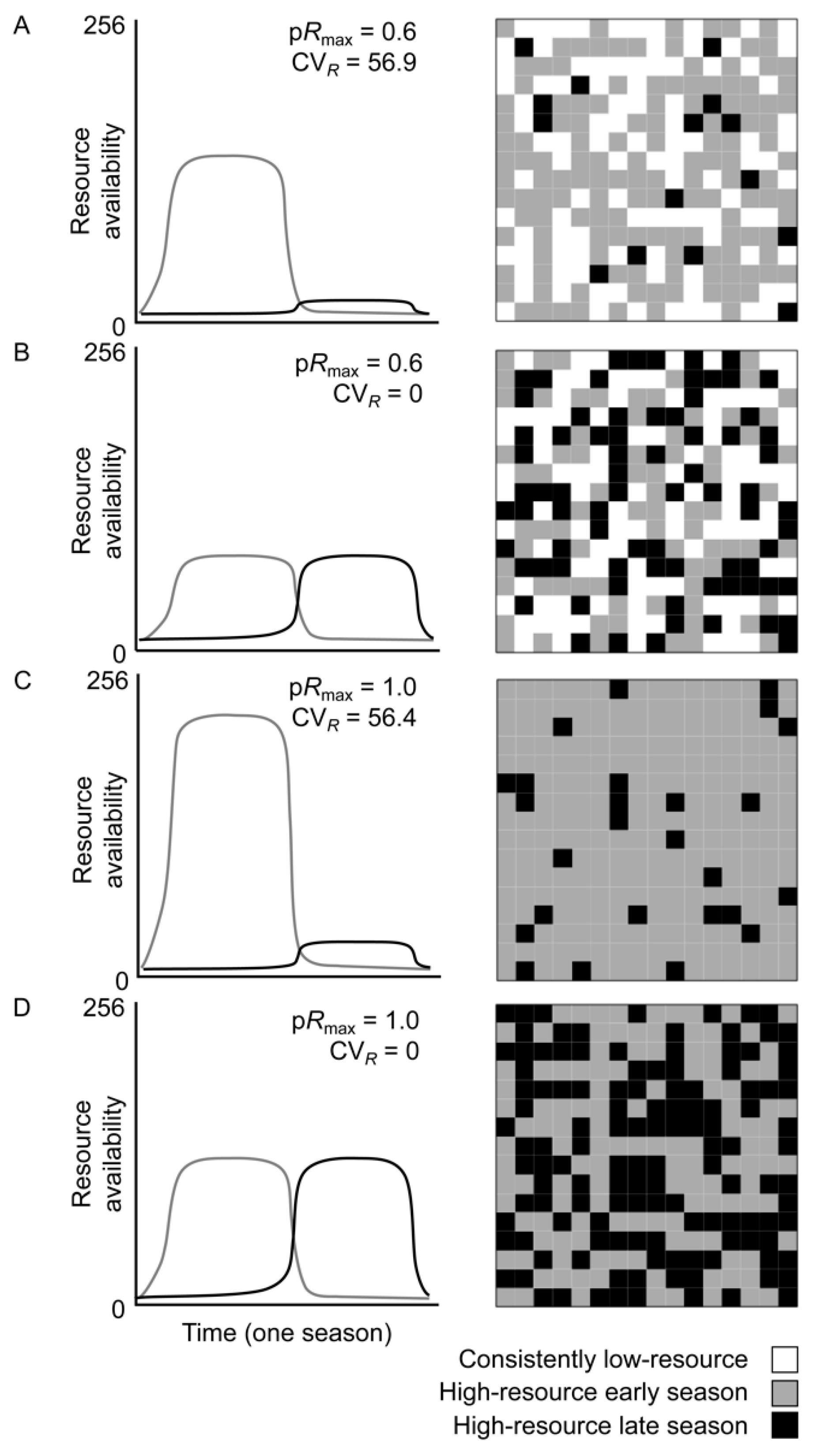
2.1. Model Landscapes

Predator and prey population dynamics were modeled in each cell of a 16 × 16-cell lattice, representing a square landscape with 256 patches (e.g., Figure 1). Patches vary in their capacity to provision basal resources, which determines the carrying capacity (K) of prey populations. The habitat in each patch x at location i can switch mid-season between a high-resource state (xi = 1), which offers relatively abundant basal food resources for prey populations, or a low-resource state (xi = 0), which offers relatively few resources for prey. We thus defined three patch types: (1) early-season high-resource (e.g., early-season crop); (2) late-season high-resource (e.g., late-season crop); or (3) continuously low-resource (e.g., highly disturbed or developed area). Because our focus in this study is investigating the potential role of cropland as habitat and simulating dynamics of predators and prey in managed agricultural landscapes, we intentionally exclude a fourth potential resource state, one of continuously high-resources (e.g., diverse natural habitats that have resources early and late in the season). By varying the number and location of high-resource patches in each half of the growing season, we can generate model landscapes with different combinations of basal resource amount and temporal variance (Figure 1). We quantify the total, or season-long, amount of basal resources R in a landscape as the sum of resource state values in the first and second half (A and B) of the growing season:
R = i = 1 256 ( x i A + x i B )
Thus, R can vary between 0 and 256 in our model landscapes. Landscape-scale temporal variance in basal resource amount is the variance in sum of patch values between the first and second half of the season:
σ R 2 = v a r ( i = 1 256 x i A , i = 1 256 x i B )
Because R varies among model landscapes, we use the coefficient of variation of (CVR) to standardize for the level of R, where
CV R = σ R 2 R
Thus, for a given level of R, high CVR values indicate landscapes where resources are synchronously available and concentrated in only half of the growing season, which creates a “gap”, or period of low resource availability, during the other half of the season (Figure 1A,C). In contrast, low CVR values indicate landscapes where resources are asynchronously available and more evenly distributed throughout the growing season (Figure 1B,D).

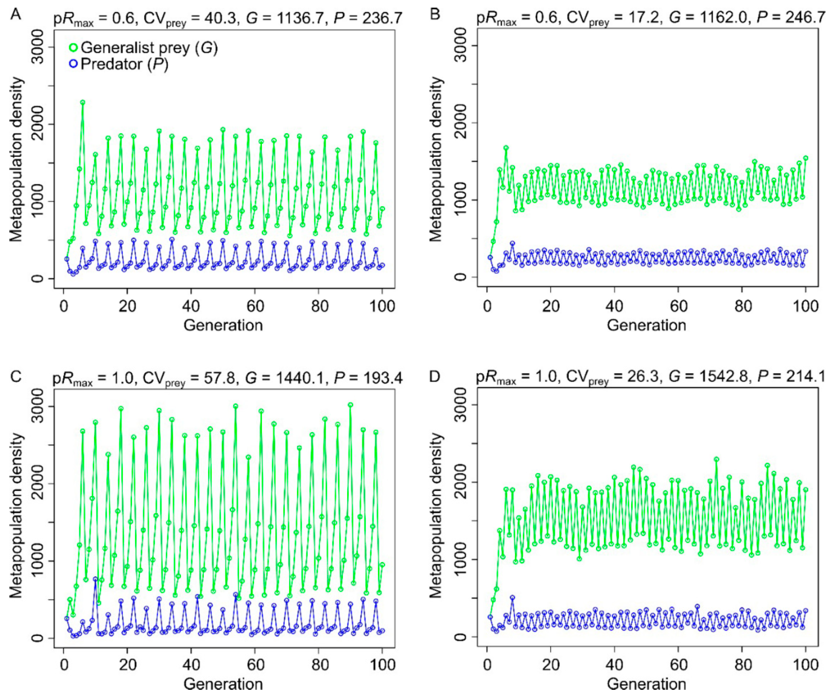
2.2. Predator–Prey Metapopulation Model

We modeled the spatially-explicit metapopulation dynamics of a generalist predator (e.g., a predatory arthropod) and its prey (e.g., herbivorous insects), which reproduce and disperse on the 256-patch model landscapes. In short, subpopulations of a predator species, P, within each patch consume prey, whose population growth depends on the local basal resource state of the patch. Some fraction of predators disperse to nearby patches based on the local density of both predators and prey. A fixed proportion of prey disperse to nearby patches.
We explored two versions of the model, one with a single habitat generalist prey species, G, and a second with two habitat specialist prey species (S1 and S2). Habitat generalists and specialists can have different responses to changes in landscape structure, potentially because of their response to particular habitats that may provide basal resources at different times of the growing season. The habitat generalist prey has high population growth in habitats A and B (gray and black in Figure 1), and thus can take advantage of different basal resources in both halves of the growing season. On the other hand, habitat specialist S1 can have high population growth only in habitat A, and habitat specialist S2 can have high population growth only in habitat B. Therefore, habitat specialists can take advantage of basal resources that are only abundant for a portion of the growing season.
Subpopulations of generalist prey G in each patch exhibit density-dependent reproduction, following a Ricker model:
G i , t + 1 = G i , t e x p ( r ( 1 G i , t K i , t ) ) a G i , t P t m G G i , t + I i , t E i , t ,
where Gi,t is the density of prey in patch i at time t; r is the maximum per capita rate of growth; and Ii,tG and Ei,tG represent prey immigration and emigration, respectively, to and from patch i at time t. Parameter definitions and values are summarized in Table A1 (Appendix A). Prey carrying capacity K depends on the resource state of patch i at time t. We assumed K = 100 in high-resource patch states (xi = 1) and K = 10 in low-resource patch states, (xi = 0). Prey have both a constant background mortality at rate mG, and mortality from predation in each patch based on a per capita attack rate a. For the set of analyses involving two specialist prey (S1 and S2), we also used Equation (4) to model their population dynamics, substituting S1 or S2 for G. For simplicity, we assumed a type I functional response for both generalist and specialist prey, but also explored cases where predation followed a type II functional response [19] and found qualitatively similar results (not shown). The initial density of G, S1, and S2 in each patch was set at 1. Predator and prey subpopulations that fell below a density of 1 × 10⁻⁶ are assumed to be locally extinct, but can be recolonized by immigration from another patch.
Predator reproduction depends on the number of prey captured and the per capita conversion rate c of prey to predators:
P i , t + 1 = c a P i , t G i , t m P P i , t + I i , t E i , t ,
where Pi,t is the density of predators in patch i at time t, and I and E represent predator immigration and emigration, respectively, to and from patch i at time t. Predators suffer constant mortality at rate mP. We used a similar equation to describe predator subpopulation dynamics in models involving two specialist prey:
P i , t + 1 = c P i , t ( a S 1 i , t + a S 2 i , t ) m P P i , t + I i , t E i , t .
Predators and prey each have two generations in each half of the growing season (corresponding to landscape states A and B), resulting in a total of four generations per growing season. The initial density of P in each patch was set at 1. Predator and prey subpopulations that fell below a density of 1 × 10⁻⁶ are assumed to be locally extinct, but can be recolonized by immigration from another patch.
We simplified dispersal in our model so as not to introduce variation in population that might be associated with any particular dispersal strategy. Prey dispersal occurs once per generation in fixed proportion (dG = 0.2) to their subpopulation size. For each patch and time step, dGGi,t (or dS1S1i,t or dS2S2i,t) prey move in a randomly selected direction to a new patch. Dispersal distance is randomly drawn from a Poisson distribution (λ = 3). Thus, prey dispersal distance is usually within one to three patches, with larger distances increasingly less likely. To avoid edge effects, the model assumes a periodic boundary condition so that dispersers that move off the landscape in one direction emerge on the opposite side. Predator dispersal follows similar rules, but the fraction of each predator subpopulation dispersing dP is dependent on both predator and prey density. That is, dP = µG + µP, where
µ G = 2 1 + e x p ( θ G G i , t )
and
µ P = γ P i , t θ P + P i , t
where θ determines how quickly µG and µP approach their maximum and γ is the maximum rate of predator dispersal in response to predator density (i.e., maximum µ2). Therefore, dP approaches 1.0 as Gi,t approaches 0 (negative prey density dependent dispersal) and dP approaches γ as Pt increases (positive predator density-dependent dispersal). For models involving two specialist prey, dP = µS1S2 + µP, where
µ S 1 S 2 = 2 1 + e x p ( θ S 1 S 2 ( S 1 i , t + S 2 i , t ) )
To test the sensitivity of the model results to our assumption of density-dependent dispersal, we also ran a version of the model where predator dispersal was fixed at a constant rate of 0.2 and obtained qualitatively similar results (Figure A1).

2.3. Model Analysis

Each timestep in the simulations represents a generation, thus each simulation represents 125 growing seasons (500 time steps/4 generations per growing season). Tests showed that metapopulations always reached a dynamic equilibrium before 300 generations. Predator and prey metapopulation sizes in each timestep were quantified by summing abundances across all subpopulations in a given landscape. We estimated total landscape-scale abundances of predators and prey (i.e., metapopulation sizes) as the sum of their respective abundances across all 256 patches, averaged over the final 100 timesteps of each simulation. We analyzed the combined abundance of the two specialist prey species, S, by summing their equilibrium metapopulation sizes (S1 + S2).
We examined the dynamics of predator (P) and prey (G or S) metapopulations in replicate model landscapes that spanned simultaneous gradients in the season-long amount of resources (R) and the temporal variance in resource amount (CVR). Because the season-long resource amount had a strong effect on metapopulation densities (described below), we examined the effects of temporal variance in each of 100 landscapes with R fixed at 51, 102, 154, 205, and 256 (i.e., high-resource habitat in 20, 40, 60, 80, and 100% of patches). We evaluated R effects on metapopulations using the proportion of maximum R (pRmax), which, for the 256-patch landscapes, equals R/256. Because predators respond directly to prey dynamics, rather than variability in R, we also calculated the temporal variance in prey metapopulation size (CVprey) over the final 100 time steps:
CV p r e y = σ p r e y 2 p r e y ,
where prey is the equilibrium density of either G or S. We explored a range of model parameter values +/−20% of those given in Table A1, which yielded qualitatively similar results (not shown).
To determine the effects on prey suppression (i.e., biological pest control), we performed an analysis akin to a predator-exclusion experiment, where we compared the differences in prey abundance with and without predators in the landscapes. For both specialists and generalists, we calculated an index of prey suppression as the difference in equilibrium abundance of the prey with and without predators standardized by the abundance of prey with predators present (i.e., (preyP–prey0)/preyP). This allowed us to examine how biological control varied with temporal variance and habitat amount.

3. Results

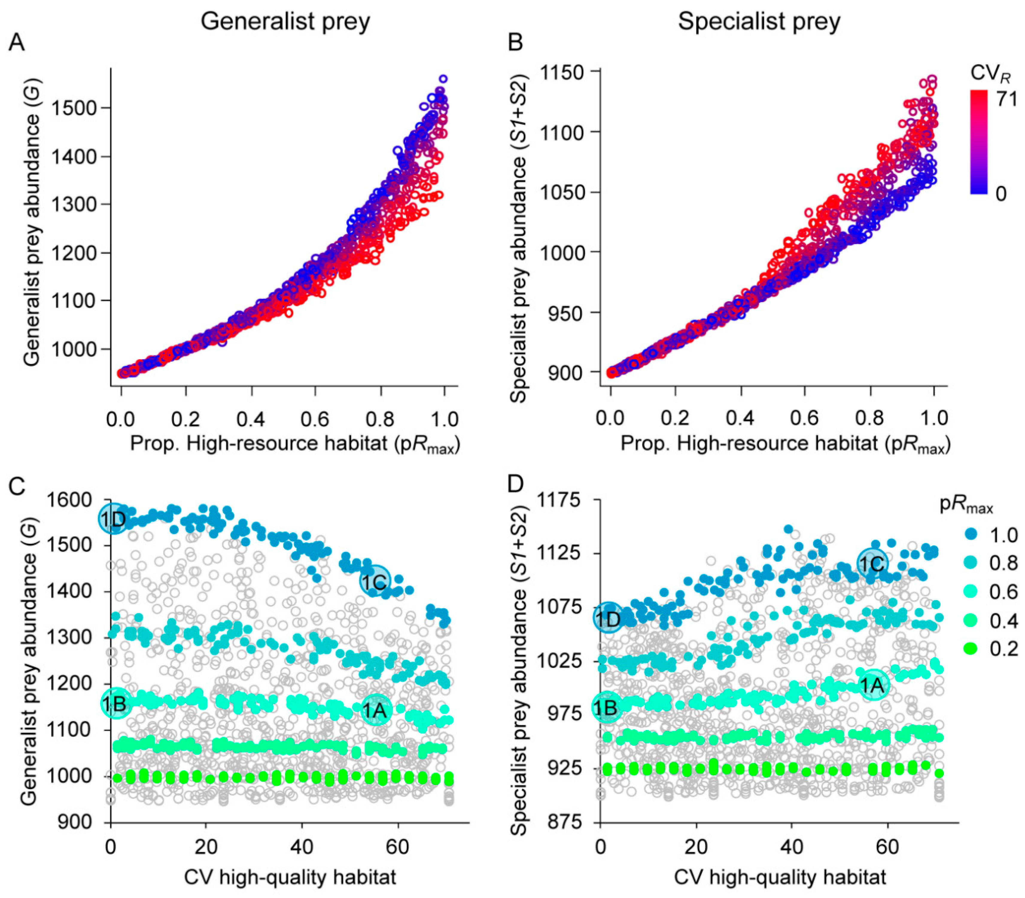
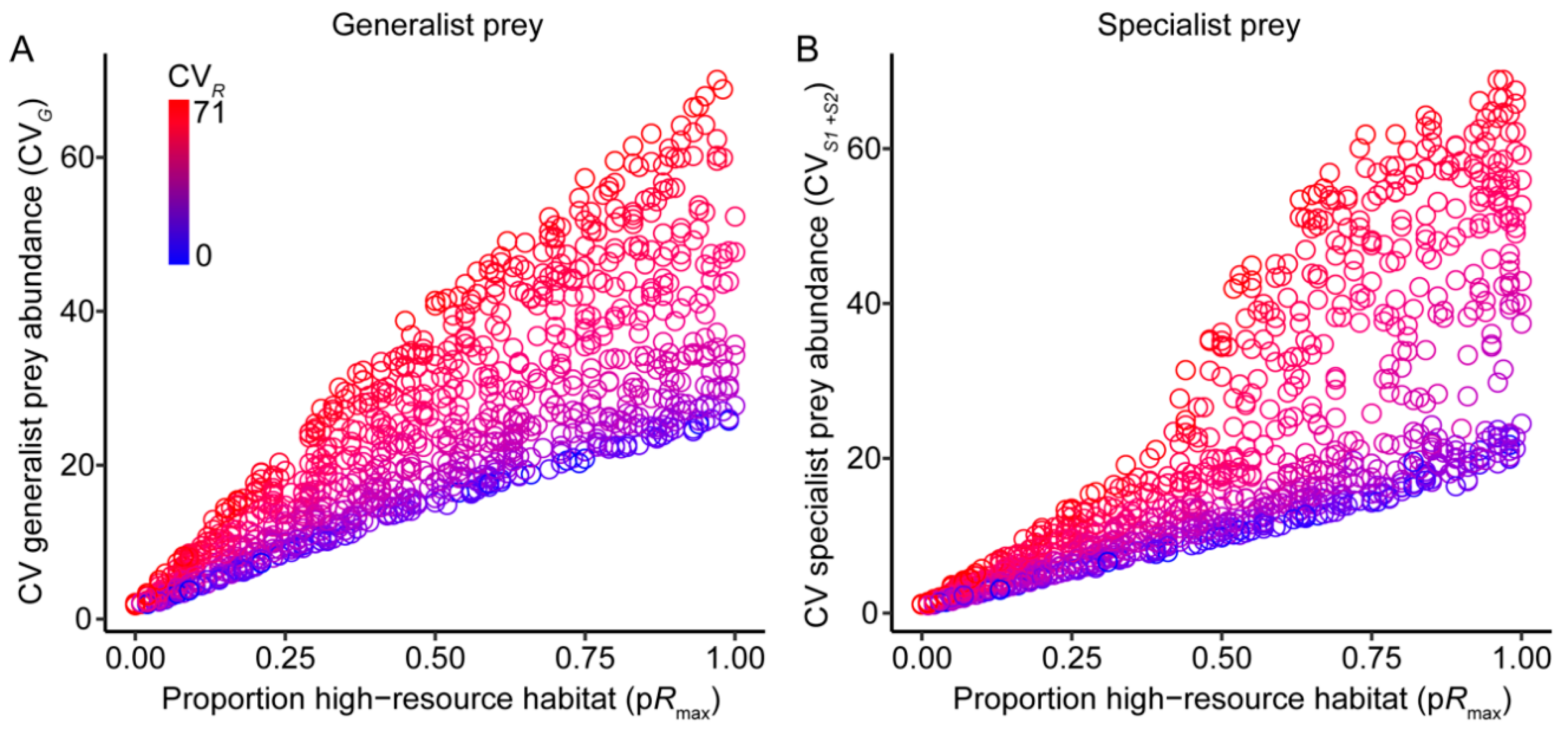
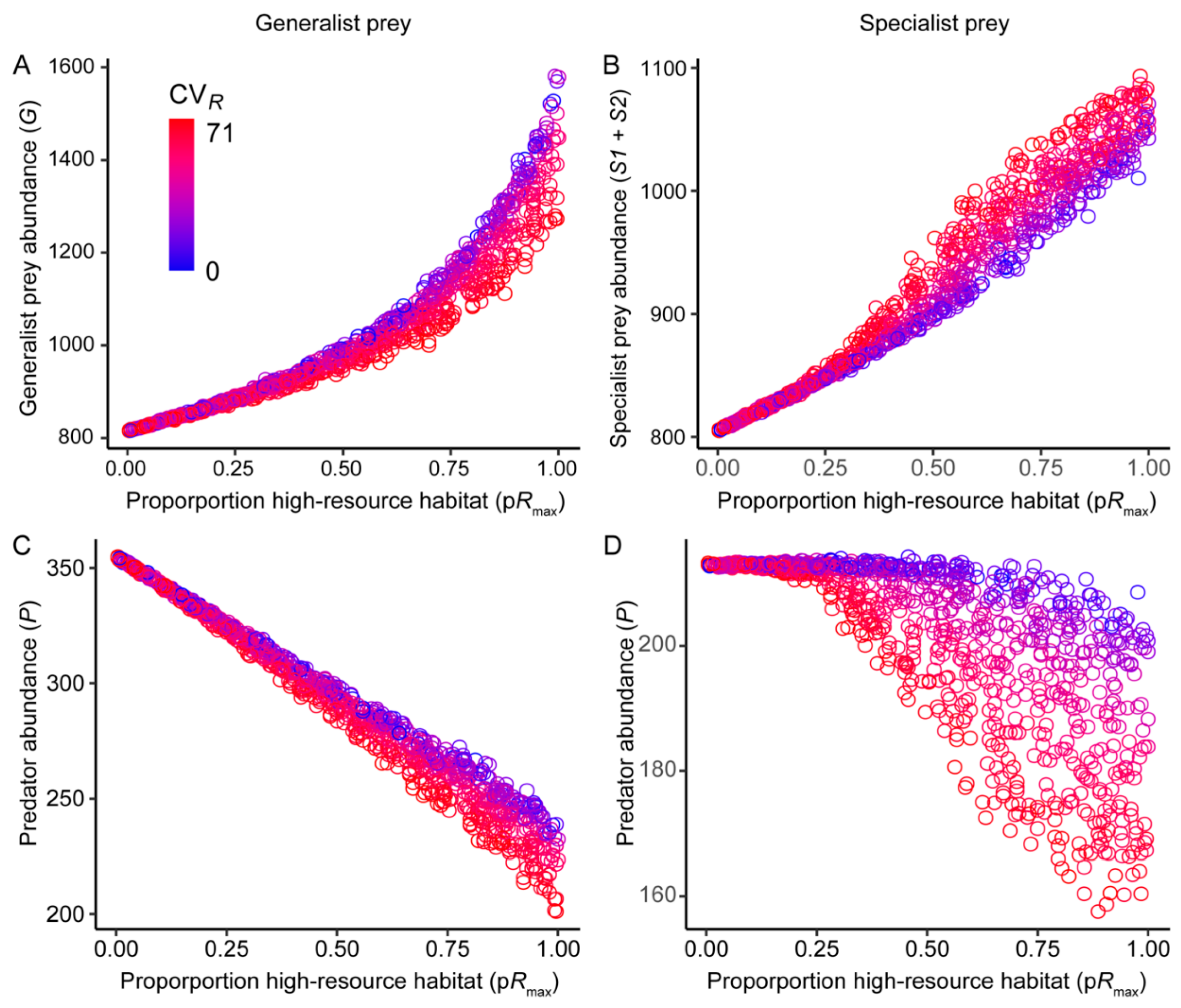
3.1. Effects of Resource Amount and Continuity on Prey

As expected, a greater total (season-long) amount of basal resources in a landscape (R) generally benefited prey populations (Figure 2A,B). The temporal variance of resources (CVR) was also consequential for prey abundance, but this was only evident in high-resource landscapes and the direction of the relationship depended on prey specialization. In landscapes with more high-resource habitat patches (higher levels of pRmax), generalist prey abundance increased as temporal variance decreased (i.e., with greater resource continuity; Figure 2C). The opposite relationship was true in landscapes with two specialist prey, whose summed abundance decreased with lower temporal variance (Figure 2D).

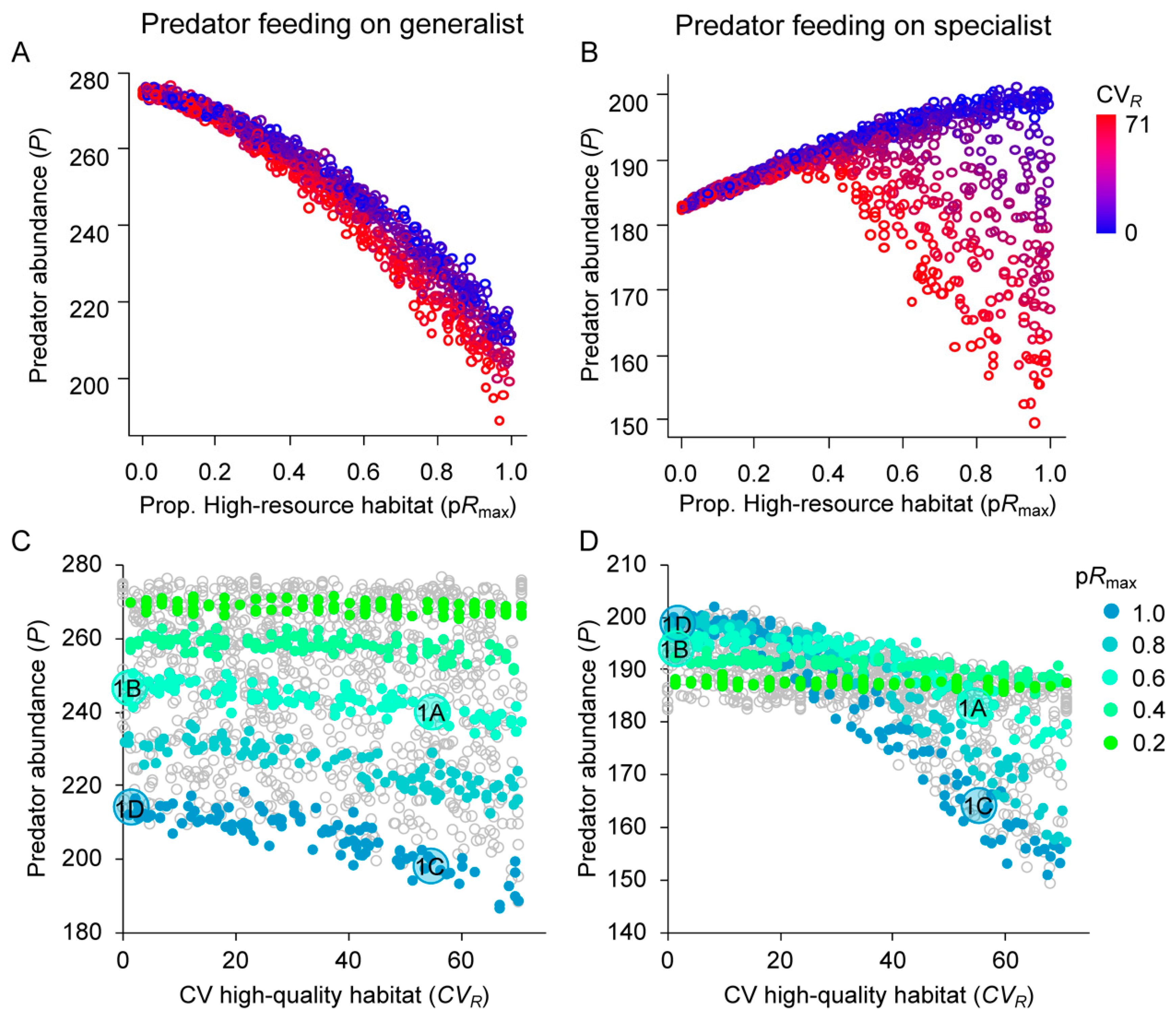
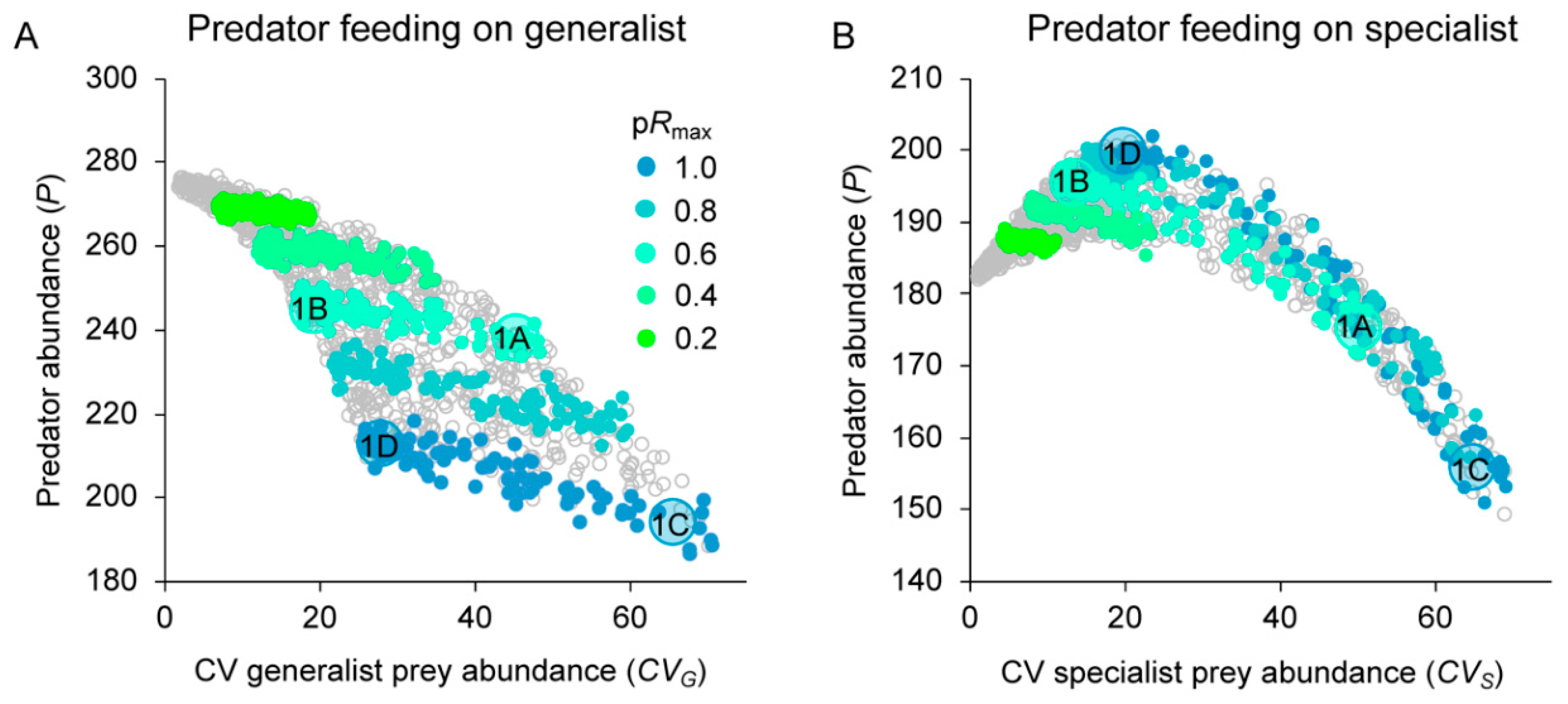
3.2. Effects of Resource Amount and Continuity on Predators

The response of predators to the basal resource amount and temporal variance was similarly dependent on whether prey consisted of a single generalist or two specialist species. When feeding on a single generalist, equilibrium predator abundance counterintuitively decreased with greater total basal resource amount; this was true regardless of basal resource temporal variance (Figure 3A). On the other hand, when feeding on two specialist prey, predator abundance increased with greater resource amount, but only when temporal variance was low (i.e., in landscapes with high resource continuity; Figure 3B, blue points). When temporal variance was high, there was a non-linear relationship between basal resource amount and predator abundance whereby abundance initially increased (i.e., up to pRmax ≈ 0.4), but then decreased (Figure 3B, red points). As with prey, the effects of temporal resource patterns on predator populations were most apparent in high-resource landscapes. Predator abundance generally decreased with greater temporal variance, especially when feeding on specialists (Figure 3C,D).
Given that predators’ responses to basal resource patterns are indirect and mediated by prey, we further investigated the effect of basal resources on the temporal variance of the prey (CVprey; Figure 4) and the direct responses of predators to this prey variance (Figure 5). For both the single generalist and two specialist prey populations, the temporal variability of prey abundance increased with the total resource amount even when basal resources were continuous (i.e., CVR = 0; Figure 4, blue points); basal resource discontinuity exacerbated the effect (Figure 4, red points). Thus, as landscapes filled with more available high-resource patches, and/or when basal resources were available more temporally variable, prey populations cycled with greater amplitude. This is apparent in, for example, metapopulation dynamics, illustrating how both the resource amount (pRmax) and resource temporal variance (CVR) increase prey temporal variance (CVprey) (Figure A2 and Figure A3). The consequence of this high variability in prey abundance was a relative decrease in predator abundance across all levels of basal resource amount (Figure 5).

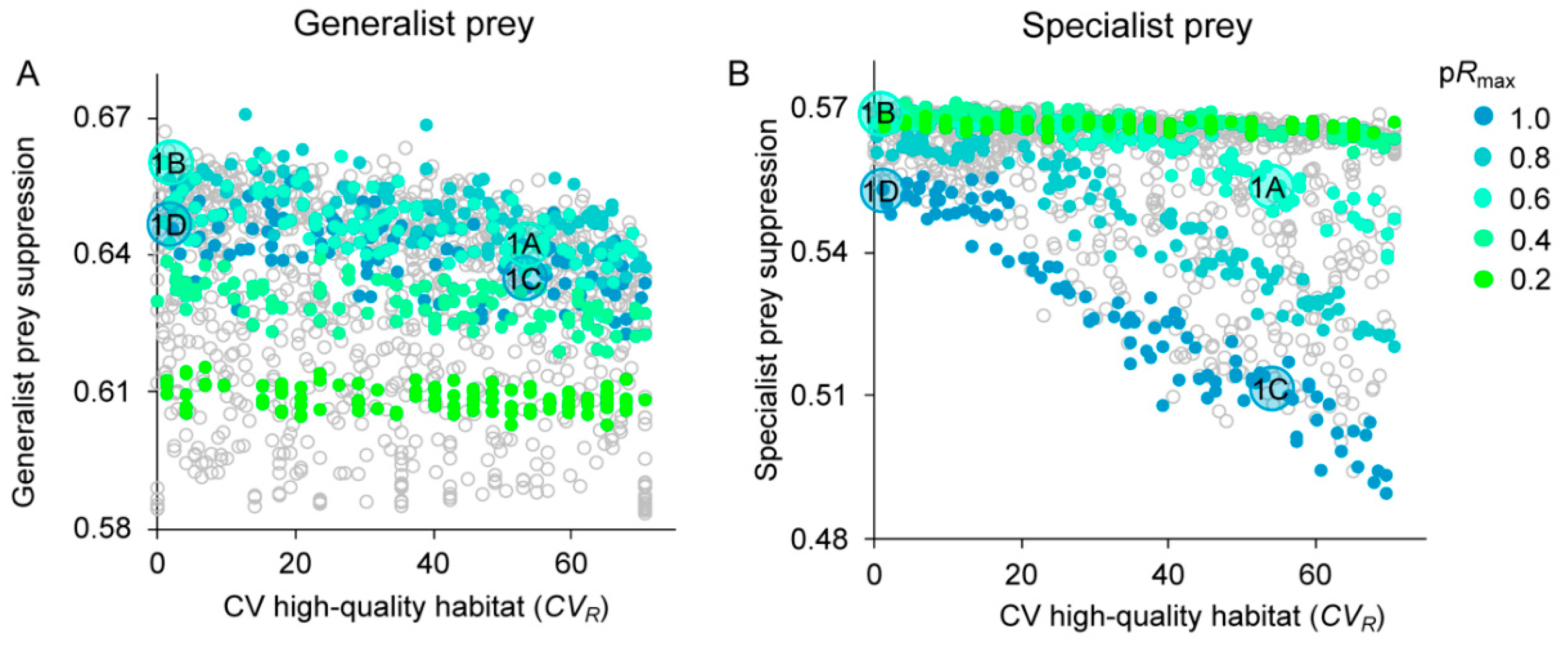
3.3. Prey Suppression

The presence of predators reduced the equilibrium abundance of prey in all model landscapes, but the degree of prey suppression varied with the resource amount and variability (Figure 6). Predator suppression of the single generalist prey species increased with lower temporal variability. This effect was greatest at high levels of habitat in the landscape, with no effect when the resource amount was low (Figure 6A). Generalist prey suppression typically increased with increasing resource amount for all levels of temporal variance.
Suppression of the two specialist prey similarly increased with decreasing temporal variance at high resource levels, and showed no response to temporal variance at low resource levels (Figure 6B). However, the response of specialist prey suppression to resource amount contrasted that of generalist prey suppression, generally decreasing with the increasing resource amount at a given level of temporal variance. Finally, although the rate of suppression of both generalist and specialist prey tended to increase with lower temporal variance (depending on resource amount), this contrasted the relationship between temporal variance and overall predator abundance, which again was negative for the single generalists and positive for the two specialist prey (Figure 2).

4. Discussion

Recent conceptual models have highlighted the importance of incorporating an understanding of the temporal dynamics of resources in a landscape, in addition to total resource amounts, in order to better understand the abundance of organisms [8,9]. Our metapopulation model showed that both the total amount of basal resources in a landscape and the temporal variance of those resources throughout a season can have large and interacting effects on population dynamics of predators and their prey. Altogether, the results suggest that predator abundance, and thus the potential for conservation biological control, is indirectly dependent on the temporal continuity of basal resources in the landscape and not merely the total amount. Furthermore, predator metapopulations and their responses to landscape spatio-temporal dynamics depended on whether prey were comprised of a single generalist or two specialist species.

4.1. Generalist Prey

A key finding of our model was that reduction in the temporal variance of resources at the landscape scale increased resource continuity for both generalist prey and their predators, and thus had a positive effect on abundance when resources were high. Because generalist prey were able to effectively use both early and late season habitats, dispersers had the opportunity to minimize the negative effects of local transition to a low-resource state and disperse to a patch potentially transitioning into a high-resource state. This temporal complementation allowed generalist prey to maintain higher metapopulation sizes even though there were also more predators in the landscape. Low patch connectivity in low-resource landscapes may contribute to this interacting effect; when there were few high-resource patches, dispersal to another one was unlikely even if high-resource patches were present in both halves of the season.
Predators were similarly able to take advantage of a more consistent resource base by dispersing midseason to new and potentially high-resource patches. However, predator abundance declined with the increasing basal resource amount and prey abundance. This type of paradox of enrichment [20] occurs because prey populations become more temporally variable with increasing basal resource amount.
The resulting fluctuations in prey abundance negatively affected predator abundance, outweighing any positive effect of more prey. Although often found in models, the paradox of enrichment is infrequently observed in natural predator–prey systems [21]. This suggests that more empirical research is necessary to explicitly assess the interacting effects of temporal variability and resource amount for predator–prey interactions in agricultural landscapes.

4.2. Specialist Prey

In contrast to the scenario with a single generalist prey species, the summed abundance of two specialist prey species did not increase with lower temporal variance because they were, by design, unable to effectively use alternative resource patches when their preferred resources declined midseason. This meant that specialists could not begin a new generation in a high-resource patch at high abundance through colonization from a patch that was previously in a high-resource state. In effect, specialists were only ever able to have four generations within a growing season (in contrast to generalists’ eight); given the exponential nature of population growth, this put specialists at a disadvantage. Thus, greater temporal variance actually increased the combined equilibrium abundance of two specialist prey species, especially in landscapes high in basal resources (Figure 2C), because specialist prey populations could grow larger while they had the chance. This was compounded by increased predation in low-variance landscapes. Ives and Settle point out that synchronous crop plantings have been promoted to reduce pest outbreaks in tropical rice systems by creating temporal resource gaps for pests, but that this strategy may work only in the absence of predators [15]. Their model agrees with ours in that, in the presence of predators, asynchronous planting (i.e., low-variance landscapes) results in the lowest prey abundance.
When feeding on specialist prey, predators in our model increased in abundance with a greater proportion of high-resource patches in the landscape until about 40%, after which point predator abundance continued to increase only in landscapes with low temporal variance. In these high-resource, low-variance landscapes, the likelihood of resource gaps was sufficiently low such that predators could take advantage of greater abundance of food (prey) without populations becoming destabilized. The heterogeneity of resource availability in low-variance landscapes allows predators to maintain relatively high abundances and move into new patches at densities capable of suppressing prey and preventing rapid prey population growth [22,23]. However, in high-resource, high-variance landscapes, the temporal variance of both generalist and specialist prey was too great to maintain large predator populations.

4.3. Applications to Biological Control and Conservation

More temporally continuous basal resources resulted in higher suppression rates of both a single generalist and two specialist prey in model landscapes. This suggests increased prey suppression (e.g., biological control of pests) in such environments. However, this effect disappeared in landscapes with scarce basal resources, suggesting that enough high-resource patches must be present for temporal variance to be relevant to biological control. A potential reason for this is that, as high-resource patches become increasingly isolated in sparse landscapes, predator dispersal to a high-resource patch becomes increasingly less likely.
However, even though temporally continuity positively affected the rate of prey suppression regardless of prey type, the overall abundance of prey decreased only in the scenario with two specialists, while generalist prey abundance increased. This is a potentially undesirable outcome if the generalist prey is an agricultural pest. However, this situation could be advantageous if the species is not considered a pest [22,24] or if the goal is to conserve biodiversity generally and enhance the populations of both prey and predators [25,26,27].

4.4. Limitations and Future Directions

This study idealizes real-world situations by making multiple simplifying assumptions. For example, the assemblage of plants, herbivores, and natural enemies in real agricultural landscapes is large, overlapping, and complex [28,29]. Future iterations of the model could test various permutations of arthropod communities with different habitat/diet breadths at both trophic levels, or introduce variability in other life history traits of predator and prey species. For example, while the general conclusions of our model were not sensitive to whether prey dispersal was density dependent, other traits such as differences in the spatial scale at which species disperse could be examined. Similarly, vegetation phenologies do not always separate as neatly into early- and late-season resource states as we model here. Thus, additional insights could be gained from new versions of this model that incorporate more complex and diverse patterns of resource phenology in the landscape.
Additionally, our model landscapes did not include habitats that provide locally continuous resources throughout the entire growing season for pest, predators, or both. That is, all high-quality patch states either occurred early, or late, but not both, as may be the case in many agricultural regions. An alternative way of creating landscape-scale resource continuity for mobile consumers would be to retain habitats that provide resources throughout the entire season. These may include perennial crops (e.g., agroforestry systems, perennial grasslands, or pastures) or natural habitats (e.g., forests, prairies, or savannahs). The presence of these habitats would lower temporal variance, which, based on our model results, should increase predator abundance and, in some cases, prey suppression. The greater consistency of resources in such landscapes may contribute to the positive relationships often documented among non-crop area around farm fields, natural enemy populations, and biological control outcomes [2,4].

5. Conclusions

The results of this modeling study support the general hypothesis that temporal discontinuity of resources in a landscape in which mobile consumers forage has a negative effect on their populations [8]. Landscapes with a diverse array of crop and non-crop habitats may provide resources at complementary times of the growing season, which can bolster predator populations and, in some cases, natural pest control. Indeed, recent empirical work on landscape-scale crop heterogeneity has found correlations with biological control [30,31] as well as biodiversity generally across multiple trophic levels [32]. Our model provides evidence for one possible mechanism driving these relationships, namely temporal resource complementation. These results suggest that, through judicious management of habitats in a landscape, either by selecting temporally complementary crops or by managing them for greater asynchrony (e.g., through planned harvest regimes), it is theoretically possible to increase predator population sizes and biological control in some contexts. Furthermore, our model suggests that, in addition to focusing on “habitat amount”, explicitly considering temporal dynamics will be key to understanding how landscape composition influences biodiversity and the ecosystem services.

Supplementary Materials

The following are available online at https://www.mdpi.com/2073-445X/9/12/479/s1, Model codes: specialists code and generalist code.

Author Contributions

Conceptualization, B.S. and C.G.; Formal analysis, B.S.; Funding acquisition, B.S. and C.G.; Investigation, B.S.; Methodology, B.S.; Project administration, C.G.; Supervision, C.G.; Visualization, B.S. and B.I.; Writing—original draft, B.S. and B.I.; Writing—review & editing, B.S., B.I., and C.G. All authors have read and agreed to the published version of the manuscript.

Funding

Support for this research came in part from USDA Grant 2018-67013-28060, the DOE Great Lakes Bioenergy Research Center (DOE BER Office of Science DE-FC02-07ER64494), and DOE OBP Office of Energy Efficiency and Renewable Energy (DE-AC05-76RL01830).

Acknowledgments

We are grateful to Tania Kim, David Hoekman, Tony Ives, and several anonymous reviewers for feedback on earlier manuscript drafts.

Conflicts of Interest

The authors declare no conflict of interest.

Appendix A

Table A1. Model parameter values.
ParameterDefinitionValue
LandscapeRNumber of high-resource patches in the landscape0 to 256
pRmaxProportion of maximum R0 to 1
CVRCoefficient of variation of R
between seasons
Equation (3)
PreyGitGeneralist prey population density in patch i at time tEquation (1)
S1itSpecialist 1 prey population density in patch i at time tEquation (1)
S2itSpecialist 2 prey population density in patch i at time tEquation (1)
SitCombined specialist prey density in patch i at time tS2it + S2it
rPrey intrinsic growth rate1.0
KitPrey carrying capacity in patch i
at time t
100 (xi = 1) or 10 (xi = 0)
mG, S1, or S2Prey mortality rate0.1 or 0.8
dG, S1, or S2Proportion of G, S1, or S2 dispersing from each patch0.2
IitSum of prey immigrating to patch i
at time t
-
EitPrey emigrating from patch i at time t-
CVpreyPrey (G or S) within-season temporal variance (coefficient of variation) Equation (10)
PredatorPitPredator population density in patch i at time tEquations (5) and (6)
cPredator conversion efficiency of prey0.6
aPredator attack rate0.6
mPPredator mortality rate0.1
dPProportion of P dispersing
to new patch
Equations (7) and (8)
IPitSum of predators immigrating to patch i at time t-
EPitPredators emigrating from patch i at time t-
Figure A1. Model runs with predator dispersal set at a fixed rate of 0.2 showing the effects of proportion of high-resource habitat (pRmax) and resource temporal variance (CVR, colored blue-to red) on (A) abundance of a single generalist prey, (B) summed abundance of two specialist prey, (C) predators feeding on a single generalist, and (D) predators feeding on two specialists.
Land 09 00479 g0a1
Figure A2. Example of metapopulation dynamics of the generalist prey (G; green) and predator (P; blue). Landscapes modeled in panels (AD) and associated values of R and CVR correspond to those in Figure 1A–D. For clarity, only the first 100 of 500 generations are shown.
Land 09 00479 g0a2
Figure A3. Example of metapopulation dynamics of the specialist prey (G; green) and predator (P; blue). Landscapes modeled in panels (AD) and associated values of R and CVR correspond to those in Figure 1A–D. For clarity, only the first 100 of 500 generations are shown.
Land 09 00479 g0a3

References

  1. Fahrig, L. Effects of habitat fragmentation on biodiversity. Annu. Rev. Ecol. Evol. Syst. 2003, 34, 487–515. [Google Scholar] [CrossRef] [Green Version]
  2. Dainese, M.; Martin, E.A.; Aizen, M.A.; Albrecht, M.; Bartomeus, I.; Bommarco, R.; Carvalheiro, L.G.; Chaplin-Kramer, R.; Gagic, V.; Garibaldi, L.A.; et al. A global synthesis reveals biodiversity-mediated benefits for crop production. Sci. Adv. 2019, 5, eaax0121. [Google Scholar] [CrossRef] [PubMed] [Green Version]
  3. Kennedy, C.M.; Lonsdorf, E.; Neel, M.C.; Williams, N.M.; Ricketts, T.H.; Winfree, R.; Bommarco, R.; Brittain, C.; Burley, A.L.; Cariveau, D.; et al. A global quantitative synthesis of local and landscape effects on wild bee pollinators in agroecosystems. Ecol. Lett. 2013, 16, 584–599. [Google Scholar] [CrossRef]
  4. Chaplin-Kramer, R.; O’Rourke, M.E.; Blitzer, E.J.; Kremen, C. A meta-analysis of crop pest and natural enemy response to landscape complexity. Ecol. Lett. 2011, 14, 922–932. [Google Scholar] [CrossRef] [PubMed]
  5. Ricketts, T.H.; Regetz, J.; Steffan-Dewenter, I.; Cunningham, S.A.; Kremen, C.; Bogdanski, A.; Gemmill-Herren, B.; Greenleaf, S.S.; Klein, A.M.; Mayfield, M.M.; et al. Landscape effects on crop pollination services: Are there general patterns? Ecol. Lett. 2018, 499–515. [Google Scholar] [CrossRef]
  6. Vasseur, C.; Joannon, A.; Aviron, S.; Burel, F.; Meynard, J.-M.; Baudry, J. The cropping systems mosaic: How does the hidden heterogeneity of agricultural landscapes drive arthropod populations? Agric. Ecosyst. Environ. 2013, 166, 3–14. [Google Scholar] [CrossRef]
  7. Cohen, A.L.; Crowder, D.W. The impacts of spatial and temporal complexity across landscapes on biological control: A review. Curr. Opin. Insect Sci. 2017, 20, 13–18. [Google Scholar] [CrossRef] [Green Version]
  8. Schellhorn, N.A.; Gagic, V.; Bommarco, R. Time will tell: Resource continuity bolsters ecosystem services. Trends Ecol. Evol. 2015, 30, 524–530. [Google Scholar] [CrossRef]
  9. Iuliano, B.; Gratton, C. Temporal resource (dis)continuity for conservation biological control: From field to landscape scales. Front. Sustain. Food Syst. 2020, 4. [Google Scholar] [CrossRef]
  10. Dunning, J.B.; Danielson, B.J.; Pulliam, H.R. Ecological processes that affect populations in complex landscapes. Oikos 1992, 65, 169–175. [Google Scholar] [CrossRef] [Green Version]
  11. Mallinger, R.E.; Gibbs, J.; Gratton, C. Diverse landscapes have a higher abundance and species richness of spring wild bees by providing complementary floral resources over bees’ foraging periods. Landsc. Ecol. 2016, 31, 1523–1535. [Google Scholar] [CrossRef]
  12. Rundlöf, M.; Persson, A.S.; Smith, H.G.; Bommarco, R. Late-season mass-flowering red clover increases bumble bee queen and male densities. Biol. Conserv. 2014, 172, 138–145. [Google Scholar] [CrossRef]
  13. Mandelik, Y.; Winfree, R.; Neeson, T.; Kremen, C. Complementary habitat use by wild bees in agro-natural landscapes. Ecol. Appl. 2012, 22, 1535–1546. [Google Scholar] [CrossRef] [PubMed]
  14. Levins, R. Some Demographic and Genetic Consequences of Environmental Heterogeneity for Biological Control. Bull. Entomol. Soc. Am. 1969, 15, 237–240. [Google Scholar] [CrossRef]
  15. Ives, A.R.; Settle, W.H. Metapopulation dynamics and pest control in agricultural systems. Am. Nat. 1997, 149, 220–246. [Google Scholar] [CrossRef]
  16. Bianchi, F.J.J.A.; Van der Werf, W. Model evaluation of the function of prey in non-crop habitats for biological control by ladybeetles in agricultural landscapes. Ecol. Model. 2004, 171, 177–193. [Google Scholar] [CrossRef]
  17. Le Gal, A.; Robert, C.; Accatino, F.; Claessen, D.; Lecomte, J. Modelling the interactions between landscape structure and spatio-temporal dynamics of pest natural enemies: Implications for conservation biological control. Ecol. Model. 2020, 420, 108912. [Google Scholar] [CrossRef]
  18. Taylor, A.D. Metapopulations, Dispersal, and Predator-Prey Dynamics: An Overview. Ecology 1990, 71, 429–433. [Google Scholar] [CrossRef]
  19. Holling, C.S. Some characteristics of simple types of predation and parasitism. Can. Entomol. 1959, 91, 385–398. [Google Scholar] [CrossRef]
  20. Rosenzweig, M.L. Paradox of Enrichment: Destabilization of Exploitation Ecosystems in Ecological Time. Science 1971, 171, 385–387. [Google Scholar] [CrossRef]
  21. Jensen, C.X.J.; Ginzburg, L.R. Paradoxes or theoretical failures? The jury is still out. Ecol. Model. 2005, 188, 3–14. [Google Scholar] [CrossRef]
  22. Settle, W.H.; Ariawan, H.; Astuti, E.T.; Cahyana, W.; Hakim, A.L.; Hindayana, D.; Lestari, A.S. Managing tropical rice pests through conservation of generalist natural enemies and alternative prey. Ecology 1996, 77, 1975–1988. [Google Scholar] [CrossRef]
  23. Holt, R.D. Population dynamics in two-patch environments: Some anomalous consequences of an optimal habitat distribution. Theor. Popul. Biol. 1985, 28, 181–208. [Google Scholar] [CrossRef]
  24. Harwood, J.D.; Obrycki, J.J. The role of alternative prey in sustaining predator populations. In Proceedings of the Second International Symposium on Biological Control of Arthropods, Davos, Switzerland, 12–16 September 2005; pp. 453–462. [Google Scholar]
  25. Harvey, J.A.; Heinen, R.; Armbrecht, I.; Basset, Y.; Baxter-Gilbert, J.H.; Bezemer, T.M.; Böhm, M.; Bommarco, R.; Borges, P.A.V.; Cardoso, P.; et al. International scientists formulate a roadmap for insect conservation and recovery. Nat. Ecol. Evol. 2020, 4, 174–176. [Google Scholar] [CrossRef]
  26. Bercovitch, F.B. Conservation conundrum: Endangered predators eating endangered prey. Afr. J. Ecol. 2018, 56, 434–435. [Google Scholar] [CrossRef] [Green Version]
  27. Roemer, G.W.; Wayne, R.K. Conservation in Conflict: The Tale of Two Endangered Species. Conserv. Biol. 2003, 17, 1251–1260. [Google Scholar] [CrossRef]
  28. Vandermeer, J.; Armbrecht, I.; de la Mora, A.; Ennis, K.K.; Fitch, G.; Gonthier, D.J.; Hajian-Forooshani, Z.; Hsieh, H.-Y.; Iverson, A.; Jackson, D.; et al. The Community Ecology of Herbivore Regulation in an Agroecosystem: Lessons from Complex Systems. BioScience 2019, 69, 974–996. [Google Scholar] [CrossRef] [Green Version]
  29. Snyder, W.E. Give predators a complement: Conserving natural enemy biodiversity to improve biocontrol. Biol. Control 2019, 135, 73–82. [Google Scholar] [CrossRef]
  30. Redlich, S.; Martin, E.A.; Steffan-Dewenter, I. Landscape-level crop diversity benefits biological pest control. J. Appl. Ecol. 2018, 55, 2419–2428. [Google Scholar] [CrossRef]
  31. Bosem-Baillod, A.; Tscharntke, T.; Clough, Y.; Batáry, P. Landscape-scale interactions of spatial and temporal cropland heterogeneity drive biological control of cereal aphids. J. Appl. Ecol. 2017, 54, 1804–1813. [Google Scholar] [CrossRef] [Green Version]
  32. Sirami, C.; Gross, N.; Baillod, A.B.; Bertrand, C.; Carrié, R.; Hass, A.; Henckel, L.; Miguet, P.; Vuillot, C.; Alignier, A.; et al. Increasing crop heterogeneity enhances multitrophic diversity across agricultural regions. Proc. Natl. Acad. Sci. USA 2019, 116, 16442–16447. [Google Scholar] [CrossRef] [PubMed] [Green Version]
Figure 1. Conceptual diagrams (left) and corresponding model landscapes (right) for landscapes with different proportions of high-resource habitat (pRmax) and temporal variance (CVR). Gray lines represent the amount of resources provided by early-season habitat (gray patches). Black lines represent the amount of resources provided by late-season habitat (black patches). White patches provide consistently few basal resources year-round. Panels (AD) show model landscapes with different patterns of resource amount and continuity.
Land 09 00479 g001
Figure 2. Prey response to the amount (pRmax, top panels) and variability (CVR, bottom panels) of high-resource habitat in the landscape. Left panels (A,C) show the response of a single generalist prey, G. Right panels (B,D) show the sum of the density response of two specialist prey, S1 + S2. Points represent individual model runs with landscapes varying across parameter space. Labels (1A–1D) within panels C and D indicate model runs corresponding to the landscapes shown in Figure 1.
Land 09 00479 g002
Figure 3. Predator response to the amount (pRmax, top panels) and variability (CVR, bottom panels) of high-resource habitat in the landscape. Left panels (A,C) show the response of predators feeding on a single generalist prey. Right panels (B,D) show the response of predators feeding on two specialist prey. Points represent individual model runs with landscapes varying across parameter space. Labels (circles 1A–1D) within panels (C,D) indicate model runs corresponding to the landscapes shown in Figure 1.
Land 09 00479 g003
Figure 4. Variability in the abundance of (A) generalist and (B) summed specialist prey changes with increasing proportion of high-resource habitat (pRmax) in the landscape and greater temporal variance in R (CVR, color-coded blue to red).
Land 09 00479 g004
Figure 5. Predator response to variation in prey (CVprey) when feeding on (A) one generalist prey species G and (B) two specialist prey S1 + S2. Colors indicate the proportion of patches with maximum resource amount (pRmax), or the amount of the landscape providing high-resource habitat, for each of 100 separate model runs. Gray points represent a set of 1000 model runs where pRmax was randomly selected between 0 and 1. Labels (circles 1A–1D) indicate model runs corresponding to the landscapes shown in Figure 1.
Land 09 00479 g005
Figure 6. Suppression of (A) generalist and (B) specialist prey in response to changing temporal variance of basal resources (CVR). Colors indicate the proportion of patches maximum resource amount (pRmax), or the amount of the landscape providing high-resource habitat, for each of 100 separate model runs. Gray points represent a set of 1000 model runs where pRmax was randomly selected between 0 and 1. Labels (circles 1A–D) indicate model runs corresponding to the landscapes shown in Figure 1.
Land 09 00479 g006
Publisher’s Note: MDPI stays neutral with regard to jurisdictional claims in published maps and institutional affiliations.

