Characterizing the Landscape Structure of Urban Wetlands Using Terrain and Landscape Indices

Abstract
:1. Introduction
2. Materials and Methods
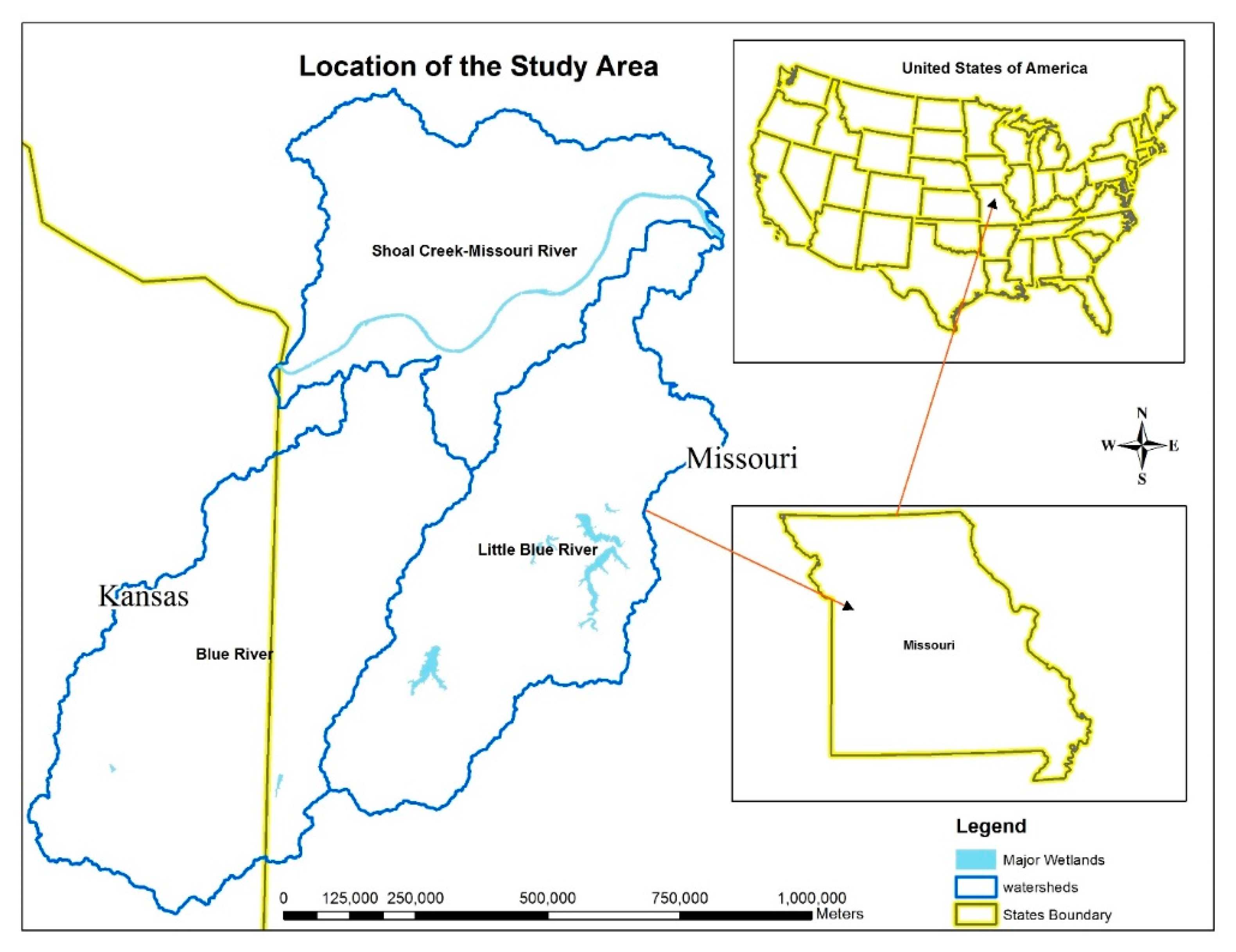
2.1. Study Area
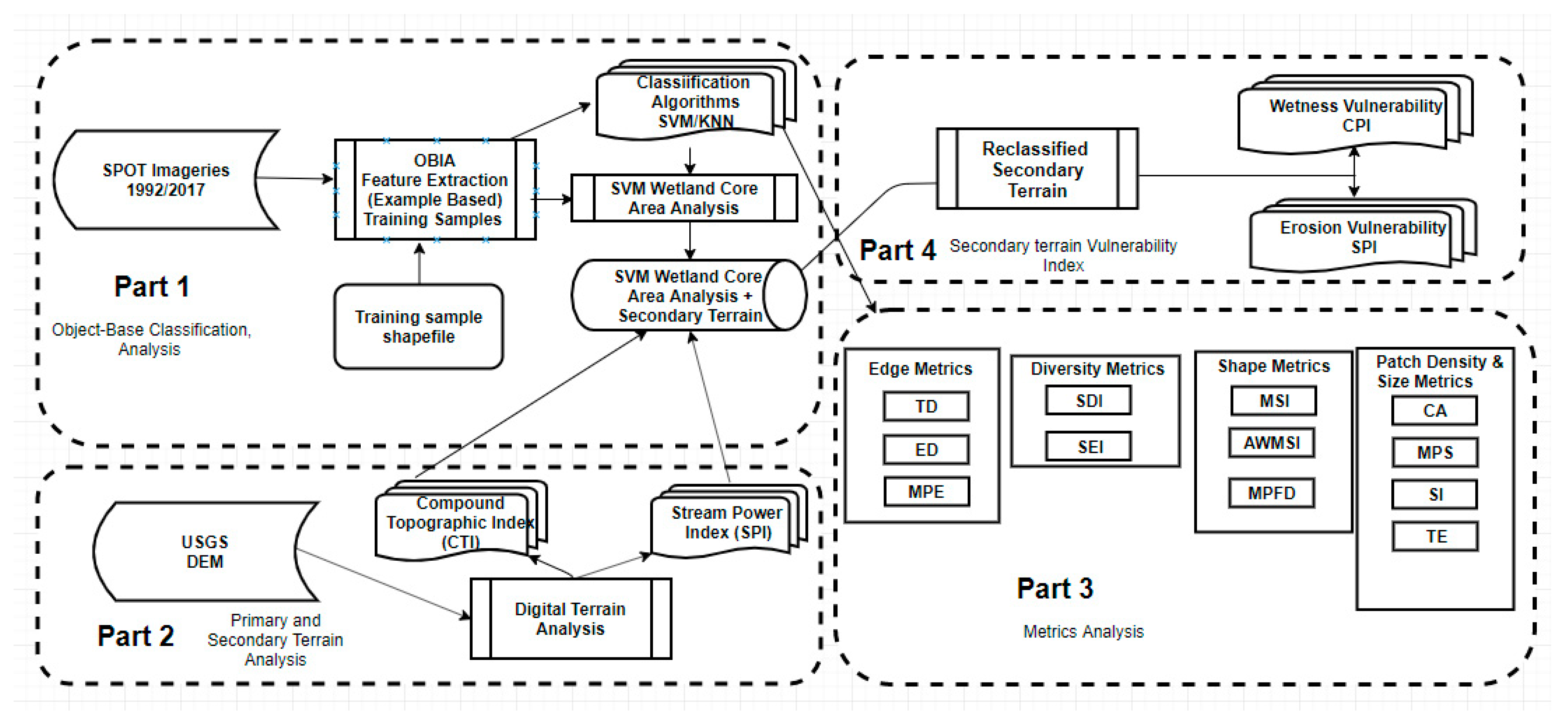
2.2. Methods
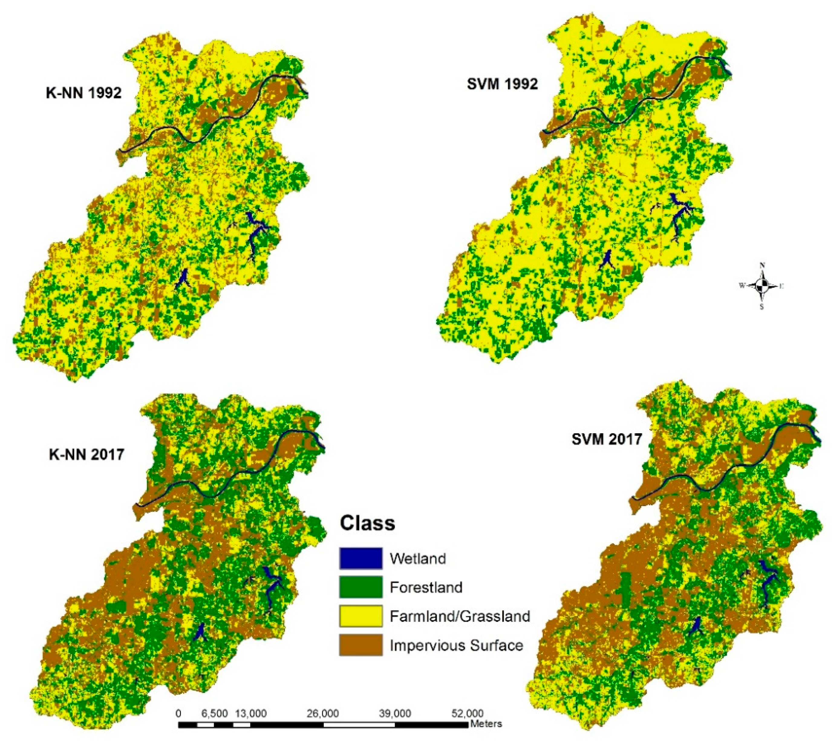
2.2.1. Image Classification Techniques
2.2.2. Classification Scheme
2.2.3. Accuracy Assessment
2.2.4. Terrain Analysis
- Ln represents natural logarithm;
- A represents the catchment area per pixel;
- β refers to the slope in degrees.
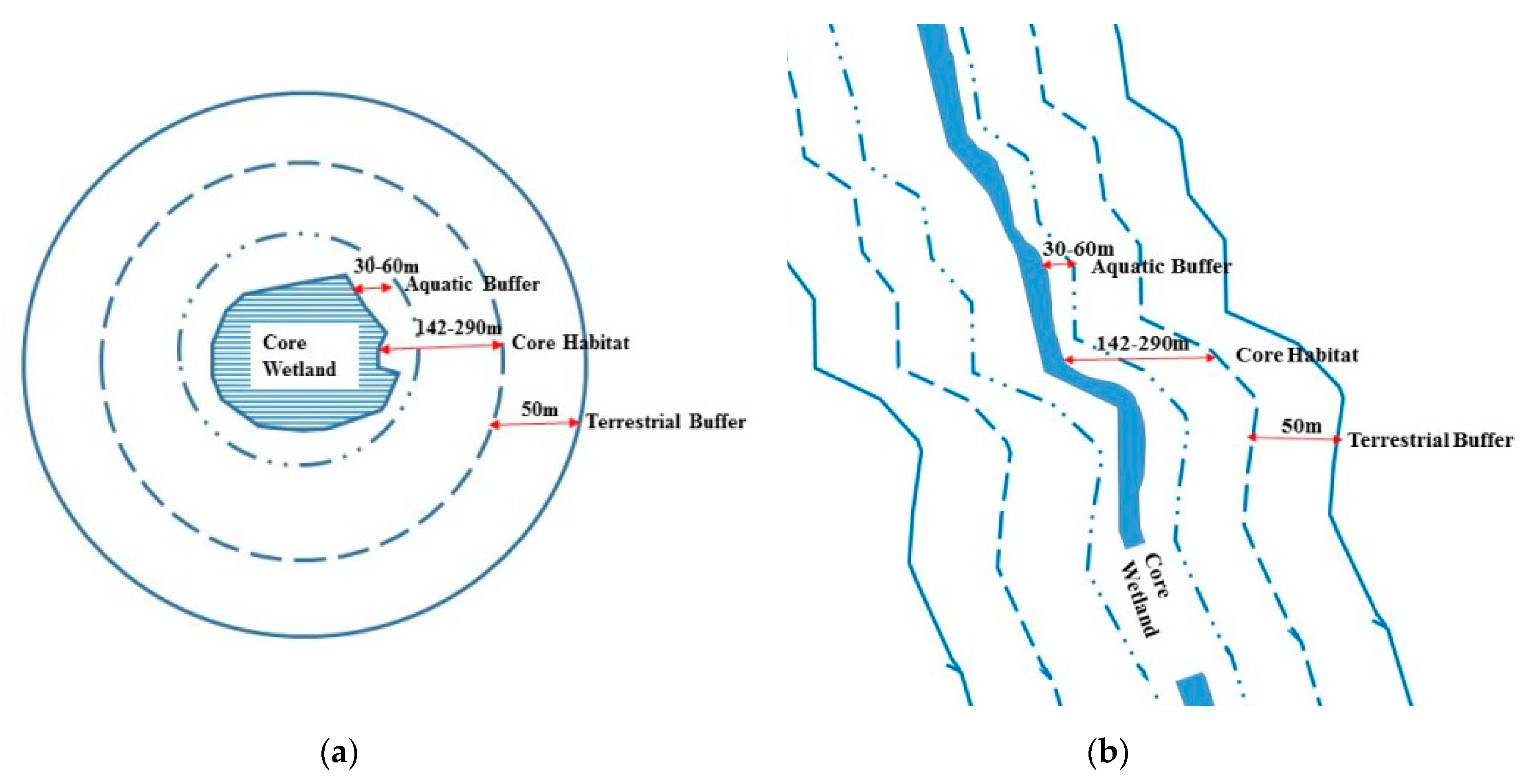
2.2.5. Urban Wetland Terrestrial Habitat Buffer
- %ΔvE—percentage change in vulnerability estimate;
- —wetness area for CTI;
- —stream power area for SPI;
- —non-wetness area for CTI;
- —non-stream power area for SPI.
2.2.6. Landscape Metrics Calculations
3. Results
3.1. Landscape Level Analysis
3.1.1. Change Detection Statistics (CDS)
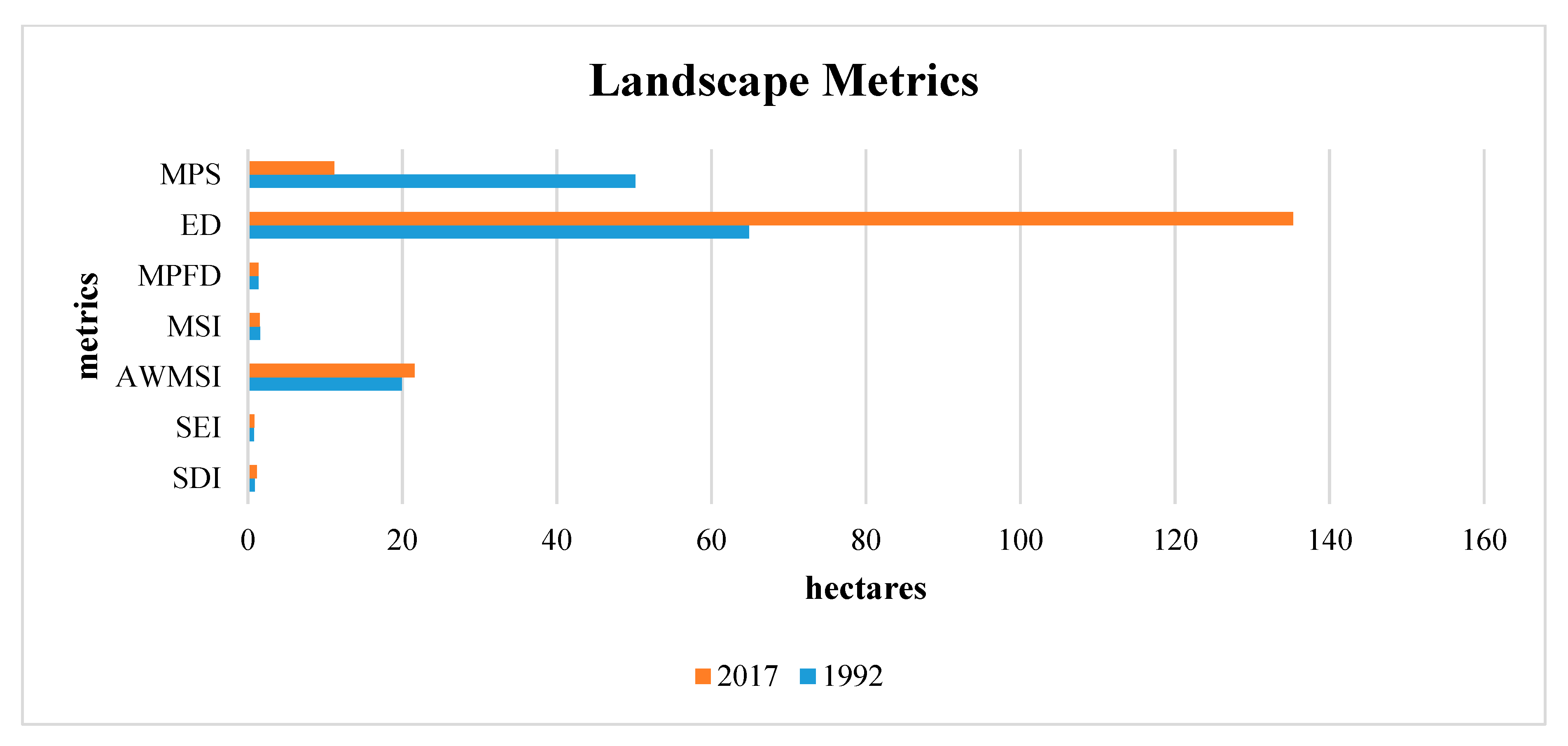
3.1.2. Landscape Level Metric Calculation
3.2. Wetland-Level Analysis
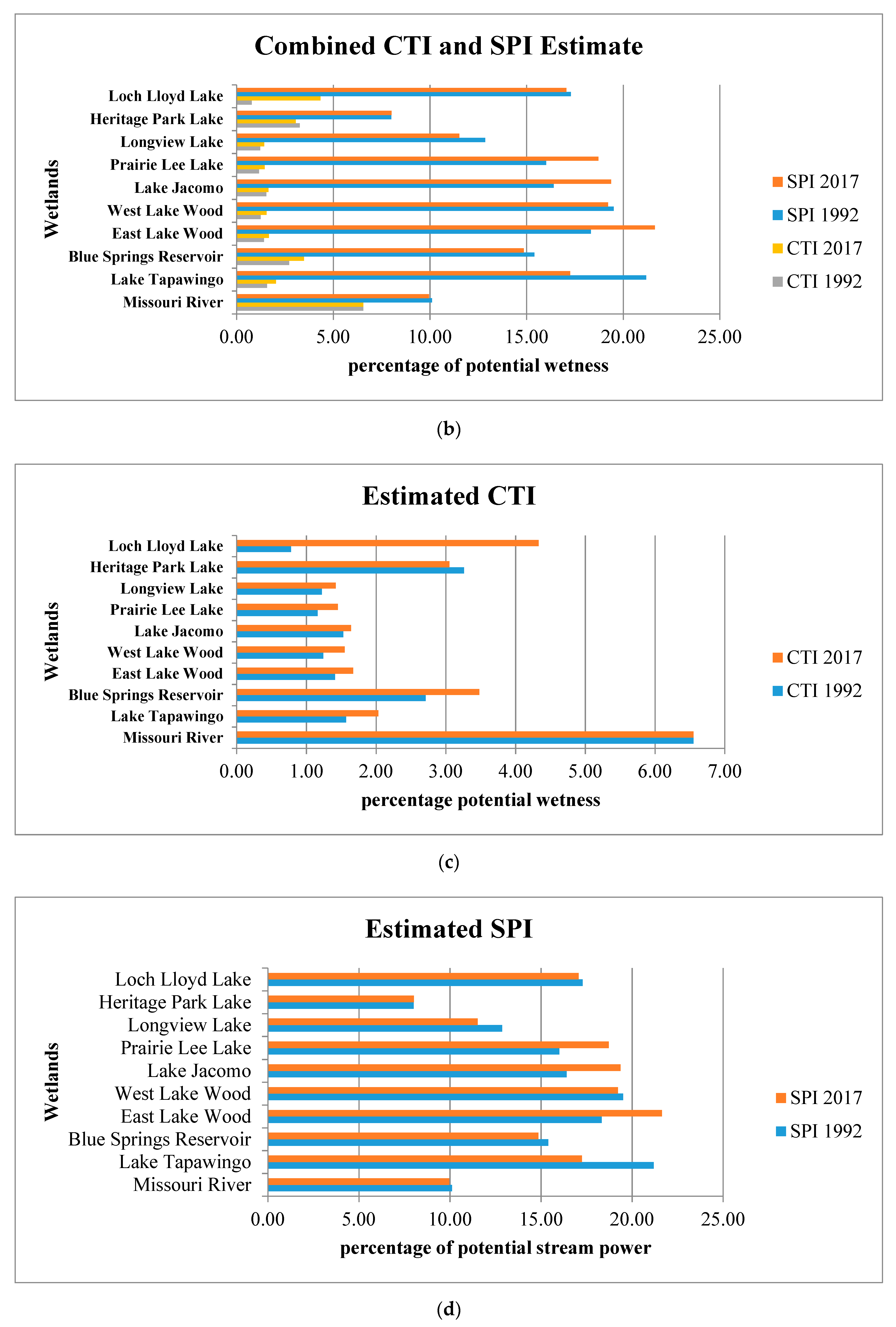
3.2.1. Terrain Calculation
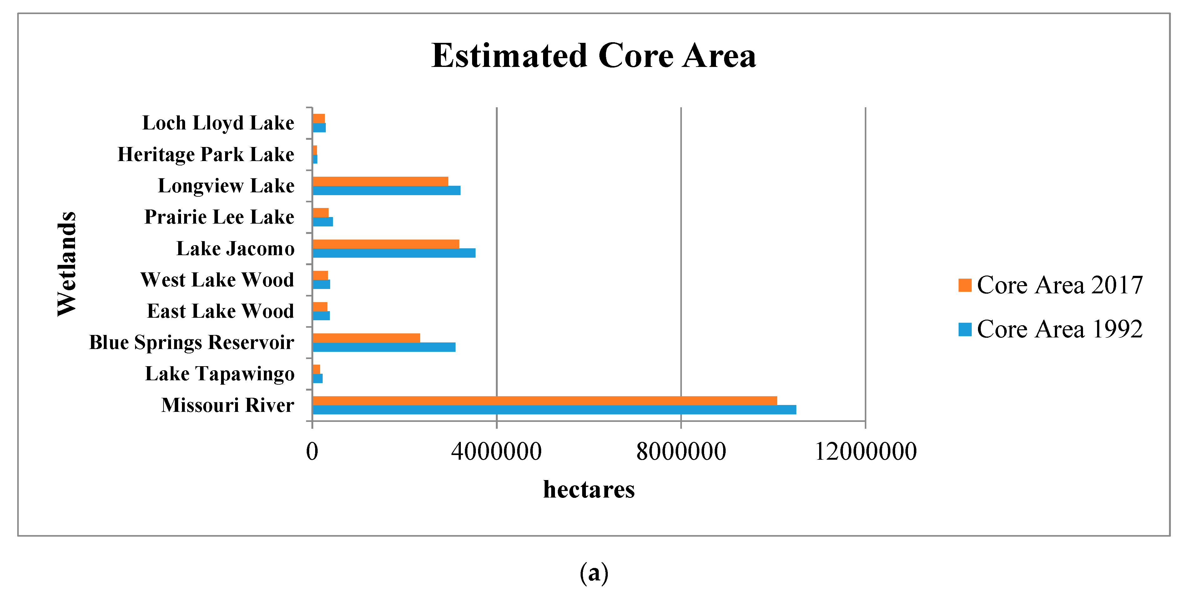
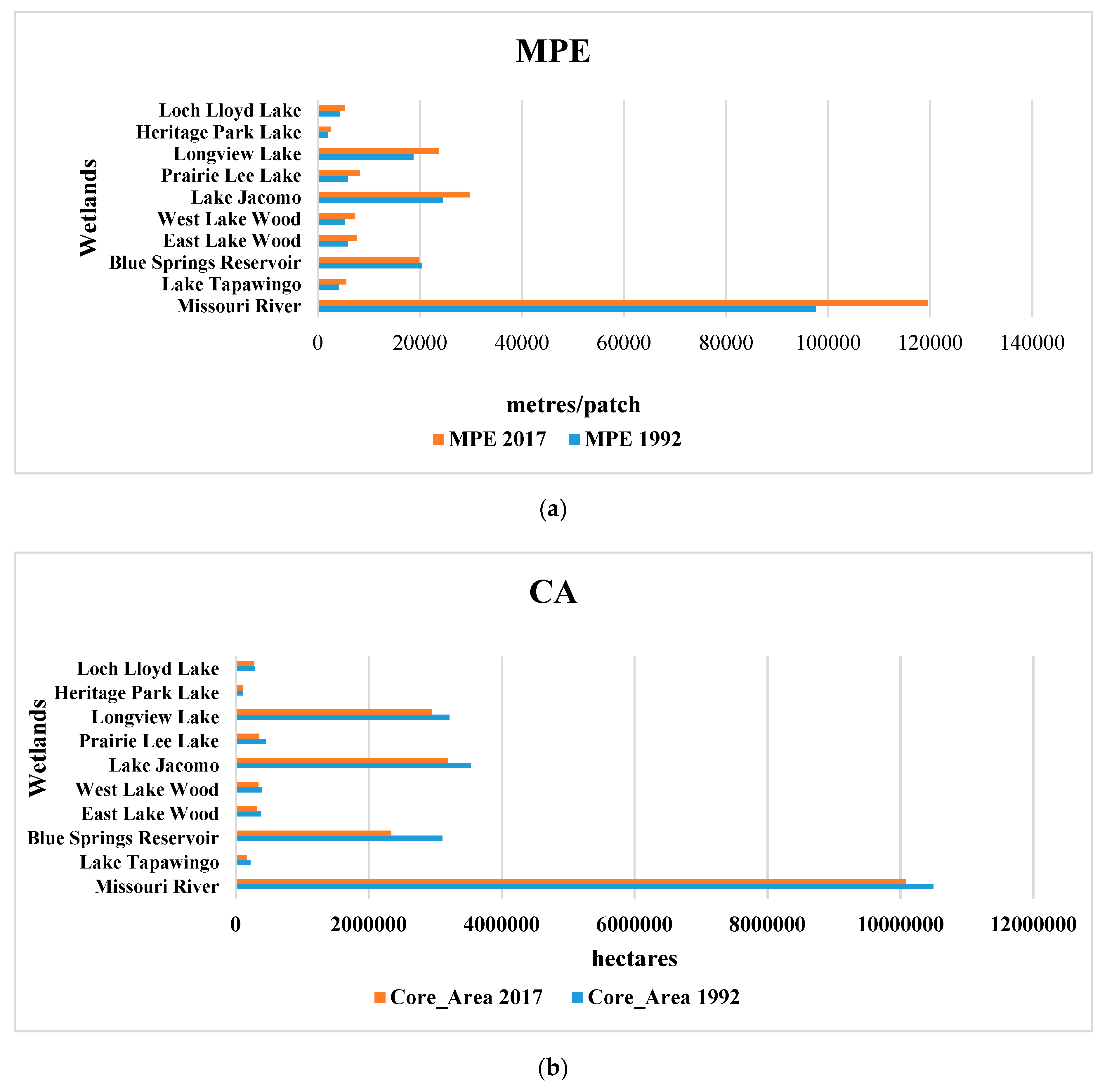
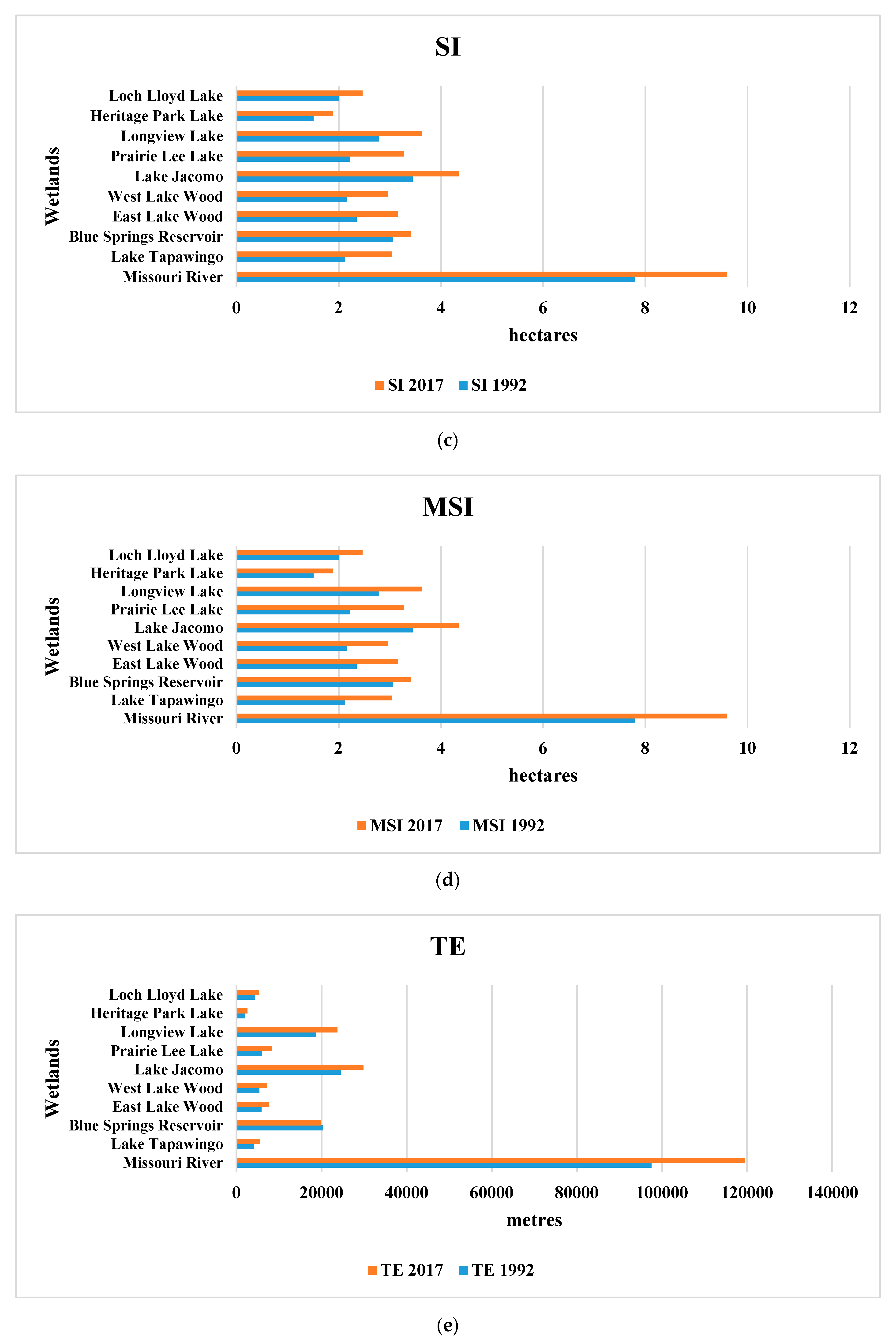
3.2.2. Patch Level Metric Calculation
4. Discussion
5. Conclusions
Author Contributions
Funding
Conflicts of Interest
Appendix A

| Compound Topographical Index Estimate | ||
| 1992 | 2017 | Wetland Impact |
 |  | Blue Springs Reservoir Estimated CTI 1992 = 2.71% 2017 = 3.48% |
 |  | East Lake Wood Estimated CTI 1992 = 1.41% 2017 = 1.67% |
 |  | Heritage Park Lak Estimated CTI 1992 = 3.26% 2017 = 3.10% |
| Compound Topographical Index Estimate | ||
| 1992 | 2017 | Wetland Impact |
 |  | Lake Jacomo Estimated CTI 1992 = 1.53% 2017 = 1.64% |
 |  | Loch Lloyd Lake Estimated CTI 1992 = 0.78% 2017 = 4.33% |
 |  | Longview Lake Estimated CTI 1992 = 1.22% 2017 = 1.42% |
 |  | Lake Tapawingo Estimated CTI 1992 = 1.57% 2017 = 2.03% |
| Compound Topographical Index Estimate | ||
| 1992 | 2017 | Wetland Impact |
 |  | Missouri River Estimated CTI 1992 = 6.55% 2017 = 6.55% |
 |  | Prairie Lee Lake Estimated CTI 1992 = 1.16% 2017 = 1.45% |
 |  | West Lake Wood Estimated CTI 1992 = 1.24% 2017 = 1.55% |
Appendix B
| Stream Power Index Estimate | ||
| 1992 | 2017 | Wetland Impact |
 |  | Blue Springs Reservoir Estimated SPI 1992 = 15.40% 2017 = 14.85% |
 |  | East Lake Wood Estimated SPI 1992 = 18.33% 2017 = 21.64% |
 |  | Heritage Park Lake Estimated SPI 1992 = 8.00% 2017 = 8.01% |
| Stream Power Index Estimate | ||
| 1992 | 2017 | Wetland Impact |
 |  | Lake Jacomo Estimated SPI 1992 = 16.40% 2017 = 19.37% |
 |  | Loch Lloyd Lake Estimated SPI 1992 = 17.29% 2017 = 17.06% |
 |  | Longview Lake Estimated SPI 1992 = 12.86% 2017 = 11.52% |
| Stream Power Index Estimate | ||
| 1992 | 2017 | Wetland Impact |
 |  | Lake Tapawingo Estimated SPI 1992 = 21.19% 2017 = 17.25% |
 |  | Missouri River Estimated SPI 1992 = 10.11% 2017 = 9.95% |
 |  | Prairie Lee Lake Estimated SPI 1992 = 16.01 %2017 = 18.72 |
 |  | West Lake Wood Estimated SPI 1992 = 19.51% 2017 = 19.22% |
References
- Ji, W. Remotely-Sensed Urban Wet-Landscapes: An Indicator of Coupled Effects of Human Impact and Climate Change. Int. Arch. Photogramm. Remote. Sens. Spat. Inf. Sci. 2016, 915. [Google Scholar] [CrossRef] [Green Version]
- Dale, V.H.; Brown, S.; Haeuber, R.A.; Hobbs, N.T.; Huntly, N.; Naiman, R.J.; Riebsame, W.E.; Turner, M.G.; Valone, T.J. Ecological principles and guidelines for managing the use of the land. In The Ecological Design and Planning Reader; Island Press: Washington, DC, USA, 2014; pp. 279–298. [Google Scholar]
- Li, H.; Franklin, J.F.; Swanson, F.J.; Spies, T.A. Developing alternative forest cutting patterns: A simulation approach. Landsc. Ecol. 1993, 8, 63–75. [Google Scholar] [CrossRef]
- Harding, J.S.; Benfield, E.F.; Bolstad, P.V.; Helfman, G.S.; Jones, E.B.D. Stream biodiversity: The ghost of land use past. Proc. Natl. Acad. Sci. USA 1998, 95, 14843–14847. [Google Scholar] [CrossRef] [PubMed] [Green Version]
- Wang, X.; Blanchet, F.G.; Koper, N. Measuring habitat fragmentation: An evaluation of landscape pattern metrics. Methods Ecol. Evol. 2014, 5, 634–646. [Google Scholar] [CrossRef]
- Zubair, O.; Ji, W.; Weilert, T. Modeling the impact of urban landscape change on urban wetlands using similarity weighted instance-based machine learning and Markov model. Sustainability 2017, 9, 2223. [Google Scholar] [CrossRef] [Green Version]
- Kelly, M.; Blanchard, S.D.; Kersten, E.; Koy, K. Terrestrial remotely sensed imagery in support of public health: New avenues of research using object-based image analysis. Remote. Sens. 2011, 3, 2321–2345. [Google Scholar] [CrossRef] [Green Version]
- Ji, W.; Ma, J.; Twibell, R.W.; Underhill, K. Characterizing urban sprawl using multi-stage remote sensing images and landscape metrics. Comput. Environ. Urban Syst. 2006, 30, 861–879. [Google Scholar] [CrossRef]
- Weilert, T.; Ji, W.; Zubair, O. Assessing the Impacts of Streamside Ordinance Protection on the Spatial and Temporal Variability in Urban Riparian Vegetation. ISPRS Int. J. Geoinf. 2018, 7, 282. [Google Scholar] [CrossRef] [Green Version]
- McGarigal, K. Introduction to Landscape Ecology. Duke University. 2000. Available online: http://www.umass.edu/landeco/about/landeco.pdf (accessed on 24 December 2019).
- Turner, M.G.; Gardner, R.H.; O’neill, R.V.; O’Neill, R.V. Landscape Ecology in Theory and Practice; Springer: New York, NY, USA, 2001; Volume 401. [Google Scholar]
- Moody, A.; Woodcock, C.E. The influence of scale and the spatial characteristics of landscapes on land-cover mapping using remote sensing. Landsc. Ecol. 1995, 10, 363–379. [Google Scholar] [CrossRef]
- Li, F.; Wang, R.; Hu, D.; Ye, Y.; Yang, W.; Liu, H. Measurement methods and applications for beneficial and detrimental effects of ecological services. Ecol. Indic. 2014, 47, 102–111. [Google Scholar] [CrossRef]
- Turner, M.G.; O’Neill, R.V.; Gardner, R.H.; Milne, B.T. Effects of changing spatial scale on the analysis of landscape pattern. Landsc. Ecol. 1989, 3, 153–162. [Google Scholar] [CrossRef]
- Peña-Barragán, J.M.; Ngugi, M.K.; Plant, R.E.; Six, J. Object-based crop identification using multiple vegetation indices, textural features and crop phenology. Remote. Sens. Environ. 2011, 115, 1301–1316. [Google Scholar] [CrossRef]
- Liu, J.; Linderman, M.; Ouyang, Z.; An, L.; Yang, J.; Zhang, H. Ecological degradation in protected areas: The case of Wolong Nature Reserve for giant pandas. Science 2001, 292, 98–101. [Google Scholar] [CrossRef] [Green Version]
- Semlitsch, R.D. Biological delineation of terrestrial buffer zones for pond-breeding salamanders. Conserv. Biol 1998, 12, 1113–1119. [Google Scholar] [CrossRef]
- Semlitsch, R.D.; Jensen, J.B. Core habitat, not buffer zone. Natl. Wetl. Newsl. 2001, 23, 5–6. [Google Scholar]
- Hartman, G.F.; Scrivener, J.C.E. Impacts of forestry practices on a coastal stream ecosystem, Carnation Creek, British Columbia. Can. Bull. Fish. Aquat. Sci. 1990, 223, 148. [Google Scholar]
- Davies, P.E.; Nelson, M. Relationships between riparian buffer widths and the effects of logging on stream habitat, invertebrate community composition and fish abundance. Mar. Freshw. Res. 1994, 45, 1289–1305. [Google Scholar] [CrossRef]
- Brosofske, K.D.; Chen, J.; Naiman, R.J.; Franklin, J.F. Harvesting effects on microclimatic gradients from small streams to uplands in western Washington. Ecol. Appl. 1997, 7, 1188–1200. [Google Scholar] [CrossRef]
- Weller, D.E.; Jordan, T.E.; Correll, D.L. Heuristic models for material discharge from landscapes with riparian buffers. Ecol. Appl. 1998, 8, 1156–1169. [Google Scholar] [CrossRef]
- Keller, C.M.; Robbins, C.S.; Hatfield, J.S. Avian communities in riparian forests of different widths in Maryland and Delaware. Wetlands 1993, 13, 137–144. [Google Scholar] [CrossRef]
- McComb, W.C.; McGarigal, K.; Anthony, R.G. Small mammal and amphibian abundance in streamside and upslope habitats of mature Douglas-fir stands, western Oregon. Northwest Sci. 1993, 67, 181. [Google Scholar]
- Darveau, M.; Beauchesne, P.; Belanger, L.; Huot, J.; Larue, P. Riparian forest strips as habitat for breeding birds in boreal forest. J. Wildl. Manag. 1995, 59, 67–78. [Google Scholar] [CrossRef]
- Hodges, M.F., Jr.; Krementz, D.G. Neotropical migratory breeding bird communities in riparian forests of different widths along the Altamaha River, Georgia. Wilson Bull. 1996, 108, 496–506. [Google Scholar]
- Semlitsch, R.D. Principles for management of aquatic breeding amphibians. J. Wildl. Manag. 2000, 64, 615–631. [Google Scholar] [CrossRef]
- Bodie, J.R. Stream and riparian management for freshwater turtles. J. Environ. Manag. 2001, 62, 443–455. [Google Scholar] [CrossRef]
- Darveau, M.; Labbé, P.; Beauchesne, P.; Bélanger, L.; Huot, J. The use of riparian forest strips by small mammals in a boreal balsam fir forest. For. Ecol. Manag. 2001, 143, 95–104. [Google Scholar] [CrossRef]
- Spackman, S.C.; Hughes, J.W. Assessment of minimum stream corridor width for biological conservation: Species richness and distribution along mid-order streams in Vermont, USA. Biol. Conserv. 1995, 71, 325–332. [Google Scholar] [CrossRef]
- Cushman, S.A.; McGarigal, K.; Neel, M.C. Parsimony in landscape metrics: Strength, universality and consistency. Ecol. Indic. 2008, 8, 691–703. [Google Scholar] [CrossRef]
- Tomaselli, V.; Tenerelli, P.; Sciandrello, S. Mapping and quantifying habitat fragmentation in small coastal areas: A case study of three protected wetlands in Apulia (Italy). Environ. Monit. Assess. 2012, 184, 693–713. [Google Scholar] [CrossRef]
- McGarigal, K.; Cushman, S.; Regan, C. Quantifying Terrestrial Habitat Loss and Fragmentation. A Protocol. Available online: http://www.umass.edu/landeco/teaching/landscape_ecology/labs/fragprotocol.pdf (accessed on 10 January 2019).
- Saura, S.; Martinez-Millan, J. Sensitivity of landscape pattern metrics to map spatial extent. Photogramm. Eng. Remote. Sens. 2001, 67, 1027–1036. [Google Scholar]
- MARC (Mid-America Regional Council). Census Data for the MARC Region. Available online: https://www.marc.org/Data-Economy/Maps-and-GIS (accessed on 20 November 2019).
- Zubair, O.A.; Ji, W.; Festus, O. Urban Expansion and the Loss of Prairie and Agricultural Lands: A Satellite Remote-Sensing-Based Analysis at a Sub-Watershed Scale. Sustainability 2019, 11, 4673. [Google Scholar] [CrossRef] [Green Version]
- Jensen, J.R. Introductory Digital Image Processing: A Remote Sensing Perspective; Prentice Hall Press: Upper Saddle River, NJ, USA, 2015; pp. 501–548. [Google Scholar]
- Yu, Q.; Gong, P.; Clinton, N.; Biging, G.; Kelly, M.; Schirokauer, D. Object-based detailed vegetation classification with airborne high spatial resolution remote sensing imagery. Photogramm. Eng. Remote. Sens. 2006, 72, 799–811. [Google Scholar] [CrossRef] [Green Version]
- O’Neill, R.V.; Hunsaker, C.T.; Jones, K.B.; Riitters, K.H.; Wickham, J.D.; Schwartz, P.M.; Goodman, I.A.; Jackson, B.L.; Baillargeon, W.S. Monitoring environmental quality at the landscape scale: Using landscape indicators to assess biotic diversity, watershed integrity, and landscape stability. BioScience 1997, 47, 513–519. [Google Scholar] [CrossRef] [Green Version]
- L3 Harris Geospatial Documentation Center. Available online: https://www.harrisgeospatial.com/docs/using_envi_Home.html (accessed on 24 December 2019).
- United State Geological Services (USGS) 3DEP Product Metadata. Available online: https://www.usgs.gov/core-science-systems/ngp/ss/3dep-product-metadata (accessed on 24 December 2019).
- Timm, D. Identifying Critical Source Areas for Best Management Practice Targeting in Impaired Zumbro River Watersheds Using Digital Terrain Analysis. Master’s Thesis, University of Minnesota, Twin Cities, MN, USA, 2016. [Google Scholar]
- Wilson, J.P.; Gallant, J.C. Terrain Analysis: Principles and Applications; Wilson, J.P., Gallant, J.C., Eds.; John Wiley & Sons: New York, NY, USA, 2000. [Google Scholar]
- Murcia, C. Edge effects in fragmented forests: Implications for conservation. Trends Ecol. Evol. 1995, 10, 58–62. [Google Scholar] [CrossRef]
- Semlitsch, R.D.; Bodie, J.R. Biological criteria for buffer zones around wetlands and riparian habitats for amphibians and reptiles. Conserv. Biol. 2003, 17, 1219–1228. [Google Scholar] [CrossRef] [Green Version]
- Lu, D.; Weng, Q. A survey of image classification methods and techniques for improving classification performance. Int. J. Remote. Sens. 2007, 28, 823–870. [Google Scholar] [CrossRef]
- McGarigal, K. Landscape Metrics for Categorical Map Patterns. Lecture Notes. Available online: http://www.umass.edu/landeco/teaching/landscape_ecology/schedule/chapter9_metrics.pdf (accessed on 3 July 2018).
- Hansen, A.J.; Risser, P.G.; di Castri, F. Epilogue: Biodiversity and ecological flows across ecotones. In Landscape Boundaries; Springer: New York, NY, USA, 1992; pp. 423–438. [Google Scholar]
- Temple, S.A. Predicting Impacts of Habitat Fragmentation on Forest Birds: A Comparison of Two Models; Lewis Publishers: New York, NY, USA, 1986. [Google Scholar]
- Öckinger, E.; Schweiger, O.; Crist, T.O.; Debinski, D.M.; Krauss, J.; Kuussaari, M.; Petersen, J.D.; Poyry, J.; Settele, J.; Summerville, K.S.; et al. Life-history traits predict species responses to habitat area and isolation: A cross-continental synthesis. Ecol. Lett. 2010, 13, 969–979. [Google Scholar] [CrossRef]
- Liu, G.; Zhang, L.; Zhang, Q.; Musyimi, Z.; Jiang, Q. Spatio–temporal dynamics of wetland landscape patterns based on remote sensing in Yellow River Delta, China. Wetlands 2014, 34, 787–801. [Google Scholar] [CrossRef]
- Kolozsvary, M.B.; Swihart, R.K. Habitat fragmentation and the distribution of amphibians: Patch and landscape correlates in farmland. Can. J. Zool. 1999, 77, 1288–1299. [Google Scholar] [CrossRef]


| Class Name Description | Class Name Description |
|---|---|
| Wetlands (WL) | Rivers, lakes, ponds, riparian area, vegetated depressions |
| Farmland/Grassland(FGL) | Cultivated land, grasslands, golf courses, lawns |
| Impervious surfaces (IS) | Built-up areas (buildings, roads, paved walk-ways, etc.) |
| Forestland (FL) | Trees and shrubs |
| Confusion Matrix: Accuracy of Object-Oriented Classification Results | ||||||||
|---|---|---|---|---|---|---|---|---|
| SPOT Image | Supervised Classification Method | Overall Accuracy (%) | Overall Kappa Coefficient | Ground Truth Wetland (%) | Prod. Acc. (%) | User Acc. (%) | Commission (%) | Omission (%) |
| 1992 | SVM | 63.84 | 0.48 | 96.75 | 96.75 | 92.25 | 7.75 | 3.25 |
| K-NN | 61.42 | 0.45 | 96.75 | 96.75 | 93.20 | 6.80 | 3.25 | |
| 2017 | SVM | 89.14 | 0.80 | 95.86 | 97.29 | 94.91 | 6.26 | 4.14 |
| K-NN | 79.54 | 0.65 | 97.29 | 95.86 | 93.74 | 5.09 | 2.71 | |
| Acronym | Name (Units) | Description | Justification |
|---|---|---|---|
| TCAI | Total Core Area Index (ha) | Total core area index is a measure of the amount of core area in the patch or landscape | Fragmentation |
| SI | Shape index (ha) | normalized ratio of patch perimeter to area | Fragmentation |
| CA | Core Area (ha) | The total size of disjunct core patches (hectares). | Fragmentation |
| ED | edge density (m/ha) | Amount of edge relative to the landscape area | Fragmentation |
| TE | Total edge (m) | Perimeter of patches | Fragmentation |
| MPE | Mean Patch Edge (m/patch) | Average amount of edge per patch | Fragmentation |
| MPS | Mean Patch Size (ha) | Mean Patch Size of Patches (Class or Landscape Level) | Fragmentation |
| MSI | Mean Shape Index (ha) | sum of each patch’s perimeter divided by the square root of patch area (in hectares) | Fragmentation |
| AWMSI | Area Weighted Mean Shape Index (ha) | AWMSI equals the sum of each patch’s perimeter, divided by the square root of patch area (in hectares) | Fragmentation |
| MPFD | Mean Patch Fractal Dimension (ha) | Measure shape Complexity | Fragmentation |
| SDI | Shannon’s Diversity Index (ha) | Measure of relative patch diversity | Diversity |
| SEI | Shannon’s Evenness Index (ha) | Measure of patch distribution and abundance | Diversity |
| Initial State | ||||
|---|---|---|---|---|
| Final State | Wetland (%) | Row Total (%) | Class Total (%) | |
| Wetland | 82.18 | 99.91 | 100.00 | |
| Class Total | 100.00 | 100.00 | 100.00 | |
| Class Changes | 17.82 | |||
| Image Difference | 9.17 | |||
| Initial State | ||||
|---|---|---|---|---|
| Final State | Wetland (%) | Row Total (%) | Class Total (%) | |
| Wetland | 79.00 | 99.81 | 100.00 | |
| Class Total | 100.00 | 100.00 | 100.00 | |
| Class Changes | 21.00 | |||
| Image Difference | 8.08 | |||
© 2020 by the authors. Licensee MDPI, Basel, Switzerland. This article is an open access article distributed under the terms and conditions of the Creative Commons Attribution (CC BY) license (http://creativecommons.org/licenses/by/4.0/).
Share and Cite
O. Festus, O.; Ji, W.; Zubair, O.A. Characterizing the Landscape Structure of Urban Wetlands Using Terrain and Landscape Indices. Land 2020, 9, 29. https://doi.org/10.3390/land9010029
O. Festus O, Ji W, Zubair OA. Characterizing the Landscape Structure of Urban Wetlands Using Terrain and Landscape Indices. Land. 2020; 9(1):29. https://doi.org/10.3390/land9010029
Chicago/Turabian StyleO. Festus, Olusola, Wei Ji, and Opeyemi A. Zubair. 2020. "Characterizing the Landscape Structure of Urban Wetlands Using Terrain and Landscape Indices" Land 9, no. 1: 29. https://doi.org/10.3390/land9010029