Extracting Features from Satellite Imagery to Understand the Size and Scale of Housing Sub-Markets in Madrid

Abstract

The following paper proposes a novel machine learning approach to the segmentation of urban housing markets. We extract features from globally available satellite imagery using an unsupervised machine learning model called MOSAIKS, and apply a k-means clustering algorithm to the extracted features to identify sub-markets at multiple intra-urban scales within a case study of Madrid (Spain). To systematically explore scale effects on the resulting clusters, the analysis is repeated with varying sizes of satellite image patches. We assess the resulting clusters across scales using several internal cluster-evaluation metrics. Additionally, we use data from online listings portal Idealista to measure the homogeneity of housing prices within the clusters, to understand how well sub-markets can be differentiated by the image features. This paper evaluates the strengths and weakness of the method to identify urban housing sub-markets, a task which is important for planners and policy makers and is often limited by a lack of data. We conclude that the approach seems useful to divide large urban housing markets according to different attributes and scales.

1. Introduction

The spatial structure of house prices within urban areas is a key driver of socio-economic inequalities and segregation [1,2]. Differences in house prices and housing price appreciation rates between neighbourhoods further exacerbates wealth and access inequality [3]. Despite the impact of spatial house price differentials on urban inequality, the majority of research on housing market dynamics has focused on the macro scale. Recently this has begun to change, in part due to the increasing availability of micro geocoded datasets of dwellings, their characteristics, and prices [4].

The availability of micro-level datasets and other new forms of data provides new opportunities for measuring urban land use including urban residential patterns. Housing sub-markets, segments of homogenous housing which are heterogenous between one another, are central to how we understand a single large urban housing market. A plethora of studies agree that it is preferable to divide a unitary housing market into smaller sub-markets [5,6,7,8]. Sub-markets are commonly understood as areas with similar housing prices, housing characteristics, and neighbourhood attributes [9,10].

Delineating a large and spatially heterogenous housing market into disaggregated units improves the predictive accuracy of hedonic house price models [11], which typically regress house prices against structural, neighbourhood and accessibility features [12]. These models are useful for house price prediction, understanding the drivers of housing prices and testing the effects of market shocks or policies on prices. Using housing delineations in hedonic models improves the model fit by reducing the spatial dependence in housing prices and characteristics [13,14]. Aggregating similar properties into groups also allows the effect of different attributes on prices to vary across market segments; for example, the effect of having a good school on housing prices is likely to be stronger in a neighbourhood with mostly families than retirees.

Sub-markets also provide a useful framework for policy makers, planners, and real estate actors to explore neighbourhood housing market dynamics and improve decision making [15]. Additionally, sub-markets provide a framework to monitor changes to the structure of local housing markets over time. So far, very little is known about how housing sub-markets change [16,17,18]. Capturing sub-markets and their temporal changes would allow us to receive a better understanding of price movements between neighbourhoods and the resulting impact on segregation and inequality in cities.

However, the Modifiable Area Unit Problem (MAUP) means that statistical bias can be created when point data are aggregated into spatial units, due to the scale at which the aggregations are created and how the boundaries are drawn [19]. Census delineations or other types of neighbourhood boundaries are commonly used to segment local housing markets. Their use likely introduces the MAUP if they are not representative of the spatial characteristics of the housing market [15]. These delineations are also not updated frequently, so may become outdated as populations and the housing sub-markets shift over time [20].

Despite much scholarly attention over several decades, how to best define housing sub-markets, conceptually and empirically, remains a topic of contention. Spatial heterogeneity, spatial dependence, and spatial scale are central to the spatial organization of housing submarkets [12,21]. Appropriate modelling of spatial heterogeneity, the variation in features across locations, depends on the choice of scale. The scale of sub-markets can range from national or regional, through to metropolitan areas to below the metropolitan level, down to the street scale [22]. The most appropriate scale is the one that minimises spatial dependence in prices, as changing the scale alters the geographic patterns of housing and neighbourhood characteristics [23]. The ‘best’ scale at which to model housing-market dynamics is locally specific and depends on the variable(s) used to assess the homogeneity of the sub-markets.

Quantitative methods used to delineate sub-markets and segment housing fall into two main groups: hedonic models and clustering algorithms [24]. Clustering has been shown to be an effective means of sub-market delineation. These algorithms group observations based on many highly dimensional variables, including structural housing characteristics, demographic and socio-economic variables, and distances to different amenities. K-means is one example of a clustering algorithms used for housing market segmentation [5,14,25]. Other algorithms applied more recently to submarket delineation include fuzzy c-means [26], density based spatial clustering [27], and probabilistic hierarchical clustering approach using a Bayesian network [28]. Clustering, however, requires vast amounts of individual-level housing data which is costly to acquire and often not available over time. Our methodology advances beyond traditional clustering methods by using processed satellite imagery as the input to the clustering algorithm.

Methodological advances in machine learning and Artificial Intelligence have created new opportunities to monitor spatial patterns in urban morphology from large datasets [29,30]. In the last ten years, the open availability of increasingly higher-resolution satellite imagery through user-friendly online platforms such as Microsoft’s Planetary Hub, as well as cloud computing, has made this type of big data easier to process and analyse [31]. Convolutional Neural Networks (CNN) have been shown as successful for feature extraction tasks. For example, a convolutional autoencoder, a neural network model designed for learning encodings of input data, has been employed to identify neighbourhoods from latent image features in Sentinel 2 satellite data [32]. The authors note that exploring the scale effects on these models requires more research.

With an application to housing, street view, satellite imagery and neural networks have been used to measure micro-level features of the urban environment [33]; features such as visual desirability have been shown to improve house price prediction [34]. Similarly, research has shown that features from satellite imagery of wider areas around housing samples improved the accuracy of house-price prediction [35]. To the best of our knowledge, with the exception of a couple of similar studies which identify neighbourhoods using features extracted from satellite imagery [32,36,37], this kind of imagery has not been employed to delineate housing sub-markets.

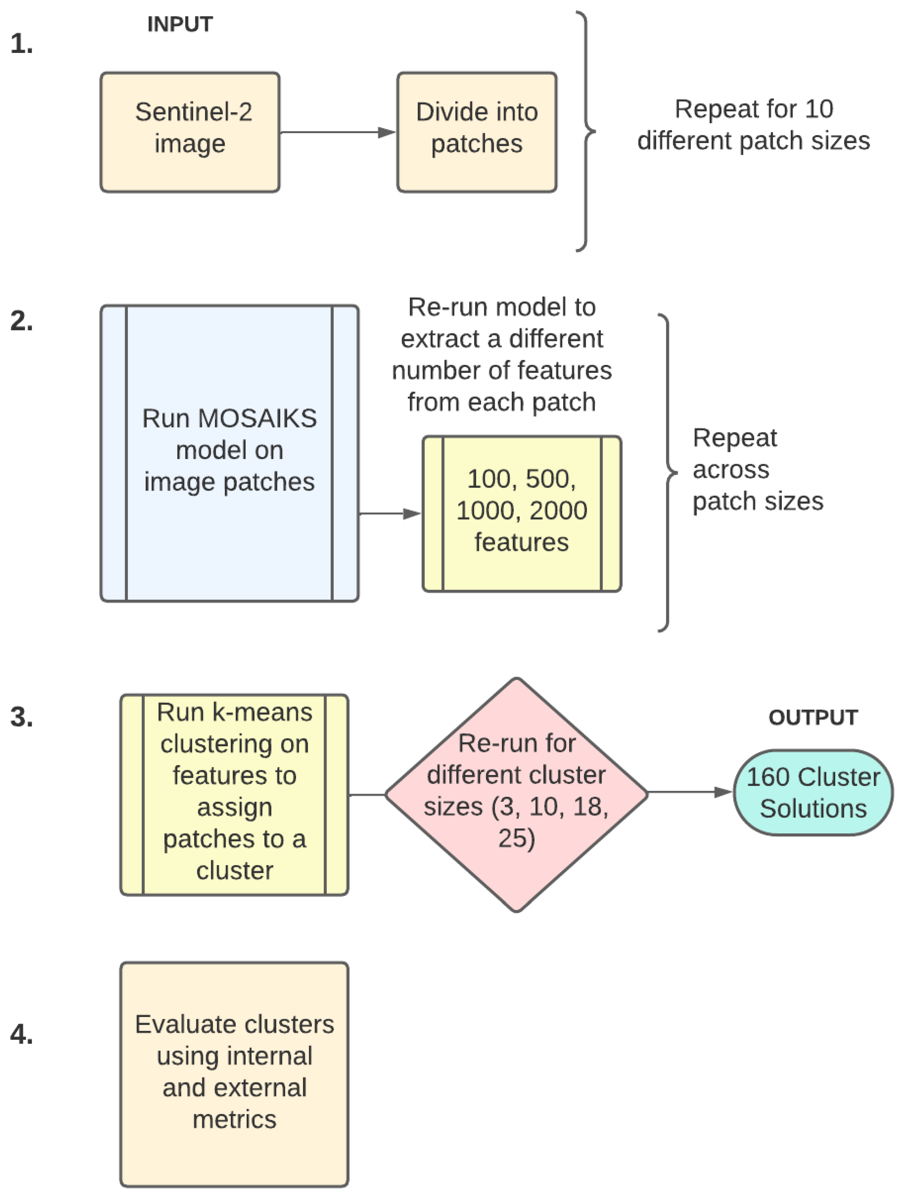
The following paper tests whether features extracted from satellite imagery using unsupervised machine learning can be used as the only input to a clustering algorithm to identify housing submarkets. We use the feature extraction method proposed by Rolf et al. [38] which is general purpose, accessible, and has a relatively low computational cost. Sub-market clusters are created at various geographic scales by altering the size of the satellite image patches in the feature extraction model from building to neighbourhood and regional intra-urban scales. We validate how well the clusters represent sub-markets using housing listings data to analyse the homogeneity of housing prices and attributes within the clusters. We also experiment with the number of features in the model and the number of resulting clusters.

2. Materials and Methods

2.1. Satellite Imagery

The main source of data employed in the study is high-resolution multispectral satellite imagery of the earth’s surface, sourced from the European Space Agency (ESA) Sentinel mission. Sentinel 2 provides global coverage of the earth’s surface every 10 days; its high spatial and temporal resolution is a key advantage of the data compared to many traditional sources. The data are openly available at three spatial resolutions, 10 m, 20 m, and 60 m per pixel, and we employ the satellite imagery with the highest resolution (10 m per pixel) to capture the most detail possible. We take the satellite imagery for the city of Madrid (604.3 km²), a densely populated urban area, with a population of around 3.2 million people. The housing market is characterised by high heterogeneity in housing prices and segregation between neighbourhoods [39], making it an interesting case study.

We searched the data using the Spatio-Temporal Assett Catalog (STAC) and the ‘pystac_client’ (0.7.6) python package, within the Microsoft Planetary Computer Hub {2023-01-26} [40]. The Microsoft Planetary Data Catalogue holds many collections of remote sensing and spatiotemporal data. Accessing the data through the catalogue, which is stored on the cloud, is much more computationally efficient than downloading the data locally. We searched the Sentinel 2 catalogue using the geographic boundary of Madrid city to find the STAC item that intersects with our study area. One STAC item, a GeoJSON object, covers Madrid city. We also searched over time, from 2017 and 2019, to find the STAC item with the lowest cloud cover, using the ‘eo’ (1.1.0) extension. We identified the item taken on the 13 February 2019 as the least cloudy. Searching the imagery across space and time is very efficient using this approach. Figure 1 shows Madrid’s city boundary and the data (Sentinel 2 Level-2A image) for the study.

In order to format the satellite image for the feature extraction model, the image must be split into smaller squares, also called patches or tiles. We tested ten different patch sizes, increasing the size (length and width) of the image patches by 20 pixels in the first instance and then 40 pixels each time (

Table 1. Description of the satellite image patches used at each scale.

Scale	Number of Patches	Patch Size (Pixels)	Area of a Patch (km2)
1	12,688	30 × 30	90
2	4526	50 × 50	250
3	1360	90 × 90	810
4	672	130 × 130	1690
5	378	170 × 170	2890
6	238	210 × 210	4410
7	168	250 × 250	6250
8	120	290 × 290	8410
9	99	330 × 330	10,890
10	72	370 × 370	13,690

). To vary the size of the satellite image patches, we constructed ten geometric grids over Madrid City using a projected coordinate reference system. Each grid is a geodataframe with a different size of grid cells; for example, Figure 1 shows the grid with the largest cells. Madrid is split into 72 patches with a full patch covering 13,690 km². Figure 2a shows the smallest patch, covering 90 km², Figure 2b shows a medium size patch covering 1690 km², and finally Figure 2c shows a larger patch of 10,890 km².

The final stage of image pre-processing involves converting the pixel values of each image patch into a Pytorch tensor, a multi-dimensional array. Each resulting image tensor has three dimensions: height, width (patch length in pixels), and number of channels (Red, Green, Blue). We used three channels, as this is the structure required for the feature extraction model. We then normalised the pixel values, scaling them from zero to one; this is also a requirement for the model. These values are stored in a matrix and form the input for the model.

2.2. Housing Listings Data

The second key source of data for the study is from Idealista, a major real estate listings portal in Southern Europe. Online real estate platforms are used to rent, buy, and sell properties. Homeowners or agents advertise properties for sale, and include information on structural attributes of the property and the asking price. We employ individual level, geographically referenced data about the property market created through this service to measure the homogeneity of the housing sub-markets across patch sizes.

The data are openly available from Idealista for Madrid, Valencia, and Barcelona (2018), and it can be accessed in reference [41]. The data include 94,814 listings posted on Idealista for the city of Madrid; we exclude 19,011 listings which remain in the portal over 4 months and are repeated in the dataset, leaving 75,803 properties. We keep the last repeated listing, as this is best representative of the final price. The variables we employ are shown in

Table 2. Descriptive statistics on housing attribute variables from Idealista.

Variable	Mean	Std. Dev.	Min.	Max.	Moran’s I
Price (EUR)	389,264	412,792	21,000	8,133,000	0.60
Area (m2)	100.25	66.44	21	985	0.43
Construction Year	1965	28.92	1623	2018	0.56

. Idealista retrieves the construction year and age of the property from the Cadastral, the official building register in Spain.

The average house in Madrid (2018) is EUR 389,264, has an area of 100.25 m², and was built in 1965 (Table 2). However, the std. deviation indicates the property characteristics deviate substantially from the average (Table 2). Furthermore, the characteristics show considerable positive spatial autocorrelation, and geographically proximate properties tend to exhibit similar characteristics, as indicated by Moran’s I values above 0.4. The housing price shows the strongest autocorrelation (0.6), which supports the existence of a systematic spatial pattern and spatial clustering in housing values. It is therefore suitable to aggregate the properties into spatial units.

2.3. Feature Extraction Model

We utilise the first stage of the machine learning model MOSAIKS (Multi-task Observation using Satellite Imagery & Kitchen Sinks) [38] to translate the essential information in the satellite image patches into vector representations. The ‘featurisation’ is unsupervised and uses representation learning, meaning the model can automatically discover meaningful patterns in big and complex raw data, such as images or text, without labelled inputs. For images, the model condenses the image texture, colour, and spatial structure into essential ‘features’. The same set of ‘features’ extracted using the MOSAIKS model can then be used to predict a range of outcomes (e.g., population density, weather, housing prices, and biodiversity) because the feature vector contains all the essential patterns in the image, rather than specific labelled features. The number of ‘features’ extracted from the imagery is specified in the model parameters; according to the original paper extracting 100 features explains a substantial amount of variation in the outcome variables. To test the sensitivity of the model to the number of features, we also experiment with using 500, 1000, and 2000 features.

The MOSAIKS model is based on the technique Random Kitchen Sinks, a machine learning algorithm which searches for an array of features in data at random. Its name comes from the phrase ‘everything but the kitchen sink’, which means a much larger number of things than is necessary. The MOSAIKS featurisation encapsulates this idea, as it condenses all the information in the satellite image based on the premise that some of this information will be relevant to any outcome variable.

Random Kitchen Sinks are adapted to satellite data to extract Random Convolutional Features (RCF) from input imagery. RCF works by choosing a random sample of image patches and convolving these patches across the entire satellite image [42], a process referred to as average-pooling. A non-linear activation function called Rectified Linear Unit (ReLU) is then applied to the convolved patches, generating an activation map for each patch [43]. Subsequently, the model employs adaptive average pooling over the image pixels to condense the dimensions of the activation maps to a singular value, effectively representing the intensity of a ‘feature’ within the image. The approach assumes that most information is represented in local-level image structure. We test this assumption, and apply the model to detect features with a larger spatial structure by using larger patches (Table 1).

The ‘features’ extracted from MOSAIKS have been shown to have a similar predictive accuracy to CNNs. The approach, however, is much less computationally intense, since it does not require training to optimise the weights. Instead, the weights for MOSAIKS are randomly initialised by drawing from random patches in the sample. We choose the MOSAIKS method for the study primarily because it can be deployed on a standard laptop without the need for a Graphics Processing Unit (GPU). Since the objective of the study is to experiment with scale, we also needed to be able to easily re-run the model using numerous patch sizes. The MOSAIKS method was able to simplify and reduce the computational cost of this process. Furthermore, since housing sub-markets are influenced by a range of known and unknown structural and locational variables, we see MOSAIKS as a suitable approach to capture all the information contained in the image.

Patches with a length and height of three pixels were found to perform best in the estimation of housing prices in the original MOSAIKS paper [38]. We experimented with larger patch sizes to detect features with a larger spatial structure (Table 1). We contribute to a more nuanced understanding of how the MOSAIKS model performs with different patch sizes, also referred to as scales. In addition, we apply the MOSAIKS model to imagery at the local city level rather than the country level, as in the original application [38].

2.4. K-Means Clustering

The next stage of analysis uses the feature vectors as an input to a clustering algorithm to cluster image patches with similar features into groups. Clustering is an unsupervised type of statistical learning, meaning the patches are organized into groups based on the ‘features’, but the groups are not known beforehand; rather, we aim to discover these groups or clusters from the image ‘features’ themselves. Each group is known as a cluster, and observations within a cluster are more similar to each other than to those in different clusters.

We use a K-means clustering algorithm. K-means randomly assigns each observation in the dataset to a cluster; the mean of the covariates is then calculated for each cluster. Each observation is then reassigned to the cluster with the closest mean, iterating through the assignment of data points to clusters until no more reassignments are necessary [44]. This iterative process continues until the variance within clusters cannot be further minimized, quantified by the summed distance of all points to their respective centroids. An essential pre-processing step involves scaling the feature embeddings, ensuring that larger-sized features do not disproportionately influence the clustering process [38]. K-means is chosen as it is computationally efficient and works to minimise the within cluster variance on the features, which is the objective when identifying housing submarkets. One consideration for K-means is that the number of clusters must be pre-specified. In our implementation, we test four different cluster sizes (3, 10, 18, 25). There is no pre-defined or known number of existing housing sub-markets or clusters, so we test up to 25 clusters.

Clustering is a commonly used method in geographic data science to discover underlying structural and spatial patterns within multi-dimensional or multi-variate data. K-means allows us summarise the multitude of ‘features’ extracted from the imagery into a label for each image patch. Patches with the same label have similar ‘features’. We then assign the housing points described in Section 2.2 a label, according to its geographically referenced image patch. We are then able to visualise the spatial patterns of the cluster groups associated with a residential building. We run the clustering separately for each scale, assigning the properties a group based on the features from ten different image patch sizes. At each scale, we also repeat the clustering for four different cluster sizes.

2.5. Assessment of the Clusters

The final stage of the analysis involves the assessment of the homogeneity and quality of the clusters across scales and cluster sizes. First, we employ three internal validations which are commonly used to evaluate the performance of the k-means clustering. The silhouette score is a measure that evaluates how well-defined clusters are, by examining both intra-cluster cohesion and inter-cluster separation [45]. The score is calculated by measuring the mean distance of all points within a cluster to the cluster centroid, contrasting it with the distance to the centroids of other clusters. The silhouette score is particularly valuable for handling high-dimensional datasets, as it ranges from −1 (indicating poorly defined clusters) to 1 (indicating well-defined clusters). However, the score is sensitive to cluster size, so we compare across clusters with the same size using the silhouette score.

The Davies–Bouldin (DB) Index offers a means of evaluating cluster compactness by averaging the similarity ratios for each cluster, defined as the average distance from a point in the cluster to the points in its most similar cluster, excluding its own [44]. The final index is derived by averaging these similarity ratios across all clusters. A lower Davies–Bouldin index value is desirable, as it signifies well-separated and compact clusters [46]. Unlike the silhouette score, it makes no assumptions about the shape of the clusters, so we use it to compare across models of different cluster sizes.

The Calinski–Harabasz score gives an idea of the compactness of clusters, calculated as a ratio of within cluster dispersion and between cluster dispersion [47]. It measures how similar an observation is to its own cluster compared to other clusters, making it useful to understand how well-defined clusters are. Based on the idea that well-defined clusters have a large between-cluster variance and a small within-cluster variance, a higher Calinski–Harabasz indicates better-defined clusters [48]. The measure is useful as it does not require any labels and is less sensitive to the size of the clusters and dataset.

Secondly, we calculate three ‘external’ evaluation metrics using the housing listings data. A key objective of the research is to examine which scale(s) or patch sizes result in the most homogenous housing clusters. As such, we measure the homogeneity of properties within the clusters. For each cluster solution (across patch size and cluster size), we calculate the average within cluster std. deviation in key housing attributes (Price, Size, and Age, Table 2). The standard deviation measures the amount of dispersion of the data relative to their mean. For example, we calculate the difference between each property’s price and the average price for its cluster. We sum this difference for each cluster to get the intra-cluster std. deviation in price. We sum the variation for each cluster and divide by the number of clusters to get the average within cluster variation. We do this so the measure is comparable across solutions with different cluster sizes.

The external analysis is instrumental in understanding the compactness and separability of the derived clusters or sub-markets in terms of their housing attributes across the hyperparameters (cluster and patch size). The hyperparameter values which result in the lowest within-cluster variation in housing attributes, particularly the housing price, is how we assess the best fit model(s) in line with the theory of housing sub-markets.

2.6. Regression Analysis

To further test effect of the model parameters (scale, number of clusters, and number of features) on the internal and external evaluation metrics and test whether this effect is significant, we use an Ordinary Least Squares (OLS) regression model (Equation (1)), and then the same model with quadratic terms (Equation (2)).

Y = β₀ + β₁X₁ + β₂X₂ + β₃X₃ + ε

(1)

Y = β₀ + β₁X₁ + β₂X₂ + β₃X₃ + β₄X₁² + β₅X₂² + β₆X₃² + ε

(2)

Each observation in the dataset is a clustering solution calculated with a different patch size, number of clusters, and number of extracted features. We regress the hyperparameters, the dependent variables, against the evaluation metrics (internal and external). We then run another regression model, this time also including the square of the independent variables as predictors in the models (β₄X₁² + β₅X₂² + β₆X₃²), to capture the non-linearity between the independent and dependent variables (Equation (2)). These quadratic terms tell us about the shape of the relationship between the hyperparameters and evaluation metrics. Unlike the linear model, the change in Y now depends on the value of X. To interpret these coefficients, we select an X value, e.g., number of clusters = 14. We multiply the X value (14) by the linear coefficient. We then square the chosen X value (14²) and multiply this value by the squared coefficient of cluster size. We then sum these values to find the effect on Y for different values of X, repeating this process until we find the value(s) of X at which the slope changes.

We present the results of these two models using six outcome variables: the three internal (Silhouette Score, Davies-Bouldin Index, and the Calinski–Harabasz Score), and three external evaluation metrics (average std. deviation per cluster in housing price, age, and size). We use the significance and size of the coefficients to infer their effect on the validation measure, and are particularly interested in how the scale and cluster size impacts the clustering evaluation metric.

A summary of the entire pipeline is provided in Figure 3.

3. Results

3.1. Exploring Scale Effects on Clusters

We use scatter plots to visualise the relationship between patch size and quality of the clustering for all the cluster solutions. This allows us to identify if there are trends in the performance of the clustering across the patch size. We first assess the clustering solutions using the internal validation metrics. Figure 4 shows the silhouette scores for clusters across patch sizes; a higher score indicates higher within-cluster cohesion. The score cannot be compared across models with different cluster sizes.

Overall, the silhouette scores are above zero, indicating relatively distinct clusters for all models. We observe that the relationship between scale and the silhouette score is dependent on the number of clusters. For three clusters, smaller patches (30 × 30, 50 × 50 and 90 × 90) tend to result in slightly more distinct clusters. However, we see 330 × 330 pixel patches as resulting in the most cohesive clusters, particularly using 100 features (silhouette score = 0.45), indicating three cohesive clusters or submarkets at the widest spatial scale. For identifying ten clusters from the image features, the relationship between patch size and silhouette score seems positive from 250 × 250 pixels: as the patch size increases, so does the silhouette score. Using patch sizes above 250 × 250 pixels results in the most cohesive sub-markets or clusters. Again, using fewer features seems to create more cohesive groups in the data. For 18 clusters, the findings are similar, with 330 × 330 pixel patch sizes and 100 features resulting in the highest score (0.25). For identifying a larger number of clusters (25), we see that small and large patch sizes have higher silhouette scores of more than 0.2. However the patch size that results in the most cohesive clusters is clearly 250 × 250 pixels. Overall, embedding fewer features (100) from the imagery results in higher silhouette scores, which is also more computationally efficient.

The Davies–Bouldin index is the next measure we used to understand scale effects on the clusters. A lower Davies–Bouldin index indicates better clustering. For identifying three clusters we find the optimal Davies–Bouldin scores for patches of 30 × 30 to 100 × 100 pixels. The index increases with patch size until 300 × 300 pixels, at which point we observe a drop in the score to 1.12. Again, we find that extracting 100 features results in more cohesive clusters.

Similar to the patterns observed for the silhouette score, we observe a change in the direction of the relationship with patch size and Davies–Bouldin index for larger cluster sizes. For 10 or more clusters, the relationship is negative; as the patches get bigger, the Davies–Bouldin index gets smaller indicating a better cluster solution with more separate clusters (Figure 5). We find the lowest score (around 0.8) for the largest patches (360 × 360) and cluster sizes (18 and 25). Overall, this suggests that for identifying more, well-separated clusters larger patches (360 × 360 pixels) are better.

Finally, Figure 6 shows the Calinski–Harabasz score using a cluster size of 18. We choose to present one cluster size as the trend between scale and Calinski–Harabasz score was identical for the other cluster sizes (three, ten, and twenty-five), a slightly different story to the trends presented in Figure 4 and Figure 5. A larger Calinski–Harabasz score indicates that clusters have lower within-cluster variability and larger between-cluster variability, indicating a better clustering solution. The Calinski–Harabasz score is higher for the smallest patch sizes. The score starts to increase from a patch size of 130 × 130 pixels. The Calinski–Harabasz score suggests more compact and internally cohesive clusters for smaller patch sizes for every cluster size presented. Again, using 100 features results in optimal scores.

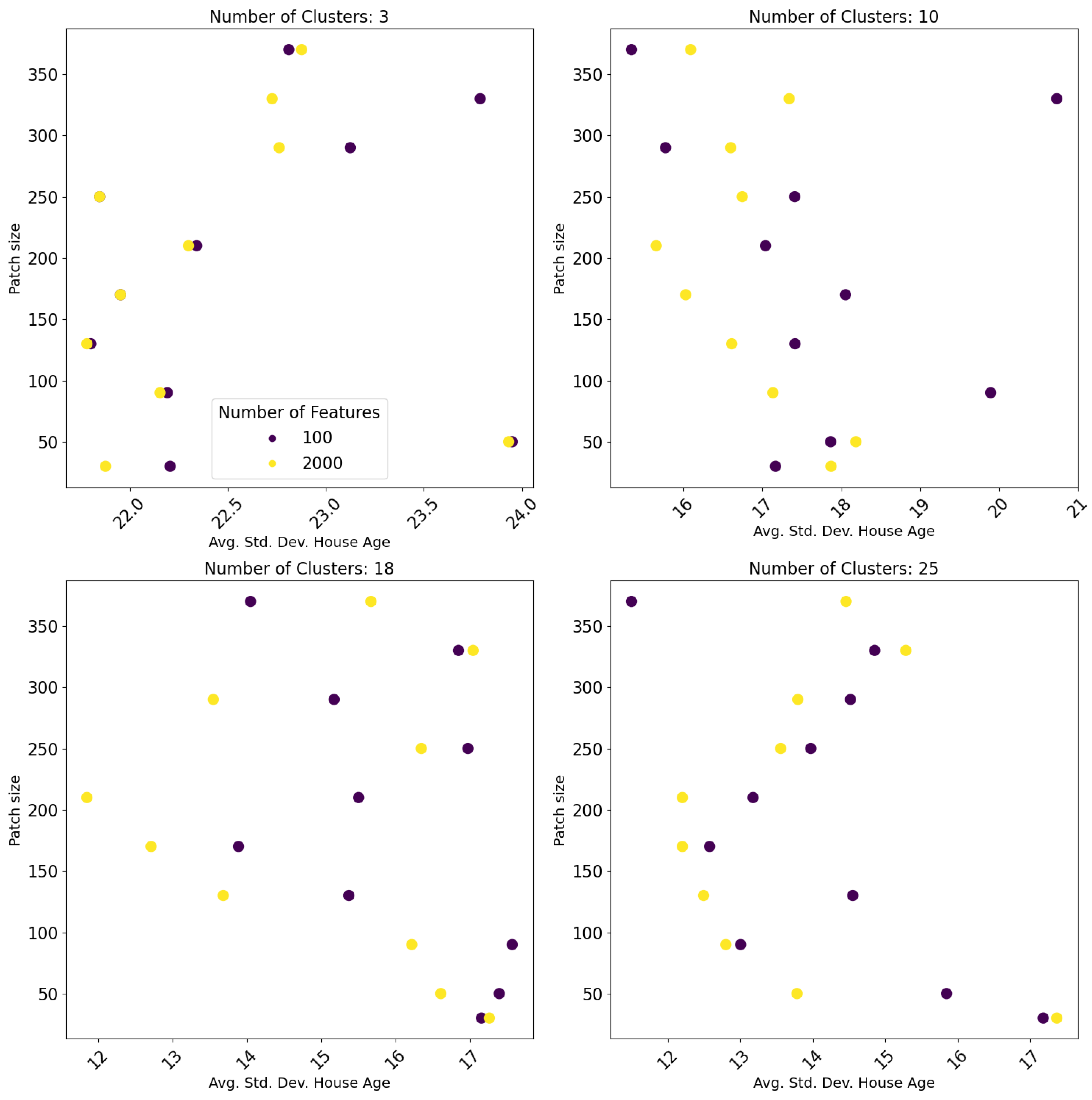
After we assessed the cluster solutions using internal measures, we validated them using ground-truth data on housing prices and attributes (Table 2). The house price is the most common characteristic used to define housing sub-markets [10]. We are looking for the clustering solution and patch size that minimises the within-cluster variation in housing prices, in line with the theory of housing sub-markets. Interestingly, we observe slightly different trends to those found using the internal measures. The external measures are arguably better for assessing how well we identified housing sub-markets from the features.

For a cluster size of three, ten and eighteen, we observe the smallest mean std. deviation in housing prices within clusters using a patch size of 200 × 200–250 × 250 pixels (Figure 7). Overall, we observe the highest within-cluster variation in housing price for the smallest patch sizes. The variation within clusters decreases as the patches get bigger, until 250 × 250 pixels, from which point the variation starts to increase again. This suggests that the smaller scales may not be suitable for identifying three homogenous housing sub-markets.

Overall, as the cluster size increases the variation in prices per cluster decreases, suggesting that 25 + clusters or sub-markets exist in the features. For identifying 25 clusters, the trend with housing price homogeneity and patch size becomes less clear cut. For models using 2000 features and smaller patch sizes (50 × 50–200 × 200) the variation in housing prices within clusters is lower than for the larger patches, with the exception of the smallest (30 × 30 pixels) and largest (360 × 360) patch. Unlike the findings using the internal outcome measures, Figure 7 shows that generally, extracting more features (2000) from each patch results in more homogenous housing price clusters than fewer features (100), particularly for defining more than 3 clusters. Suggesting that extracting more features from the imagery optimises the identification of housing submarkets and facilitates better differentiation between the housing sub-markets at a more granular level.

Overall, the relationship between patch size and house price variation seems to be non-linear and dependent on the number of clusters. Although across all cluster sizes a patch size of around 200 × 200 seems to result in an optimal house price variation per cluster. The optimisation of sub-markets at varied geographic scales seems to reflect the spatial-hierarchical structure of housing sub-markets, and the existence of sub-markets at several spatial scales. We find very similar trends for the area and construction year variables (Figure A1 and Figure A2).

3.2. Regression Analysis

We further assessed the relationship between scale, number of features, and number of clusters, and the internal and external validation metrics, using a regression model. Holding other variables constant, a one pixel increase in patch size results in a decrease in the average within-cluster std. deviation in housing price of EUR 98.28 (

Table 3. Baseline OLS regression coefficients.

X Variable	Price (EUR)	Area (m2)	Construction Year	Silhouette Score	Calinski–Harabasz	Davies–Bouldin
Scale	−98.28 ***	−0.006	−0.001	8.922 × 10−5 ***	−5.99 ***	−0.0011 ***
Num. of Clusters	−5090.23 ***	−0.80 ***	−0.37 ***	−0.0062 ***	−30.44 ***	−0.0059 ***
Num. of Features	−6.32 ***	−0.001 ***	−0.0002	−1.106 × 10−5 ***	−0.007	5.639 × 10−5 ***
R-Squared	0.71	0.61	0.77	0.76	0.40	0.55

*** p < 0.01.

). According to these results, larger patches are therefore optimal for minimising the within-cluster house price variation, indicating the importance of features at a wider spatial scale for housing sub-markets. Increasing the number of clusters also has a significant, relatively large, negative effect on the variation in housing prices (−EUR 5090.23 ***), suggesting that more clusters are beneficial for capturing homogenous market segments in terms of housing price. Holding other variables constant, increasing the number of features by one decreases the average within-cluster variation in housing prices slightly (−EUR 6.32 ***), meaning more features are preferred. However, the decrease in price variance is relatively small.

The scale does not have a significant impact on the average variation in housing age and size within clusters. These housing attributes are therefore less significant indicators of sub-markets across scales. However, increasing the number of clusters does have a significant and negative effect on average within-cluster variation in property area (−0.80 ***) and age (−0.37 ***), although this effect is fairly small. Again, this supports the identification of more clusters for capturing differences in housing attributes between submarkets.

According to the internal validation measures, scale has a significant impact on the quality of the identified clusters. Increasing the patch size by one-pixel results in a small increase in the silhouette score, indicating marginally better-defined clusters (8.922 × 10⁻⁵ ***). The Davies–Bouldin index also shows a small, significant decrease (−0.0011 ***) as the patch size increases, as a lower score is preferable; larger patches also result in better quality clustering according to this measure. In contrast, the Calinski–Harabasz score shows a decrease when patch size increases by one pixel (−5.99 ***), indicating that smaller patches are optimal. Increasing the number of clusters also has a negative effect on the Calinski–Harabasz score (−30.44 ***), which supports a preference for fewer clusters. The trends identified from this score oppose what we find for the other validation metrics.

We implement the regression model again including the squared terms of the predictor variables, since some of the relationships between outcome and predictors exhibited non-linearity in the scatterplots. Generally, we see an increase in the R² for the quadratic models, signalling a better model fit when accounting for non-linearity in the relationship with the hyper parameters and external outcome variables (

Table 4. Linear-Quadratic regression model results.

Variable	Price (EUR)	Area (m2)	Construction Year	Silhouette Score	Calinski–Harabasz	Davies–Bouldin
Scale	−340.25 ***	−0.03 **	−0.022 ***	−5.572 × 10−5	−25.38 ***	−0.0003
Scale2	0.61 ***	7.145 × 10−5 **	5.22 × 10−5 ***	3.699 × 10−7 **	0.049 ***	−2.107 × 10−6 **
Num. of Clusters	−5090.23 ***	−0.80 ***	−0.37 ***	−0.0062 ***	−30.44 ***	−0.0059 ***
Num. of Clusters2	284.84 ***	−0.0449 ***	0.019 ***	0.0004 ***	2.10 **	0.000006
Num. of Features	−21.05 **	−0.0038	−0.0013 **	−4.245 × 10−5 ***	−0.12	0.0002 ***
Num. of Features2	0.006	1.254 × 10−6	5.035 × 10−7 **	1.443 × 10−8 ***	5.194 × 10−5	−7.196 × 10−8 ***
R-Squared	0.81	0.70	0.89	0.87	0.62	0.58

** p < 0.05; *** p < 0.01.

). We use the quadratic terms to understand the size and slope of the relationship between the scale, number of clusters and number of features and the validation scores.

Using variation in housing price as the outcome variable, the scale and cluster size coefficients are significant. For the average scale (patch size of 192 × 192 pixels), the change in within-cluster house price variation with a one pixel increase in the patch size is negative (−EUR 42,840.96). In contrast, for a smaller patch size of 30 × 30 pixels, the decrease in average within-cluster house price variation for a one pixel increase in patch size is much smaller (−EUR 9658.50). This suggests that, as the patches get bigger, the negative effect on within-cluster house price variation also gets stronger, supporting the inclusion of larger patches and wider spatial structures for estimating homogenous hosing submarkets.

In terms of the number of clusters, we find a positive effect for the squared (quadratic) term against within-cluster housing variation. For the average number of clusters (14), increasing the number of clusters by one results in a decrease in average within-cluster house price variation of −EUR 15,434. We find the largest decrease in within-cluster house price variation by adding one cluster for cluster sizes 8–14. For more than 15 clusters, the amount of house-price variation within the clusters increases the addition of another cluster, meaning that the clusters are less homogenous in housing price, supporting the identification of between 8 and 14 housing-price sub-markets in the features.

Using the average variation in housing size or area as the outcome variable, we find that number of clusters is the only significant explanatory variable. For the average of 14 clusters increasing the number of clusters by one results in a decrease in the average within-cluster variation in housing size (−20 m²). From 16 clusters this decrease in within-cluster variation becomes smaller (−11 m²), suggesting adding more clusters from this point has a weaker effect on average within-cluster homogeneity, although the clusters still become more homogenous in housing size.

For housing age (construction year), the linear number of clusters and the scale coefficients are significant and negative, although small (−0.37 *** and −0.022 *** respectively). Increasing the number of clusters by 1 from the average of 14 results in a decrease in the average within-cluster variation in construction year (−1.5 years). This is the largest decrease in construction-year variation across the range of cluster sizes. The results indicate that for different housing characteristics, a different number of sub-markets is optimal, supporting the hierarchical nature of housing sub-markets and attributes. The significance of scale for housing-price variation within clusters supports the consideration of this variable as a key indicator of hierarchical housing sub-markets.

We find generally slightly higher R² values for the external housing outcome models and the Silhouette score, than for the Calinski-Harabasz score and Davies-Bouldin index. This suggests that the housing data and Silhouette score are optimal to validate how the clusters are affected by the scale, size of the sub-markets and the number of features, as the hyperparameters explain more of the variation in these metrics. As well, it suggests that there are parameters which impact the internal validation score across scales other than the ones we considered.

3.3. Mapping the Clusters

The cluster groups identified represent similar groups of housing based on the information contained in the satellite image. We now present maps of two solutions in order to illustrate the impact of patch size on the resulting clusters, show the spatial patterns to the clusters, and therefore show the potential of the method for the delineation of spatial housing segments. Figure 8 maps the clusters for the smallest patch size we experimented with.

There are some interesting patterns to the spatial distribution of the clusters, with strong clustering over space. We can see that cluster A is found in the centre of Madrid, and this sub-market is densely populated with residential buildings. Bordering cluster A is cluster B, the second largest housing sub-market which appears in central outer suburbs, where we also see a lower density of points than in the very centre. In the outer neighbourhoods of Madrid, we find that housing sub-markets are less dense and more fragmented in cluster group. We see cluster C located north and south of the outskirts of the city centre in Madrid. The cluster patterns seem to show some similarities and slight differences compared to the regional administrative boundaries.

Figure 9 shows a clustering solution using the largest patch size (370 × 370 pixels). Larger patches were shown as preferable for capturing homogeneity within clusters in external housing characteristics, and around 10 clusters were shown as optimal for minimising the average within-cluster variation in housing prices in the regression model. We see a clear north–south divide around the city centre, with different cluster labels in different regions of the city. We see the majority of the north of the city centre is cluster A, whereas cluster B is prominent in the south of Madrid. In the outer neighbourhoods, on the edge of the city, we commonly find cluster C. We also find cluster D located in the southern outer suburbs. Figure 9 shows a clear spatial pattern and autocorrelation to the clusters, which are based on features of the built environment extracted from satellite imagery. The maps suggest there are strong spatial differences in the features of the built environment and therefore sub-markets. In comparison to Figure 8, we see that using larger patch sizes means we lose some definition and spatial granularity in the clustering. However, we find similar total within-cluster house price variation for both maps, showing how sub-markets form at local and global intra-urban scales.

4. Discussion

This study used features extracted from aerial imagery to segment housing sub-markets. We assess how well the clustering performs across patch and cluster size in line with the definition of a housing sub-market as ‘a geographic area where the price of housing service is constant’ [14].

We found that the approach proved useful for identifying the scale at which the housing sub-markets exist, and the number sub-markets or clusters the unitary market should be divided into. These two factors were shown to be intrinsically linked, with the optimal scale depending on the number of clusters. For more clusters, smaller patch sizes became useful for minimising within-cluster variation in housing prices. Evidence has shown that differences exist in hedonic house prices at the intra-urban scale [39]. These results have highlighted the effect of scale on the homogeneity of the identified housing sub-markets, and there is no one ‘optimal’ scale, rather different scales can be optimised to capture different sub-markets and housing attributes.

We find a non-linear relationship between patch size and house price homogeneity. For identifying 25 clusters within Madrid, using the smallest and largest patch sizes resulted in lowest house price variation within the clusters. Using medium patch sizes (210 × 210 pixels) resulted in the lowest within-cluster variability for housing size and area (Appendix A and Appendix B) for 18 clusters. For larger cluster sizes, smaller patches were also optimal. This also supports the hierarchical nature of housing sub-markets and existence of sub-markets at various intra-urban scales [8]. Although, according to the regression analysis the clusters are more homogenous in price with larger patches, and this relationship gets stronger as the patch size increases.

The results indicate the existence of strong regional intra-urban housing sub-markets and the importance of the wider neighbourhood for local house prices. This is an important contribution of the research to the discussion on how much of the neighbourhood is relevant in the estimation of house prices [32,49]. The results support the finding that a larger neighbourhood context is important for house prices, in line with some previous research [35]. The results also show that, contrary to previous conclusions [38], larger patch sizes which capture wider image structure can be better for studying housing prices, particularly at the city level.

It is possible that the resolution of the imagery meant that smaller patch sizes were unable to capture the texture of the image. Figure 2 shows some slight blurriness to the smallest patch sizes. Using higher-resolution imagery for identifying housing sub-markets at the fine grain intra-urban scale would be a key area of further research. This data, however, are larger in size, limiting the ease of implementing the analysis.

The results supported the spatial approach to the identification of housing sub-markets, due to the spatial patterns of the clusters shown in Figure 8 and Figure 9. Whether sub-markets are spatial or a-spatial has been debated in the literature [20]. The k-means clustering algorithm does not have any spatial parameters, but the clusters show spatial autocorrelation in the maps presented, and similar clusters are found nearby one another, indicating that the information in the image shows key spatial differences. Housing clusters on the periphery of the city appear to be more fragmented than in the central areas, where sub-markets are more spatially homogenous.

The quality of the identified clusters depends on the outcome measure used, and we considered both internal and external validation measures. The internal measures showed varied preferences for the optimal scale. The Davies–Bouldin index and the Silhouette score showed a preference for larger scales (Table 3). In contrast, for the Calinski–Harabasz score, smaller scales resulted in better scores. Whilst these scores are useful for assessing the quality of the clusters, they do not consider their relation to housing sub-markets. We therefore conclude that to use this method to identify housing sub-markets, external validation measures and housing data are required.

The method has great potential to dynamically identify sub-markets according to different housing attributes. This is advantageous since housing sub-markets can be defined on a vast array of attributes and many features have been suggested in the literature as important, including price, location, structural property and neighbourhood attributes [21]. Below the metropolitan level, sub-markets can be delineated by socio-economic characteristics such as race or income levels, and the spatial configuration of these variables also varies by scale [24]. Multiple geographic units, from the immediate neighbourhood to the city level, interact to influence house prices [4]. This creates a complex system where understanding one level is not enough to fully explain the price variation. The method is useful for understanding how different variables correlate over scale and cluster size, which is difficult when using aggregated data at one spatial scale.

The method could be used to identify housing submarkets across multiple scales, which has been shown as an effective approach in recent multi-level modelling frameworks [50]. The benefit of being able to scale the housing sub-markets up and down can help to overcome the effect of the ecological fallacy, where a pattern at one scale may be not be reflected at another. Using different patch sizes facilitates this, although it would be unfeasible to test every possible patch size using this approach. The selection of which patch sizes to test is in some way arbitrary and depends on the user’s choice. It would be necessary to also try larger cluster sizes. One limitation of the approach is the patches must be a uniform square shape with equal height and width. In reality the sub-markets may not meet this expectation and form irregular shapes over space.

Further research could conduct the analysis over time to identify changes to the city’s housing market from satellite imagery, for example to detect changes to the spatial pattern of the clusters. The drivers of spatial change in urban housing submarkets is under-researched. It would be interesting to explore whether sub-market changes can be seen in changes to the built environment; new developments have been shown as associated with sub-market change [17]. The relationship between scale and housing submarkets may also have a key temporal dimension, which this study did not consider. In addition, further exploration is required to understand which ‘features’ are important in the delineation of clusters, which could be done using a machine learning regression approach.

5. Conclusions

This study demonstrates the usefulness of satellite imagery to measure the homogeneity of housing sub-markets across scales, using an example from the urban landscape of Madrid. The MOSAIKS featurisation method is suited to this task since the size of the image patches inputted into the model can efficiently be changed. Extracting features from Sentinel 2 satellite imagery in this way facilitates classification of properties into housing submarkets across multiple scales, which is usually difficult due to the already aggregated nature of housing data.

Scale was shown to significantly impact homogeneity within clusters, with larger scales leading to more homogenous sub-markets in terms of price and construction year. The accessibility of the method and ease of accessing the data is a key benefit of the study; the analysis can be undertaken without the need for a GPU and the location of analysis can easily be changed in the pipeline. The approach could provide a standardised way to identify sub-markets across cities and countries, and be useful for non-specialist users such as governments and policy-makers. Additionally, there is great potential for satellite imagery to be used to identify sub-market change over time due to its high temporal frequency.

Furthermore, the features may be capturing attributes of the built environment which are difficult to measure, a key benefit of extracting all the information from the image in an unsupervised manor. However, more research is needed to test this hypothesis. Additionally, some form of external housing data is required to validate the cluster homogeneity. Applicability in contexts lacking housing listings data requires further exploration, although data-poor contexts are where this method could be really useful to identify spatial housing market segments.

One challenge encountered during the study was the application of the MOSAIKS method to other satellite image data. It proved difficult to run the analysis with satellite imagery downloaded locally, due to the size of the data. Since the Sentinel 2 image data can be accessed through a cloud based data catalogue, the analysis was fairly easy to implement with the same pipeline and imagery as in MOSAIKS. There were not many technical challenges adjusting their pipeline. However, it would be necessary to repeat the study with more granular imagery to understand whether the poor performance of smaller patch sizes was related the image resolution. Moreover, identifying the point at which having higher resolution imagery does not improve the featurisation step would be useful for the future of using satellite imagery for this kind of urban analysis.