Article

Exploring Switzerland’s Land Cover Change Dynamics Using a National Statistical Survey

by
Isabel Nicholson Thomas
1 and
Gregory Giuliani
1,2,*
1
EnviroSPACE Laboratory, Institute for Environmental Sciences, University of Geneva, Bd. Carl-Vogt 66, 1205 Geneva, Switzerland
2
GRID-Geneva, Institute for Environmental Sciences, University of Geneva, Bd. Carl-Vogt 66, 1205 Geneva, Switzerland
*
Author to whom correspondence should be addressed.
Land 2023, 12(7), 1386; https://doi.org/10.3390/land12071386
Submission received: 7 June 2023 / Revised: 9 July 2023 / Accepted: 10 July 2023 / Published: 11 July 2023

Abstract

:
Timely and reliable Land Use and Cover change information is crucial to efficiently mitigate the negative impact of environmental changes. Switzerland has the ambitious objective of being a sustainable country while remaining an attractive business location with a high level of well-being. However, this aspiration is hampered by increasing pressures that are significantly impacting the environment and putting serious demands on land. In the present study, we used the national Land Cover (LC) dataset, named ArealStatistik, produced by the Federal Statistical Office, to explore the spatiotemporal patterns of Land Cover in Switzerland, providing a comprehensive assessment of land cover change at the national scale. Results indicate that, in general, Switzerland has undergone small, spatially dispersed, dynamic, and gradual change trends, with high rates of transition between low growing Brush Vegetation and forest LC classes in recent years. These pixel-level trends are more important in the lower altitude plateau and Jura regions, while greater changes in the spatial configuration of LC are observed in the alpine regions. However, findings also suggest that identifying drivers and understanding the rate of change are limited by the spatial resolution and temporal update frequency of the ArealStatistik. The ability to understand these drivers would benefit from a high-resolution annual LC dataset. Such a data product can be produced using the ArealStatistik together with dense satellite data time-series and Machine/Deep Learning techniques.

1. Introduction

The world is significantly impacted by human-induced environmental changes from local to global scales. Human well-being is critically dependent on Earth’s natural systems. Despite the agreed goal of halting land degradation, it is projected to increase in the twenty-first century under all development scenarios [1]. Consequently, land degradation is recognized as a major global environmental issue with important linkages to climate change or biodiversity loss [2]. The drivers of land degradation are predominantly local, so actions to address them should be based on the understanding of the local interplay of a range of factors.
To understand these drivers, it is crucial to apprehend how people utilize the land for socio-economic activities and to precisely map the changes of observed (bio)physical cover and use of the Earth’s surface (e.g., Land Use and Cover—LUC) [3]. Land cover (LC) is included in the list of Essential Climate Variables (ECV), on account of its relevance for assessment of changes in the climate system and its availability in the form of multiple coherent global datasets [4]. LC has been further identified as a possible Essential Biodiversity Variable [5], recognizing the potential for its detrimental impact on biodiversity of land conversion processes [6], and contributes to reporting on 14 of the 17 Sustainable Development Goals (SDGs) [7]. Moreover, LUC has been increasingly recognized as a significant actor in processes of global environmental change [8], and is both a cause and effect of climate change [9]. LUC plays a role in the sustainability of human exploitation of the natural environment, presenting a trade-off between immediate provision, and the maintenance of goods and services for future generations [10].
Therefore, LUC change can be considered a major visible indicator of the human footprint, and an essential component underpinning the development of any efficient and effective environmental and territorial policies. This includes urbanization, agricultural land loss or expansion, deforestation, afforestation, and desertification. Such LUC changes can have significant impacts on both environmental conditions (e.g., pollution, climate change) and human activities (e.g., food security, economic development). Therefore, with such a variety of forms of LUC change and consequent impacts, there is a pressing need for rigorous and systematic monitoring and analysis of LUC dynamics. They will provide evidence to stakeholders and decision-makers to promote responsible actions [11,12].
The state of LUC is highly dynamic and creates a challenge for its mapping and monitoring that remains inadequately addressed. Timely and reliable LUC change information is crucial to efficiently mitigate the negative impact of environmental changes. Traditional environmental data (e.g., field data collection) suffers from data inconsistencies caused by changes in reporting methodologies and gaps (e.g., missing measurements). The demands and expectations of users for LUC and LUC Change (LUCC) products continue to increase; consequently, accurate and up-to-date LUC and LUCC products are more important than ever, and are basic, essential inputs for policymakers [13].
Land change science (LCS) plays a pivotal role in monitoring environmental change and the sustainability of our planet’s resources. It endeavors to understand both the magnitude and spatial extent of changes in LUC over time; identify the drivers of LUC change; investigate the possible impacts and potential consequences of LUC dynamics; propose better land use planning policies; and inform relevant decision-makers. To that end, it is essential to have a comprehensive understanding of the gains and losses of LUC, including the magnitudes, locations, and timings of transitions. To quantify LUC changes across a range of scales, it is critical to have (1) a time-series of fine-resolution and temporally consistent satellite-derived LUC dataset, and (2) methods to determine LUC dynamics to identify patterns (e.g., trend, break, disturbance, degradation).
The classic approach for assessing LUC change is the use of Markovian transition matrices, in which the probability of change in a class is expressed as the ratio between the area of transition and the total area of the initial category [14,15]. As LUC are dynamic variables, changes between the largest categories should be expected even under random processes of change which do not reflect key LUC change drivers [16]. It is therefore necessary to incorporate the relative importance of the categories involved in the transition and distinguish systematic changes between LUC categories through removal of the value of expected change under random processes [17]. This Intensity Analysis has been adopted in subsequent work on assessing LUC change [18,19] and as an additional benefit, allows for the identification of important signals of change in landscapes where the dominant process may be persistent. In addition to the systematic assessment of change between and within LC classes, assessing the change in the spatial pattern of LC provides an idea of the key LUC change processes operating at the local-scale, and encapsulates the variables of fragmentation and connectivity that influence the Ecosystem Service provision [20].
Switzerland has the ambitious objective of being a sustainable country while remaining an attractive business location with a high level of well-being [21]. However, this aspiration is hampered by increasing pressures (e.g., population growth, energy demand, urbanization, high consumption of resources) that are significantly impacting the environment and putting serious demands on land [22]. The strategic importance of sustainable land management is recognized in a national (Spatial Planning Act, Spatial Strategy for Switzerland, Sustainable Development Strategy, Strategy on Biodiversity) as well as regional scale (European Green Deal), and through international policies (Sustainable Development Goals). They all agree that land can offer multiple valuable ecosystem services that are essential for human well-being [23,24] but also indicate that most ecosystems are being degraded and fragmented, and therefore not providing efficient and effective services as healthy ecosystems.
To track these changes in Switzerland, the official LUC data source is the Land Use Statistics (Arealstatistik) of the Federal Office for Statistics (FSO) obtained by visually interpreting aerial images and assigning a LC as well as a LU category of the lower-left corner of each sample point from a regular 100 m grid cell, corresponding to more than 4 million points over the country following three nomenclatures: standard (72 categories); land cover (27), and land use (46) over four-time periods (1979-85, 1992-97, 2004-09, 2013-18) [25]. Using this dataset, various studies have well documented Land Use change, such as [26,27]. Most of the national studies concentrate on Land Use change and how it can affect carbon stocks [28], species habitat [29] or urbanization and land abandonment [30]. However, less attention has been provided to Land Cover change and, currently, a comprehensive assessment of Land Cover change across all categories of the Arealstatistik at the national scale is still missing. Indeed, most research concentrates on a specific LC class, such as forest cover change [31] or cropland and grassland [32], producing information from LC data like a nationwide habitat map [33], LC degradation [34] or studying the effects on Gross Primary Production [35]
Based on these previous considerations, this study aimed to explore the spatiotemporal patterns of Land Cover change in Switzerland using the official LC data for Switzerland, therefore filling the identified gap by providing a first extensive assessment. To achieve this objective, the following questions were investigated: (1) what are the spatiotemporal patterns of major LC change in the country between 1985 and 2018; (2) what are the key LC transitions; (3) what is the intensity of change?

2. Materials and Methods

Hereafter, we present the study area, the data, and the different analytical steps to determine Land Cover change spatiotemporal patterns (Figure 1). The overall objective is to produce a comprehensive assessment of Land Cover Change (LCC) at the national and regional scales over the entirety of Switzerland, and distinguish between random and systematic changes, as well as quantifying change in spatial patterns.

2.1. Study Area

The study area covers all of Switzerland between the latitudes of 45.82° and 47.81° and the longitudes of 5.96° and 10.49°. The total land area is 41,285 km2. Switzerland can be divided into 6 biogeographical regions (Figure 2), which are based on zones of homogeneity of flora and fauna, as well as hydrologic and topographic features present [36,37].
These regions represent a diversity of landscapes and ecological features characterized by different climatic, geological, and vegetation conditions. Based on the altitude, these regions can be grouped into three major areas: the Alps (Northern Prealps, Eastern and Western Central, Southern), which is characterized by high elevations and accounting for 60% of the total surface of the country, and the Plateau (30%) and the Jura (10%), which are at a low elevation.
The climate of Switzerland is strongly affected by the Alps and its proximity to the Atlantic Ocean. The south side of the Alps is mostly influenced by the Mediterranean Sea. It can be defined as moderately continental in the plateau, alpine in the mountain regions, and more temperate in the Southern Alps. Switzerland has four distinct seasons with varying temperatures and precipitation patterns following these different climate conditions [38].

2.2. Data

In this study, we used the official source of LUC information, produced and made freely available by the Federal Office of Statistics (FSO). The ArealStatistik dataset is obtained by the visual interpretation of aerial images. Operators are assigned a LC and LU category for each sample point, following three nomenclatures: standard (72 categories); land cover (27), and land use (46), over four survey periods, each covering a 6-year timeframe (1979–1985, 1992–1997, 2004–2009, 2013–2018) [25,26]. For simplicity, the datasets are henceforth referred to by the last survey year (1985, 1997, 2009, and 2018). Gridded LC maps at a resolution of 100 m were obtained by rasterizing the sampling points of the ArealStatistik dataset. Scheduling of the aerial survey ensures that each point is sampled at the same time during the survey period, so that each data set can be considered a single LC map. Any change in LC is considered to have taken place at the same position in the interim period between surveys, following the methodology of FOEN (2021). Within the nomenclature used, Land Cover is classified into 27 ‘Basic Categories’. For better statistical reliability, especially for the use of this dataset on a small scale, these categories are also aggregated into 6 Principal Domains (Figure 3). Details of the classifications are included in Table 1.
Land Cover data were downloaded directly from the FSO website as a Comma-Separated Value (CSV) file and then rasterized at 100 m resolution in QGIS 3.22. In addition, national border and biogeographical regions were obtained from the Federal Office for Topography (swisstopo) in the swissBOUNDARIES3D landscape model as shapefiles. All subsequent analyses were performed using R Version 4.2.1 [39] and Python version 3.10.7 [40].

2.3. Change Detection

LCC is commonly performed using either pre-classification change detection, in which changes in the original remote sensing images are analyzed, or post-classification change detection, which compares the resulting classified images [41]. Usually, post-classification leads to a more accurate assessment of change and provides greater information as to the processes leading to change [42]. We applied this approach for change detection.
Initial analysis of LCC involved the creation of a cross-tabulation matrix that represents the overlay of two spatial datasets from different times. The sum of horizontal entries represents the size of classes at t0, and the sum of vertical entries represents the size of classes at time t1. Values on the diagonal show the size of persistence of a class between the two time periods, whereas all other values indicate gain or loss. Visual representations of these matrices were produced in the form of Sankey diagrams to communicate the broad-scale LC transitions across multiple time periods and many thematic classes [43].

2.4. Intensity of LC Change

Quantification of systematic LCC was performed using intensity analysis, as detailed in Aldwaik and Pontius (2012), using the R package intensity.analysis (https://cran.r-project.org/web/packages/intensity.analysis/index.html, accessed on 10 January 2023). LCC was assessed on three additive levels (between time intervals, within categories, and transitions between categories), against the null hypothesis of spatiotemporally uniform change. The use of this methodology means that the focus is on systematic and stable transitions and spurious or ephemeral changes within single time-intervals are given less importance [44]. To simplify visualization and analysis, category level changes under 1% are considered inconsequential and are not included in the results.
The annual rate of change of the study region in the interval between datasets at different times is calculated as:
S t = a r e a   o f   c h a n g e   d u r i n g   i n t e r v a l   [ Y t , Y t + 1 ]   /   a r e a   o f   s t u d y   r e g i o n d u r a t i o n   o f   i n t e r v a l   [ Y t , Y t + 1 ] × 100
This is then compared to the uniform rate of change for the study region, which represents the expected value of change if the annual rate of change remained constant throughout the study period (33 years).
U t = a r e a   o f   c h a n g e   d u r i n g   t h e   s t u d y   t i m e   p e r i o d   /   a r e a   o f   s t u d y   r e g i o n d u r a t i o n   o f   s t u d y   t i m e   p e r i o d × 100
At the category level, annual rate of gains and losses can be estimated.
G t j = area   of   gross   gain   of   category   j   in   interval   [ Y t , Y t + 1 ] / duration   of   interval   Y t , Y t + 1 area   of   category   j   at   time   Y t + 1 × 100  
L t j = area   of   gross   loss   of   category   j   in   interval   [ Y t , Y t + 1 ] / duration   of   interval   Y t , Y t + 1 area   of   category   j   at   time   Y t   × 100
The results of Equations (3) and (4) can then also be compared to the result of Equation (2) for the interval in question to distinguish classes that undergo significant change from those which change under random processes, as would be expected under the normal evolution of the landscape. This avoids an overemphasis of the salt-and-pepper effect often observed with LUC, which may distract from larger-scale processes in action. As such, categories where annual change intensity during a time interval is greater than the uniform intensity for that time interval undergo active change. Categories where annual change intensity in a time interval is less than the uniform intensity for that time interval is considered dormant.
Finally, the intensity of transitions between categories is calculated to provide insight into which categories are targeted and which are avoided when a category gains or loses total surface area. The intensity of transitions to category n from category i in each time interval is calculated as:
R t i n = area   of   transition   from   category   i   to   n   in   interval   [ Y t , Y t + 1 ] / duration   of   interval   Y t , Y t + 1 area   of   category   j   at   time   Y t + 1 × 100
The uniform intensity of the transition to category n, i.e., the expected rate of transition if category n gained from all other categories in a uniform manner, is calculated as:
W t i n = area   of   gross   gain   or   loss   of   category n   in   interval   [ Y t , Y t + 1 ] / duration   of   interval   Y t , Y t + 1 area   that   is   not   category   of   n   at   time   Y t × 100
The intensity of transitions Rtin is calculated independently for gain and loss and are compared to uniform intensity Wtin to distinguish classes that are avoided or targeted by a certain class when it changes.

2.5. Assessment of Change in Spatial Pattern of Land Cover

Of additional interest to the degree of change and intensity of transitions between categories is the change in the spatial pattern of land cover. This can provide insight into processes such as landscape fragmentation, which influence both soil carbon stocks and aboveground biomass [20], as well as provide an idea of the key LCC processes at a local scale. Pattern-based spatial analysis was performed using the R package motif [45] and applying the Jensen–Shannon Divergence (JSD) as a quantitative measurement of pattern similarity between gridded data from two-time intervals. Measurement of pattern similarity incorporates both the change in land cover composition, the proportion of different classes represented, and in land cover configuration; the layout of these classes are within a certain area [46]. The JSD provides a normalized measure of dissimilarity between the co-occurrence histograms of two maps with a value of 0 indicating that the two maps have identical co-occurrences, and a value of 1 indicating an entirely different distribution of LC classes. JSD was calculated on tiles of the Land Cover data created for windows of 50 pixels by 50 pixels, or 25 km2, to provide an extent that permits local comparison while capturing the granularity of the LC classes. Based on the work of [46], the similarity threshold of 0.012 was applied, with values lower than this indicating negligible change, to exclude landscapes considered to be ‘unchanged’.

3. Results

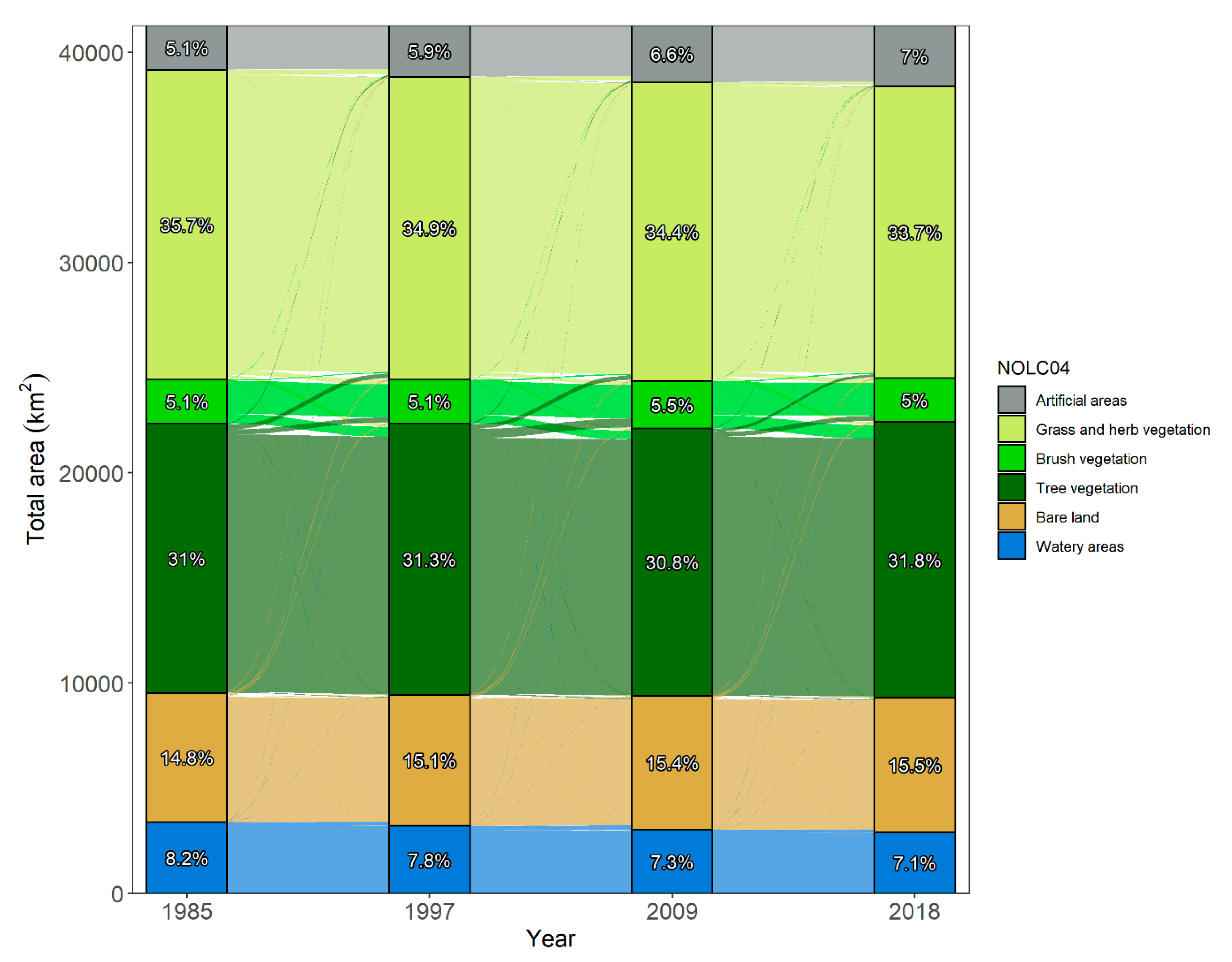
3.1. Land Cover Change

Switzerland underwent a change in LC Principal Domain of 5.41% from 1985–1997, 5.45% from 1997–2009 and 5.12% from 2009–2018. This figure rises to 10.7% between 1985 and 2018 (Figure 4). Concerning LC Basic Categories, 16.2% of the total proportion of land changed between 1985 and 2018 and shows a slight continuous increase over the different periods of investigation, with a change of 7.59% during the period 1985–1997, 8.32% during 1997–2009 and 8.68% from 2009 to 2018. Grass and Herb Vegetation and Watery Areas consistently decline in percentage of the total map area from 1985 to 2018 (Table S1).
Tree vegetation, the second largest LC category, experiences the greatest absolute loss (between 1997 and 2009) and gain (between 2009 and 2018) in a time interval from a loss of closed forest, followed by a gain in open forest. The largest changes in terms of total area are between brush and tree vegetation in each time interval (Figure S1).

3.2. Change Intensity over Time

At all levels of LC nomenclature, and for all time intervals considered, the annual intensity of change is greater than the uniform intensity for the study area, indicating that the changes occurring can be considered as relatively fast [44]. The annual rate of LC change is higher in the period from 2009 to 2018, and this pattern can be observed across all regions (Figure 5 and Figure 6). Basic Categories are more dynamic than the Principal Domains, with a greater percentage of the map area undergoing change due to subtle changes within the broader classifications that are more easily triggered. Land Cover is, in general, more dynamic than Land Use on both the national and regional scale. The Western Central Alps are an exception to this, where the annual percentage change in Land Use was greater than for Land Cover in the first two intervals, driven by gains in non-agricultural forests and losses in unproductive areas and alpine grazing areas.

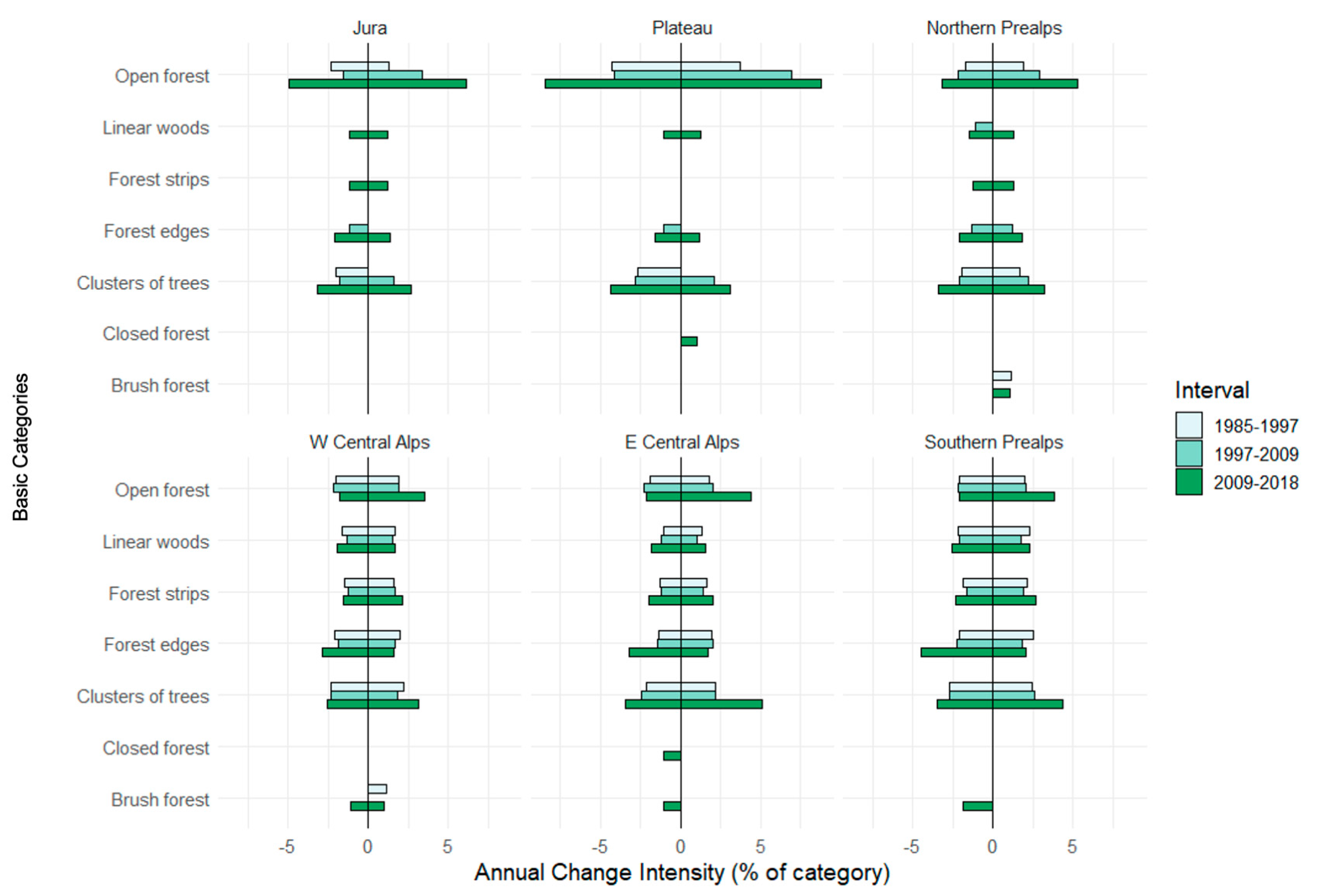
3.3. Category Intensity

As a contrast to gains in buildings that are only above uniform intensity in the first interval, annual percentage losses in the minor categories of artificial areas are greatest in 2009–2018, in all regions (Figure 6). The Jura and Plateau regions show much greater annual change intensities than the alpine regions, driven by changes within vegetated LC classes (Figure 7 and Figure 8).
Changes in most tree vegetation categories are also greatest in this interval across all regions, but to a greater degree in the Jura and Plateau regions where vegetation changes are generally more dynamic (Figure 7 and Figure 8). Watery Areas undergo more minor changes, with fewer regions showing changes above uniform intensity; however, loss of glaciers and perpetual snow can be observed in the Eastern Central Alps and the Southern Alps. Bare Land categories occupy a much larger total surface area in the alpine regions, and this is reflected in the low intensity of change that remains lower than uniform intensity in all intervals.
Greater changes in marginal forest areas, such as Forest Strips and Forest Edges, can be observed in the alpine regions compared to the Plateau and Jura, and a lower rate of change in open forest reflects the difference in management strategies [31].

3.4. Key LC Transitions

A transition between two classes, A and B, can be viewed as a dominant signal of change if class A systematically loses surface to class B, while at the same time class B systematically gains surface from class A [18]. At the national scale, the most important change signals are the gain in Tree Vegetation from Brush Vegetation categories, for which there is a clear increase in the 2009–2018 period compared to other years (Figure 9). The intensity of gain of Tree Vegetation from Brush Vegetation is not equivalent to the intensity of loss from Brush Vegetation to Tree Vegetation, as these values are calculated based on the initial size of the changing category in question.
The transition from Watery Areas to Bare Land reflects the loss of permanent snow and glacier in alpine areas within the Basic Categories. However, the largest transitions are all weighted in one direction. While the loss of Grass and Herb Vegetation to Artificial Areas and the gain of Artificial Areas from Grass and Herb Vegetation are both systematic transitions above the rate of uniform change, the loss of Grass and Herb Vegetation to Artificial Areas occurs at a much higher intensity. As a result, the signals of the change identified are weak.
The central trends identified for the Tree and Brush Vegetation categories are from Brush classes to Tree classes, with the strongest signals of change in the 2009–2018 period being systematic transitions from Shrubs and Brush Meadows to Closed Forest.
At the lower level of thematic precision, alongside the transition from tree to brush vegetation, another important change is a gain of bare land from watery areas. This is observed particularly in the alpine areas where the Basic Categories indicate this is the loss of glaciers and permanent snow.

3.5. Change in Spatial Patterns

Over the whole study period, most pixels show a non-negligible change in the spatial pattern. The highest difference in the spatial pattern is observed in the Plateau and northern Prealps regions, notably in the 1997–2009 period (Figure 10). When grouped by the Basic Categories, all intervals undergo a similar distribution of change, however, more pixels show a JSD value > 0.012, reflecting the higher dynamism of LC change at the higher level of category disaggregation. Amongst the areas of highest distance, the most important changes to the spatial configuration of the landscape can be observed during 1997–2009, primarily in the form of changes towards less dense vegetation, transitioning from closed forest to shrubs, open forest, and clusters of trees.
Between 1985 and 2018, the loss of permanent snow and glaciers produces the highest difference in spatial configuration of the landscape, with major differences at the intersection of the Western and Eastern Central Alps, and the Southern Prealps (Figure 11).

4. Discussion

4.1. Land Cover Dynamics in Switzerland

At the national scale, the gross values of LC gain and loss over the study period would suggest that Switzerland’s landscape is relatively static, with just over 5% of land cover changing in the Principal Domain between each dataset, and low levels of difference in configuration and composition of land cover at the scale of 25 km2. However, exploration of pixel-level statistics shows that the land cover has changed above what would be expected under the hypothesis of random change, and particularly at the levels of higher disaggregation, land cover has been highly dynamic. Furthermore, many of these changes have been equally dynamic in terms of both LC gain and loss, which, while this may be reported as a net persistence in LUCC statistics, indicates a more dynamic landscape. Changes are of a lower magnitude than those reported for recent LU changes [26].
The low values of difference at the landscape scale, however, highlight that LC changes have taken the form of mostly multiple small-scale transformations rather than large contiguous areas. This is further emphasized by the weak, and mostly one-sided results, achieved when exploring the dominant signals of LC change. Change at spatial scales above the pixel level is most important for areas of glacier retreat and loss of permanent snow and ice, reflecting the significant loss of low-altitude snow and ice with climate change [26]. As indicated by official Land Use reporting [26], the transition from glacier to newly vegetated areas, while reported in the literature [47], is not yet significant enough to be detected through LUCC intensity analysis. The low-absolute levels of differences reported, however, reflect that these areas remain relatively intact, with loss occurring at the edges of the glaciers, rather than in the form of fragmentation of the landscape.
While built surfaces have shown to continue to increase the surface area with each survey period, intensity analysis confirms the published results showing the rate at which these surfaces’ gain area has decreased [26]. The continued expansion of forest areas over former agricultural surfaces in alpine areas [26] and observed ‘greening’ of the plateau region [8] is also reflected.
All regions undergo a higher annual rate of land cover change between the 2009 and 2018 datasets. At the category level, spatial disaggregation of change is more evident, with the Jura and Plateau regions showing highly dynamic rates of change for vegetated categories. Investigation at the level of category transitions show that the key transition occurring within the Plateau region is to and from the closed forest, a trend which is more important in this region compared to the alpine regions where a relative change to expansive forest areas is less dramatic. The similarity in the intensity of gain and loss in the forest areas of the plateau region reflects the findings of the National Forest Inventory, which reports that the total forest area in this area was stable over the study period. The results presented indicate that the reason for the increased rate of change in the final time interval is due, in part, to the transition from brush vegetation to forest classes. However, this increased rate of change in the Plateau region is at odds with reports of the forested land in this region remaining static in recent years [26]. This increased rate of transition could indicate the emergence of new pressures on LC, or a change of intensity of certain pressures [19] that are not yet occurring at a magnitude detectable in absolute LC change.

4.2. The Need for Higher Spatial & Temporal National Land Cover Data

Accurate, reliable, and timely land cover data are crucial for the understanding and modeling of environmental processes [48], as well as for informing socio-economic policy at the right pace for action [49]. As such, the low update frequency of the ArealStatistik is at odds with the data needs for quantifying variables that are known to be as dynamic as land cover and land use [50]. Analysis of annual land cover maps would facilitate a greater understanding of the processes and drivers that result in LUCC [19,51] and allow for consideration of both subtle and rapid changes that can both indicate changes to LUC pressures.
Understanding ecological processes, including disturbances and climate feedback, which are key to the comprehensive assessment of the drivers and pressures facing the environment, requires the utilization of multiple time-steps of annual or even sub-annual land cover data [51,52]. This need is particularly evident considering the increased rate of change identified in some categories during the 2009–2018 interval and the difficulty in establishing a cause of this.
The knowledge gap surrounding the dynamics of LUCC in Switzerland is, to an extent, perpetuated by the limited temporal resolution of the datasets used. At the current resolution, the question remains whether the observed increased intensity of change between the two most recent survey periods is indicative of real changes in Land Cover change drivers, or merely an artifact of the periodicity of sampling that may be less relevant upon production of the next LC dataset. The analysis of absolute trends over the 9–12 years intervals presented here provides an indication of changes or persistence, however, there may be intermediate growths and declines in categories that manifest as an overall non-trend and are not effectively captured using the ArealStatistik. This hinders the effective use of time-series change detection and trend algorithms such as Breaks For Additive Season and Trend (BFAST) [53,54,55], Continuous Change Detection and Classification (CCDC), or LandTrendr [56]. Moreover, the timing of the aerial image acquisition can have an influence on the consistency of classification and observed changes. Indeed, for the last survey covering the period 2013 to 2018, it took 6 years to cover the entire country, meaning that each year, approximately one-sixth of the territory is covered and processed according to the schema of acquisition presented on https://www.bfs.admin.ch/bfs/fr/home/statistiques/espace-environnement/enquetes/area/bases-donnees/photographies-aeriennes.html, accessed on 29 May 2023. Once the entire country is covered, the dataset is then released for the given survey period. With such a sequential approach, lots of LUC change can occur from the time the first tiles are processed until the last one. Consequently, LUC transitions can be missed, lowering the proportion of observed changes. This reinforces the need for yearly, consistent, accurate, and high-resolution LC maps for Switzerland.
It can be further argued that analysis of LUCC benefits from a consideration of different spatial scales, as landscape patterns sometimes show a high degree of variability depending on the spatial scale used [19], and dynamic but small-sized landscape areas can contribute greatly to observed changes. The relatively coarse spatial resolution of the ArealStatistik may mean that this dynamism is not fully captured. Refining LC data to a smaller spatial resolution facilitates the capture of processes occurring at the scale of human activity [57].
Recent efforts to downscale LUC data for Switzerland have improved the spatial resolution to 25 m, however, there remains a gap in the temporal dimension of datasets produced [21]. Several initiatives exist to produce global land cover datasets at high-spatial and temporal resolutions [58,59,60], however, their use at a local-national scale can be limited by variability in accuracy across space and a relatively low number of thematic classes compared to national datasets [48,61].

4.3. Perspectives

Although the ArealStatistik is useful and, thematically, more precise than commonly used classifications, it suffers from various limitations (i.e., spatial (1-hectare) and temporal (every 6 years) resolutions for consistent environmental monitoring. Consequently, this survey-based method constrains researchers and policymakers to work with data that do not necessarily reflect on the ground realities impending the ability to correctly capture detailed landscape features, qualities, particularities, and configurations, as well as the entire dynamics of change (e.g., low temporal granularity allows for capturing slow onset changes and not the potential rapid change of the landscape).
The big and constantly increasing amount of freely available EO data (Big Earth Data [62,63]) with enhanced temporal, spatial, and spectral resolution, together with rapid development in remote sensing data storage, handling, and processing technologies (e.g., Data Cube, Machine Learning), offers new opportunities for LUC mapping at finer spatial, temporal, and thematic resolutions [57,64,65]. The increasing availability of open-access, high-resolution remote sensing data has vastly increased the potential for the development of land cover datasets from local to global scales [50]. Satellite imagery provides a consistent dataset of earth observations that is spatially continuous and contains the temporal resolution necessary to identify classes with strong temporal dynamics [48,61].
However, among the major identified issues concerning the increase in spatial and temporal resolution when producing LC data are (1) the possibility to discriminate a higher number of features, which, at the same time, leads to a general increase of variability in LC classes and, consequently, a decrease in accuracy level when using traditional classification methods; and (2) the lack of ground-reference data for validating the results [66,67,68].
To overcome these issues, Machine/Deep Learning (ML/DL) algorithms (e.g., convolutional neural networks, gradient-boosted trees) have demonstrated their potential to generate results of higher accuracy than those produced with parametric classifiers, being able to deal with higher dimensionality (e.g., space and time) and map classes with complex characteristics. This allows for the development of supervised classification models that correlate different information (spectral, spatial, temporal, and ancillary) to an area of interest [69].
The “ArealStatistik” is a unique dataset set providing 4 million ground-referenced points for each period (4 in total). Part of this data set can be used for both the train, test, and validate stages of classification. For training, this can be used as reference data to identify a sample of pixels of known classes; then in the allocation phase, pixels will be assigned to a given class according to their statistical similarities; finally, the accuracy of the classification can be tested by comparing a sample of pixels in both classified and reference data and generate an error matrix [70,71]. Recent advances in machine learning techniques, such as multitask learning, multi-instance learning, and multiview learning, could be also explored to tackle issues such as landscape heterogeneity in space and time (e.g., vegetation), potential lack of training data, and rarity of land cover change while developing a suitable model for LC and LCC [72,73].
Therefore, to improve the spatial and temporal resolution of land cover data of Switzerland, while keeping the thematic richness of the “Arealstatistik”, the availability of more than 39 years of satellite EO Analysis Ready Data over Switzerland, made available by the Swiss Data Cube (https://www.swissdatacube.ch, accessed on 29 May 2023) [74,75,76], together with ML/DL techniques [77,78], allow the envisioning of innovative approaches to produce a yearly 10/30 m consistent time-series of LC and its changes, informing on class stability and transitions [79,80], to support effective national environmental monitoring [81,82].

5. Conclusions

The results presented here highlight the continued dynamism of LC in Switzerland over a period of 33 years. Assessment of spatial configuration identified low degrees of change across most of Switzerland in all time periods assessed, reflecting the many pixel-level transitions which have occurred. The findings, however, reflect the difficulty in assessing systematic LC change at the national and regional level, as the large range of small, spatially dispersed and gradual trends required aggregation to be detected, but this means that any locally important drivers or trends may have been masked. A clear dynamic over the study period is the high rates of annual change in low-growing Brush Vegetation, in the form of meadows and shrubs in the low-altitude regions, for which an increased intensity of change was detected in recent years. This could be a sign that drivers of LC change are evolving, but with the currently available data, it is not possible to deduce the drivers of this. The increased rate of transition between Brush Vegetation and Tree Vegetation LC classes in the Jura and Plateau regions are more dynamic, as there is a greater human influence in LUC, but there is not a clear pathway at the national or regional scale as to why shrub vegetation would be changing more than it has previously. Trends such as an increased rate of change to and from forest LC classes can be identified, but an understanding of reasons behind this is limited by infrequent updates to LC data.
This work highlights that although the ArealStatistik is very useful thanks to its thematic richness, neither its low spatial resolution or update frequency allows for providing accurate and timely information to depict and understand the detailed dynamics of LCC and the related impact across the country. Accurate LC change assessment and effective LC projections require higher spatial (e.g., 10–30 m) and temporal (e.g., yearly) data products to build consistent time series. This restricts the comprehensive understanding of the gains and losses of LUC types, including the magnitudes, locations, and timings of transitions. Understanding the drivers of observed changes, particularly a potential increase in the rate of change towards Tree Vegetation classes, is important to inform both reflections on past environmental policies and the development of future management strategies. The ability to understand these drivers would benefit from a high-resolution annual LC dataset. Advances in ML/DL techniques, combined with increased availability of satellite data time series available in the Swiss Data Cube, present the potential for the development of such a dataset, in combination with the ArealStatistik, which provides a geographically specific LC classification scheme.

Supplementary Materials

The following supporting information can be downloaded at: https://www.mdpi.com/article/10.3390/land12071386/s1, Figure S1: Sankey diagram showing change in proportion of NOLC04 Basic Categories. The legend is the same as Figure 11. Figure S2: Land Use interval intensity (difference from uniform intensity); Table S1: Cross Tabulation Matrix for LC Principal Domains, for the periods 1985–1997, 1997–2009, and 2009–2018.

Author Contributions

Conceptualization, I.N.T. and G.G.; methodology, I.N.T.; formal analysis, I.N.T.; data curation, I.N.T.; writing—original draft preparation, I.N.T. and G.G.; writing—review and editing, all; visualization, I.N.T. and G.G.; supervision, G.G.; project administration. All authors have read and agreed to the published version of the manuscript.

Funding

This research received no external funding.

Data Availability Statement

Publicly available datasets were analyzed in this study. These data can be found here: Land Use Statistics (https://www.bfs.admin.ch/bfs/de/home/statistiken/raum-umwelt/erhebungen/area.html, accessed on 10 October 2022); National and bio geographical regions (https://www.swisstopo.admin.ch/en/geodata/landscape/boundaries3d.html, accessed on 10 October 2022).

Acknowledgments

The Swiss Federal Office for Statistics (FSO) is gratefully acknowledged for making the input data freely available.

Conflicts of Interest

The authors declare no conflict of interest.

References

  1. UNCCD. Global Land Outlook: Land Restoration for Recovery and Resilience; UNCCD: Bonn, Germany, 2022; p. 204. [Google Scholar]
  2. Metternicht, G.; Akhtar-Schuster, M.; Castillo, V. Implementing Land Degradation Neutrality: From Policy Challenges to Policy Opportunities for National Sustainable Development. Environ. Sci. Policy 2019, 100, 189–191. [Google Scholar] [CrossRef]
  3. Comber, A.J. Land Use or Land Cover? J. Land Use Sci. 2008, 3, 199–201. [Google Scholar] [CrossRef]
  4. Bojinski, S.; Verstraete, M.; Peterson, T.C.; Richter, C.; Simmons, A.; Zemp, M. The Concept of Essential Climate Variables in Support of Climate Research, Applications, and Policy. Bull. Am. Meteorol. Soc. 2014, 95, 1431–1443. [Google Scholar] [CrossRef] [Green Version]
  5. Jetz, W.; McGeoch, M.A.; Guralnick, R.; Ferrier, S.; Beck, J.; Costello, M.J.; Fernandez, M.; Geller, G.N.; Keil, P.; Merow, C.; et al. Essential Biodiversity Variables for Mapping and Monitoring Species Populations. Nat. Ecol. Evol. 2019, 3, 539–551. [Google Scholar] [CrossRef] [Green Version]
  6. Pereira, H.M.; Leadley, P.W.; Proenca, V.; Alkemade, R.; Scharlemann, J.P.W.; Fernandez-Manjarres, J.F.; Araujo, M.B.; Balvanera, P.; Biggs, R.; Cheung, W.W.L.; et al. Scenarios for Global Biodiversity in the 21st Century. Science 2010, 330, 1496–1501. [Google Scholar] [CrossRef] [PubMed] [Green Version]
  7. Knöfel, P.; Hovenbitzer, M. Introduction of the German Landscape Change Detection Service. In Proceedings of the 2018 IEEE IGARSS Conference, Valencia, Spain, 22–27 July 2018; pp. 806–809. [Google Scholar]
  8. Hersperger, A.M.; Bürgi, M. Going beyond Landscape Change Description: Quantifying the Importance of Driving Forces of Landscape Change in a Central Europe Case Study. Land Use Policy 2009, 26, 640–648. [Google Scholar] [CrossRef]
  9. Dale, V.H. The Relationship Between Land-Use Change and Climate Change. Ecol. Appl. 1997, 7, 753–769. [Google Scholar] [CrossRef]
  10. Foley, J.A.; DeFries, R.; Asner, G.P.; Barford, C.; Bonan, G.; Carpenter, S.R.; Chapin, F.S.; Coe, M.T.; Daily, G.C.; Gibbs, H.K.; et al. Global Consequences of Land Use. Science 2005, 309, 570–574. [Google Scholar] [CrossRef] [Green Version]
  11. Chaves, M.E.D.; Soares, A.R.; Mataveli, G.A.V.; Sánchez, A.H.; Sanches, I.D. A Semi-Automated Workflow for LULC Mapping via Sentinel-2 Data Cubes and Spectral Indices. Automation 2023, 4, 94–109. [Google Scholar] [CrossRef]
  12. Grêt-Regamey, A.; Altwegg, J.; Sirén, E.A.; van Strien, M.J.; Weibel, B. Integrating Ecosystem Services into Spatial Planning—A Spatial Decision Support Tool. Landsc. Urban Plan. 2017, 165, 206–219. [Google Scholar] [CrossRef] [Green Version]
  13. Hermosilla, T.; Wulder, M.A.; White, J.C.; Coops, N.C. Land Cover Classification in an Era of Big and Open Data: Optimizing Localized Implementation and Training Data Selection to Improve Mapping Outcomes. Remote Sens. Environ. 2022, 268, 112780. [Google Scholar] [CrossRef]
  14. Munsi, M.; Malaviya, S.; Oinam, G.; Joshi, P.K. A Landscape Approach for Quantifying Land-Use and Land-Cover Change (1976–2006) in Middle Himalaya. Reg. Environ. Chang. 2010, 10, 145–155. [Google Scholar] [CrossRef]
  15. Rutherford, G.N.; Bebi, P.; Edwards, P.J.; Zimmermann, N.E. Assessing Land-Use Statistics to Model Land Cover Change in a Mountainous Landscape in the European Alps. Ecol. Model. 2008, 212, 460–471. [Google Scholar] [CrossRef]
  16. Romero-Ruiz, M.H.; Flantua, S.G.A.; Tansey, K.; Berrio, J.C. Landscape Transformations in Savannas of Northern South America: Land Use/Cover Changes since 1987 in the Llanos Orientales of Colombia. Appl. Geogr. 2012, 32, 766–776. [Google Scholar] [CrossRef]
  17. Pontius, R.G.; Shusas, E.; McEachern, M. Detecting Important Categorical Land Changes While Accounting for Persistence. Agric. Ecosyst. Environ. 2004, 101, 251–268. [Google Scholar] [CrossRef]
  18. Braimoh, A.K. Random and Systematic Land-Cover Transitions in Northern Ghana. Agric. Ecosyst. Environ. 2006, 113, 254–263. [Google Scholar] [CrossRef]
  19. Teixeira, Z.; Teixeira, H.; Marques, J.C. Systematic Processes of Land Use/Land Cover Change to Identify Relevant Driving Forces: Implications on Water Quality. Sci. Total Environ. 2014, 470–471, 1320–1335. [Google Scholar] [CrossRef] [Green Version]
  20. Cojoc, E.I.; Postolache, C.; Olariu, B.; Beierkuhnlein, C. Effects of Anthropogenic Fragmentation on Primary Productivity and Soil Carbon Storage in Temperate Mountain Grasslands. Environ. Monit. Assess. 2016, 188, 653. [Google Scholar] [CrossRef]
  21. Giuliani, G.; Rodila, D.; Külling, N.; Maggini, R.; Lehmann, A. Downscaling Switzerland Land Use/Land Cover Data Using Nearest Neighbors and an Expert System. Land 2022, 11, 615. [Google Scholar] [CrossRef]
  22. Artmann, M.; Bastian, O.; Grunewald, K. Using the Concepts of Green Infrastructure and Ecosystem Services to Specify Leitbilder for Compact and Green Cities—The Example of the Landscape Plan of Dresden (Germany). Sustainability 2017, 9, 198. [Google Scholar] [CrossRef] [Green Version]
  23. Bateman, I.J.; Harwood, A.R.; Mace, G.M.; Watson, R.T.; Abson, D.J.; Andrews, B.; Binner, A.; Crowe, A.; Day, B.H.; Dugdale, S.; et al. Bringing Ecosystem Services into Economic Decision-Making: Land Use in the United Kingdom. Science 2013, 341, 45–50. [Google Scholar] [CrossRef] [PubMed]
  24. Johnson, J.A.; Jones, S.K.; Wood, S.L.R.; Chaplin-Kramer, R.; Hawthorne, P.L.; Mulligan, M.; Pennington, D.; DeClerck, F.A. Mapping Ecosystem Services to Human Well-Being: A Toolkit to Support Integrated Landscape Management for the SDGs. Ecol. Appl. 2019, 29, e01985. [Google Scholar] [CrossRef]
  25. Swiss Federal Statistical Office. The Changing Face of Land Use: Land Use Statistics of Switzerland; SFO: Neuchâtel, Switzerland, 2001; p. 32.
  26. Beyeler, N.; Douard, R.; Jeannet, A.; Willi-Tobler, L.; Weibel, F. Land Use in Switzerland: Results of the Swiss Land Use Statistics 2018; Land use in Switzerland; Bundesamt für Statistik (BFS): Neuchâtel, Switzerland, 2021; ISBN 978-3-303-02130-9. [Google Scholar]
  27. Altwegg, D. L’utilisation du sol en Suisse; Bundesamt für Statistik (BFS): Neuchâtel, Switzerland, 2015; ISBN 978-3-303-02126-2. [Google Scholar]
  28. Bolliger, J.; Hagedorn, F.; Leifeld, J.; Böhl, J.; Zimmermann, S.; Soliva, R.; Kienast, F. Effects of Land-Use Change on Carbon Stocks in Switzerland. Ecosystems 2008, 11, 895–907. [Google Scholar] [CrossRef]
  29. Bolliger, J.; Kienast, F.; Soliva, R.; Rutherford, G. Spatial Sensitivity of Species Habitat Patterns to Scenarios of Land Use Change (Switzerland). Landsc. Ecol. 2007, 22, 773–789. [Google Scholar] [CrossRef] [Green Version]
  30. Price, B.; Kienast, F.; Seidl, I.; Ginzler, C.; Verburg, P.H.; Bolliger, J. Future Landscapes of Switzerland: Risk Areas for Urbanisation and Land Abandonment. Appl. Geogr. 2015, 57, 32–41. [Google Scholar] [CrossRef]
  31. Loran, C.; Munteanu, C.; Verburg, P.H.; Schmatz, D.R.; Bürgi, M.; Zimmermann, N.E. Long-Term Change in Drivers of Forest Cover Expansion: An Analysis for Switzerland (1850–2000). Reg. Environ. Chang. 2017, 17, 2223–2235. [Google Scholar] [CrossRef]
  32. Pazúr, R.; Huber, N.; Weber, D.; Ginzler, C.; Price, B. A National Extent Map of Cropland and Grassland for Switzerland Based on Sentinel-2 Data. Earth Syst. Sci. Data 2022, 14, 295–305. [Google Scholar] [CrossRef]
  33. Price, B.; Huber, N.; Nussbaumer, A.; Ginzler, C. The Habitat Map of Switzerland: A Remote Sensing, Composite Approach for a High Spatial and Thematic Resolution Product. Remote Sens. 2023, 15, 643. [Google Scholar] [CrossRef]
  34. Bär, V.; Akinyemi, F.O.; Ifejika Speranza, C. Land Cover Degradation in the Reference and Monitoring Periods of the SDG Land Degradation Neutrality Indicator for Switzerland. Ecol. Indic. 2023, 151, 110252. [Google Scholar] [CrossRef]
  35. Gómez Giménez, M.; de Jong, R.; Keller, A.; Rihm, B.; Schaepman, M.E. Studying the Influence of Nitrogen Deposition, Precipitation, Temperature, and Sunshine in Remotely Sensed Gross Primary Production Response in Switzerland. Remote Sens. 2019, 11, 1135. [Google Scholar] [CrossRef] [Green Version]
  36. Gonseth, Y.; Wohlgemuth, W.; Sansonnens, B.; Buttler, A. Les Régions Biogéographiques de La Suisse—Explications et Division Standard; Cahier de l’Environnement; Office Fédéral de l’Environnement, des Forêts et du Paysage: Bern, The Switzerland, 2001. [Google Scholar]
  37. Vittoz, P.; Cherix, D.; Gonseth, Y.; Lubini, V.; Maggini, R.; Zbinden, N.; Zumbach, S. Climate Change Impacts on Biodiversity in Switzerland: A Review. J. Nat. Conserv. 2013, 21, 154–162. [Google Scholar] [CrossRef]
  38. NCCS. CH2018—Climate Scenarios for Switzerland, Technical Report; National Centre for Climate Services: Zurich, Switzerland, 2018; p. 271. [Google Scholar]
  39. R Core Team. R: A Language and Environment for Statistical Computing; R Foundation for Statistical Computing: Vienna, Austria, 2021. [Google Scholar]
  40. Van Rossum, G.; Drake, F.L. Python 3 Reference Manual; CreateSpace: Scotts Valley, CA, USA, 2009; ISBN 1-4414-1269-7. [Google Scholar]
  41. Ridd, M.K.; Liu, J. A Comparison of Four Algorithms for Change Detection in an Urban Environment. Remote Sens. Environ. 1998, 63, 95–100. [Google Scholar] [CrossRef]
  42. Mas, J.-F. Monitoring Land-Cover Changes: A Comparison of Change Detection Techniques. Int. J. Remote Sens. 1999, 20, 139–152. [Google Scholar] [CrossRef]
  43. Cuba, N. Research Note: Sankey Diagrams for Visualizing Land Cover Dynamics. Landsc. Urban Plan. 2015, 139, 163–167. [Google Scholar] [CrossRef]
  44. Aldwaik, S.Z.; Pontius, R.G. Intensity Analysis to Unify Measurements of Size and Stationarity of Land Changes by Interval, Category, and Transition. Landsc. Urban Plan. 2012, 106, 103–114. [Google Scholar] [CrossRef]
  45. Nowosad, J. Motif: An Open-Source R Tool for Pattern-Based Spatial Analysis. Landsc. Ecol. 2021, 36, 29–43. [Google Scholar] [CrossRef]
  46. Nowosad, J.; Stepinski, T.F.; Netzel, P. Global Assessment and Mapping of Changes in Mesoscale Landscapes: 1992–2015. Int. J. Appl. Earth Obs. Geoinf. 2019, 78, 332–340. [Google Scholar] [CrossRef] [Green Version]
  47. Bolton, D.K.; Coops, N.C.; Hermosilla, T.; Wulder, M.A.; White, J.C. Evidence of Vegetation Greening at Alpine Treeline Ecotones: Three Decades of Landsat Spectral Trends Informed by Lidar-Derived Vertical Structure. Environ. Res. Lett. 2018, 13, 084022. [Google Scholar] [CrossRef]
  48. Verde, N.; Kokkoris, I.P.; Georgiadis, C.; Kaimaris, D.; Dimopoulos, P.; Mitsopoulos, I.; Mallinis, G. National Scale Land Cover Classification for Ecosystem Services Mapping and Assessment, Using Multitemporal Copernicus EO Data and Google Earth Engine. Remote Sens. 2020, 12, 3303. [Google Scholar] [CrossRef]
  49. Gómez, C.; White, J.C.; Wulder, M.A. Optical Remotely Sensed Time Series Data for Land Cover Classification: A Review. ISPRS J. Photogramm. Remote Sens. 2016, 116, 55–72. [Google Scholar] [CrossRef] [Green Version]
  50. Ban, Y.F.; Gong, P.; Gini, C. Global Land Cover Mapping Using Earth Observation Satellite Data: Recent Progresses and Challenges. ISPRS J. Photogramm. Remote Sens. 2015, 103, 1–6. [Google Scholar] [CrossRef] [Green Version]
  51. Kennedy, R.E.; Andréfouët, S.; Cohen, W.B.; Gómez, C.; Griffiths, P.; Hais, M.; Healey, S.P.; Helmer, E.H.; Hostert, P.; Lyons, M.B.; et al. Bringing an Ecological View of Change to Landsat-based Remote Sensing. Front. Ecol. Environ. 2014, 12, 339–346. [Google Scholar] [CrossRef] [PubMed]
  52. Luo, Y.; Lü, Y.; Fu, B.; Zhang, Q.; Li, T.; Hu, W.; Comber, A. Half Century Change of Interactions among Ecosystem Services Driven by Ecological Restoration: Quantification and Policy Implications at a Watershed Scale in the Chinese Loess Plateau. Sci. Total Environ. 2019, 651, 2546–2557. [Google Scholar] [CrossRef] [PubMed] [Green Version]
  53. Verbesselt, J.; Hyndman, R.; Newnham, G.; Culvenor, D. Detecting Trend and Seasonal Changes in Satellite Image Time Series. Remote Sens. Environ. 2010, 114, 106–115. [Google Scholar] [CrossRef]
  54. Verbesselt, J.; Hyndman, R.; Zeileis, A.; Culvenor, D. Phenological Change Detection While Accounting for Abrupt and Gradual Trends in Satellite Image Time Series. Remote Sens. Environ. 2010, 114, 2970–2980. [Google Scholar] [CrossRef] [Green Version]
  55. Verbesselt, J.; Zeileis, A.; Herold, M. Near Real-Time Disturbance Detection Using Satellite Image Time Series. Remote Sens. Environ. 2012, 123, 98–108. [Google Scholar] [CrossRef]
  56. Pasquarella, V.J.; Arévalo, P.; Bratley, K.H.; Bullock, E.L.; Gorelick, N.; Yang, Z.; Kennedy, R.E. Demystifying LandTrendr and CCDC Temporal Segmentation. Int. J. Appl. Earth Obs. Geoinf. 2022, 110, 102806. [Google Scholar] [CrossRef]
  57. Wulder, M.A.; Coops, N.C.; Roy, D.P.; White, J.C.; Hermosilla, T. Land Cover 2.0. Int. J. Remote Sens. 2018, 39, 4254–4284. [Google Scholar] [CrossRef] [Green Version]
  58. Venter, Z.S.; Sydenham, M.A.K. Continental-Scale Land Cover Mapping at 10 m Resolution Over Europe (ELC10). Remote Sens. 2021, 13, 2301. [Google Scholar] [CrossRef]
  59. Brown, C.F.; Brumby, S.P.; Guzder-Williams, B.; Birch, T.; Hyde, S.B.; Mazzariello, J.; Czerwinski, W.; Pasquarella, V.J.; Haertel, R.; Ilyushchenko, S.; et al. Dynamic World, Near Real-Time Global 10 m Land Use Land Cover Mapping. Sci. Data 2022, 9, 251. [Google Scholar] [CrossRef]
  60. Venter, Z.S.; Barton, D.N.; Chakraborty, T.; Simensen, T.; Singh, G. Global 10 m Land Use Land Cover Datasets: A Comparison of Dynamic World, World Cover and Esri Land Cover. Remote Sens. 2022, 14, 4101. [Google Scholar] [CrossRef]
  61. Inglada, J.; Vincent, A.; Arias, M.; Tardy, B.; Morin, D.; Rodes, I. Operational High Resolution Land Cover Map Production at the Country Scale Using Satellite Image Time Series. Remote Sens. 2017, 9, 95. [Google Scholar] [CrossRef] [Green Version]
  62. Guo, H.; Wang, L.; Liang, D. Big Earth Data from Space: A New Engine for Earth Science. Sci. Bull. 2016, 61, 505–513. [Google Scholar] [CrossRef]
  63. Guo, H.; Nativi, S.; Liang, D.; Craglia, M.; Wang, L.; Schade, S.; Corban, C.; He, G.; Pesaresi, M.; Li, J.; et al. Big Earth Data Science: An Information Framework for a Sustainable Planet. Int. J. Digit. Earth 2020, 13, 743–767. [Google Scholar] [CrossRef] [Green Version]
  64. Feng, M.; Bai, Y. A Global Land Cover Map Produced through Integrating Multi-Source Datasets. Big Earth Data 2019, 3, 191–219. [Google Scholar] [CrossRef] [Green Version]
  65. Owers, C.J.; Lucas, R.M.; Clewley, D.; Planque, C.; Punalekar, S.; Tissott, B.; Chua, S.M.T.; Bunting, P.; Mueller, N.; Metternicht, G. Living Earth: Implementing National Standardised Land Cover Classification Systems for Earth Observation in Support of Sustainable Development. Big Earth Data 2021, 5, 368–390. [Google Scholar] [CrossRef]
  66. Talukdar, S.; Singha, P.; Mahato, S.; Shahfahad; Pal, S.; Liou, Y.-A.; Rahman, A. Land-Use Land-Cover Classification by Machine Learning Classifiers for Satellite Observations—A Review. Remote Sens. 2020, 12, 1135. [Google Scholar] [CrossRef] [Green Version]
  67. Papoutsis, I.; Bountos, N.I.; Zavras, A.; Michail, D.; Tryfonopoulos, C. Benchmarking and Scaling of Deep Learning Models for Land Cover Image Classification. ISPRS J. Photogramm. Remote Sens. 2023, 195, 250–268. [Google Scholar] [CrossRef]
  68. Santos, L.A.; Ferreira, K.; Picoli, M.; Camara, G.; Zurita-Milla, R.; Augustijn, E.-W. Identifying Spatiotemporal Patterns in Land Use and Cover Samples from Satellite Image Time Series. Remote Sens. 2021, 13, 974. [Google Scholar] [CrossRef]
  69. Maxwell, A.E.; Warner, T.A.; Fang, F. Implementation of Machine-Learning Classification in Remote Sensing: An Applied Review. Int. J. Remote Sens. 2018, 39, 2784–2817. [Google Scholar] [CrossRef] [Green Version]
  70. Olofsson, P.; Foody, G.M.; Herold, M.; Stehman, S.V.; Woodcock, C.E.; Wulder, M.A. Good Practices for Estimating Area and Assessing Accuracy of Land Change. Remote Sens. Environ. 2014, 148, 42–57. [Google Scholar] [CrossRef]
  71. Olofsson, P.; Foody, G.M.; Stehman, S.V.; Woodcock, C.E. Making Better Use of Accuracy Data in Land Change Studies: Estimating Accuracy and Area and Quantifying Uncertainty Using Stratified Estimation. Remote Sens. Environ. 2013, 129, 122–131. [Google Scholar] [CrossRef]
  72. Pandey, P.C.; Koutsias, N.; Petropoulos, G.P.; Srivastava, P.K.; Dor, E.B. Land Use/Land Cover in View of Earth Observation: Data Sources, Input Dimensions, and Classifiers—A Review of the State of the Art. Geocarto Int. 2019, 36, 957–988. [Google Scholar] [CrossRef]
  73. Zhu, X.X.; Tuia, D.; Mou, L.; Xia, G.S.; Zhang, L.; Xu, F.; Fraundorfer, F. Deep Learning in Remote Sensing: A Comprehensive Review and List of Resources. IEEE Geosci. Remote Sens. Mag. 2017, 5, 8–36. [Google Scholar] [CrossRef] [Green Version]
  74. Giuliani, G.; Chatenoux, B.; Bono, A.D.; Rodila, D.; Richard, J.-P.; Allenbach, K.; Dao, H.; Peduzzi, P. Building an Earth Observations Data Cube: Lessons Learned from the Swiss Data Cube (SDC) on Generating Analysis Ready Data (ARD). Big Earth Data 2017, 1, 100–117. [Google Scholar] [CrossRef] [Green Version]
  75. Giuliani, G.; Cazeaux, H.; Burgi, P.-Y.; Poussin, C.; Richard, J.-P.; Chatenoux, B. SwissEnvEO: A FAIR National Environmental Data Repository for Earth Observation Open Science. Data Sci. J. 2021, 20, 22. [Google Scholar] [CrossRef]
  76. Chatenoux, B.; Richard, J.-P.; Small, D.; Roeoesli, C.; Wingate, V.; Poussin, C.; Rodila, D.; Peduzzi, P.; Steinmeier, C.; Ginzler, C.; et al. The Swiss Data Cube, Analysis Ready Data Archive Using Earth Observations of Switzerland. Sci. Data 2021, 8, 295. [Google Scholar] [CrossRef]
  77. Simoes, R.; Camara, G.; Queiroz, G.; Souza, F.; Andrade, P.R.; Santos, L.; Carvalho, A.; Ferreira, K. Satellite Image Time Series Analysis for Big Earth Observation Data. Remote Sens. 2021, 13, 2428. [Google Scholar] [CrossRef]
  78. Giuliani, G.; Camara, G.; Killough, B.; Minchin, S. Earth Observation Open Science: Enhancing Reproducible Science Using Data Cubes. Data 2019, 4, 147. [Google Scholar] [CrossRef] [Green Version]
  79. Woodcock, C.E.; Loveland, T.R.; Herold, M.; Bauer, M.E. Transitioning from Change Detection to Monitoring with Remote Sensing: A Paradigm Shift. Remote Sens. Environ. 2019, 238, 111558. [Google Scholar] [CrossRef]
  80. Arévalo, P.; Bullock, E.L.; Woodcock, C.E.; Olofsson, P. A Suite of Tools for Continuous Land Change Monitoring in Google Earth Engine. Front. Clim. 2020, 2, 576740. [Google Scholar] [CrossRef]
  81. Giuliani, G.; Egger, E.; Italiano, J.; Poussin, C.; Richard, J.-P.; Chatenoux, B. Essential Variables for Environmental Monitoring: What Are the Possible Contributions of Earth Observation Data Cubes? Data 2020, 5, 100. [Google Scholar] [CrossRef]
  82. Lehmann, A.; Mazzetti, P.; Santoro, M.; Nativi, S.; Masò, J.; Serral, I.; Spengler, D.; Niamir, A.; Lacroix, P.; Ambrosone, M.; et al. Essential Earth Observation Variables for High-Level Multi-Scale Indicators and Policies. Environ. Sci. Policy 2022, 131, 105–117. [Google Scholar] [CrossRef]
Figure 1. Graphical summary of processing steps.
Land 12 01386 g001
Figure 2. Biogeographical regions of Switzerland (data from FOEN, 2004).
Land 12 01386 g002
Figure 3. The ArealStatistik visualized on the mapping platform of the Swiss Confederation (https://s.geo.admin.ch/9e445b6a6c, accessed on 28 March 2023).
Land 12 01386 g003
Figure 4. Sankey diagram showing the change in proportion of NOLC04 Principal Domains. Years of survey are depicted on the x-axis as discrete values. In the column bars, the percentages represent the proportion of each class, and the flows between bars show the transition of categories between dates as well as the proportion of change.
Land 12 01386 g004
Figure 5. Land cover interval intensity (difference from uniform intensity) for the Principal Domains (A) and Basic Categories (B). The intensity is for the overall change in the map between the time intervals shown in different shading/color in the columns/bars, according to the legend at the right.
Land 12 01386 g005
Figure 6. Category intensity change of NOLC04 Principal Domains between survey periods. The dashed line indicates uniform intensity from the overall change. Each pair of graphs represent gains (A,C,E) and losses (B,D,F) between the periods of 1985–1997, 1997–2009, and 2009–2018.
Land 12 01386 g006
Figure 7. Category level change intensities (difference from uniform intensity) for Basic Categories within the Brush Vegetation Principal Domain.
Land 12 01386 g007
Figure 8. Category level change intensities (difference from uniform intensity) for Basic Categories within the Tree Vegetation Principal Domain.
Land 12 01386 g008
Figure 9. Dominant signals of change for Principal Domains at the national level (change intensity as difference from uniform intensity).
Land 12 01386 g009
Figure 10. Spatial dissimilarity between periods 1985–1997 (A), 1997–2008 (B), and 2009–2018 (C) as well as the overall survey period 1985–2018 (D) using the Jensen–Shannon divergence at a 25 km2 resolution for comparison based on NOLC04 Basic Categories. JSD is calculated for groups of 25 pixels which aggregate to 25 km2 tiles.
Land 12 01386 g010
Figure 11. Areas of greatest difference (as JSD) in Basic Categories between 1985 (left) and 2018 (right), ranging from JSD of 0.1 (top left) to 0.08 (bottom right). Each pair of images correspond to selected areas across the alpine region of Switzerland to illustrate some major Land Cover changes.
Land 12 01386 g011
Table 1. Land Cover Classification following the NOLC04 nomenclature.
NOLC04_6 (Principal Domains)NOLC04_27 (Basic Categories)
10—Artificial areas11—Consolidated surfaces
12—Buildings
13—Greenhouses
14—Gardens
15—Lawns
16—Trees in artificial areas
17—Mix of small structures
20—Grass & herb vegetation21—Grass & herb vegetation
30—Brush vegetation31—Shrubs
32—Brush meadows
33—Short-stem fruit trees
34—Vines
35—Permanent garden plants & brush crops
40—Tree vegetation41—Closed forest
42—Forest edges
43—Forest strips
44—Open forest
45—Brush forest
46—Linear woods
47—Clusters of trees
50—Bare land51—Solid rock
52—Granular soil
53—Rocky areas
60—Watery areas61—Water
62—Glacier, perpetual snow
63—Wetlands
64—Reedy marshes
Disclaimer/Publisher’s Note: The statements, opinions and data contained in all publications are solely those of the individual author(s) and contributor(s) and not of MDPI and/or the editor(s). MDPI and/or the editor(s) disclaim responsibility for any injury to people or property resulting from any ideas, methods, instructions or products referred to in the content.

