Integrated PSInSAR and GNSS for 3D Displacement in the Wudongde Area

Abstract

The major limitation of persistent scatterer interferometric synthetic aperture radar (PSInSAR) is that it detects only one- or two-dimensional displacements, such as those in the line of sight (LOS) and azimuth directions, by repeat-pass SAR observations. Three-dimensional (3D) displacement reflects the actual sliding surface and failure mechanism of a slope. To transform LOS deformation into a reliable 3D displacement, a new approach for obtaining the 3D displacement is proposed herein based on the slope deformation ($D_{slope}$). First, the deformation value calculated using the Global Navigation Satellite System (GNSS) as a constraint is used to eliminate the residual deformation of PSInSAR. Then, $D_{slope}$ is obtained from the relationship between $D_{LOS}$ and the slope angle extracted from the digital elevation model (DEM). Finally, according to the geometric relationship between $D_{slope}$ and $D_{LOS}$, a novel approach for calculating 3D displacement is proposed. When comparing the 3D displacement extracted by the proposed method and that from GNSS data in Jinpingzi landslide, the root-mean-square error (RMSE) values were ±2.0 mm, ±2.8 mm, and ±2.6 mm in the vertical, north, and east directions, respectively. The proposed method shows high accuracy in 3D displacement calculation, which can help to determine the failure mechanism of a landslide. This method can be widely used in landslide monitoring in wide areas.

1. Introduction

Three-dimensional (3D) displacement is important for ground surface monitoring and natural hazard assessments of landslides [1], volcanoes [2], and earthquakes [3]. It not only reflects the real kinetic features of landslides directly but also clearly displays the mechanisms of shear surfaces and subsurface processes. Remote sensing has been widely used in landslide monitoring, including digital image correlation [4] and offset tracking [5]. The interferometry synthetic aperture radar (InSAR) technique and global positioning system (GPS) are the most effective tools for monitoring 3D displacement [6,7,8]. The InSAR technique includes persistent scatterer InSAR (PSInSAR), small baseline subset InSAR (SBAS), and burst overlap InSAR (BOI). InSAR has the advantage of long-term and all-weather detection of differences in interferometric images [9]. InSAR can detect surface movements in one-dimensional (1D) deformations along the satellite line of sight (LOS) [10,11]. However, 3D displacements decompose into the vertical (V), north–south (N), and east–west (E) directions, which cannot be obtained from a 1D vector. GPS devices can provide 3D surface deformations with precisions of 1–2 mm in the horizontal direction and 3–4 mm in the vertical direction [12]. However, it is difficult to obtain sufficient data, and the spatial resolution is low. Thus, to acquire 3D displacement in a wide area, the GNSS and digital elevation models (DEMs) as geotechnical models are integrated with InSAR observations to complement each other in their spatial and temporal resolutions.

Many scholars have developed integration methods for GNSS and InSAR to obtain 3D displacements [13,14,15]. Chen et al. applied two external GPS stations to provide constraining data to monitor displacement in Hong Kong [16]. Shi et al. used multiangular SAR and the GNSS to retrieve the 3D displacement history of the Shuping landslide in the Three Gorges area [17]. Xiong et al. proposed an iterative least squares method for virtual observation to constrain 3D displacement using GPS stations interpolated into the spatial density of InSAR points [18]. Ren et al. analyzed the deformation characteristics and mechanism of Zaogutian based on deep-seated gravitational slope deformation. The 3D deformation rate field and time-series displacement were reconstructed according to the InSAR monitoring results and the surface-parallel flow assumption [19]. Hu et al. proposed a weighted least squares method to obtain accurate 3D displacements and balance possible errors in InSAR observations [20]. Applying another ground monitoring method used in landslides, Dematteis et al. (2022) proposed integrating robotic total stations and digital images to calculate the 3D displacement and analyze the kinematic features of landslides [21]. Consequently, the integration of InSAR and the GNSS can be used to obtain a real 3D displacement.

For the above studies, the main categories of methods used to obtain 3D displacements by integrating InSAR and the GNSS can be summarized as follows: (1) GNSS points were used as constraining data to remove motion or elevation errors from multiple-time InSAR (MTI) techniques. At least three different MTI observations were used to measure the LOS and azimuth directions, such as ascending and descending, to transform them into 3D displacements [22,23,24]. (2) The least squares method was used to interpolate the GNSS into the same spatial resolution as the MTI data to solve the 3D displacement, considering and balancing possible errors in the MTI observations [25,26]. (3) Numerical simulation is an effective tool for obtaining continuous 3D displacements. However, this method depends on the reliability and accuracy of the model parameters. In general, the geometric parameters of faults, such as their length, width, depth, strike, and dip, have been used to estimate dip-slip and strike-slip movements [27,28]. However, geological conditions, such as the slope angle and aspect, which have a close relation with landslide sliding, were not considered when calculating the 3D displacement.

In this study, in order to obtain the 3D displacement with high precision in a wide area, a new calculation method is proposed based on $D_{slope}$. GNSS points are used to constrain the PS net during the spatial unwrapping of PSInSAR processing to obtain a high-precision $D_{LOS}$. Moreover, based on the analysis of the relationship between $D_{slope}$, the slope angle, and the aspect, a new approach is proposed to calculate the 3D displacement. Finally, the 3D displacement characteristics and mechanism of the Jinpingzi landslide and the relationship between the time-series displacement and variations in rainfall are analyzed. The proposed method aims to obtain a high-precision $D_{LOS}$ in areas lacking stable points and explore the 3D deformation by considering geological parameters (slope and aspect) in a wide area.

2. Methodology

A flowchart of the method used in this study is presented in Figure 1. First, the PSInSAR errors are corrected. In the spatial phase-unwrapping step in the PS network, $D_{GPS}$ is used as a constraint value to remove the redundant phase of elevation errors. The measured deformation in the LOS is expressed as $D_{LOS}$. Next, we calculate $D_{slope}$, which is considered the most probable direction of real movement associated with a potential slope failure [29]. Finally, a new approach for calculating 3D displacement is proposed. Using the corrected $D_{LOS}$ data from the PSInSAR observations and $D_{slope}$ obtained in the previous steps, the PSInSAR-1D displacement is transformed into 3D deformation in a wide area.

2.1. Algorithm for PSInSAR Technique Combined with GNSS Points

PSInSAR is a technique for the modeling and analysis of PS targets based on the stacking of SAR images. The displacement and velocity at each point are calculated using the phase difference between stable targets in the Delaunay network [30,31,32]. For each PS point in the network, the interferometric phase ${\varphi }_{int}$ includes the topographic (${\varphi }_{topo}$), noise residual (${\varphi }_{noise}$), atmospheric delay (${\varphi }_{atmo}$), and deformation (${\varphi }_{def}$) phases; thus,

$${\varphi }_{int}={\varphi }_{topo}+{\varphi }_{noise}+{\varphi }_{atmo}+{\varphi }_{def}$$

(1)

In Equation (1), ${\varphi }_{noise}$ can be eliminated using phase filtering; ${\varphi }_{atmo}$ can be removed by atmospheric correction; and ${\varphi }_{topo}$ can be retrieved using an external DEM (such as the shuttle radar topography mission, SRTM). The differential phase can be expressed as follows [33]:

$${\varphi }_{diff}={\varphi }_{def}+{\varphi }_{error}$$

(2)

where ${\varphi }_{error}$ is the residual phase, including the decorrelation noise, atmospheric delay phase, and DEM. The LAMBDA method is used to unwrap the time de-coherence phase; ${\varphi }_{def}=\frac{4\pi }{\lambda }\mathsf{\Delta }D$, where $\mathsf{\Delta }D$ is the deformation sliding along the range direction that can be calculated.

In this method, as shown in Figure 2, a GNSS point is added to the network for each baseline of the PS network in the spatial unwrapping step of PSInSAR processing. The height data from GNSS stations ($D_G$) are used to estimate the residual topographic information. The formula can be expressed as

$$\left\{\begin{array}{c}{\mathsf{\Delta }D}_{G11}=D_1-D_{G1}\\ {\mathsf{\Delta }D}_{G12}=D_2-D_{G1}\\ {\mathsf{\Delta }D}_{G21}=D_1-D_{G2}\\ {\mathsf{\Delta }D}_{G22}=D_2-D_{G2}\\ {\mathsf{\Delta }D}_{P12}=D_1-D_2\end{array}\right.$$

(3)

where the increments ${\mathsf{\Delta }D}_{Gij}$ are the observation values from GNSS stations, and $D_{G1}$ and $D_{G2}$ are the height data of each GNSS station as constraining data obtained by calculating the phase of GNSS points. In the time series, $D_G=v_{GPS}T$; $v_{GPS}$ is the linear displacement velocity, and T is the temporal interval between two image pairs. From Equation (3), the unknown deformations of the PS points, $D_1$ and $D_2$, are estimated. The deformation of unknown PS points (${\mathsf{\Delta }D}_{P12}$) is calculated according to $D_1$ and $D_2$, shown as the red line in Figure 2; the obtained ${\mathsf{\Delta }D}_{P12}$ is the $D_{LOS}$ value for the next step to calculate the 3D displacement.

To improve the precision of PSInSAR, the topographic phase is removed using an external DEM. The height correction for each GNSS receiver as constraining data for the PS network can be obtained using actual height information. During the identification and detection of a PS target, a reasonable threshold value is used to extract PS points. The Delaunay triangular network consists of PS points and GNSS points, as shown in Figure 2. Each baseline is up to 1 km to reduce the atmospheric delay phase and store the position and differential phase information in the network. For the model described in Equation (3), the unknown parameters of each baseline in the PS network can be calculated using the LAMDBA method. The height correction and deformation parameters of the preliminary GNSS points can be considered as constraining data for the PS network in the spatial unwrapping step. The linear velocity at each point is estimated using the least squares model (LSM). To generate a time series of deformation maps for the study area, spatiotemporal filtering methods are used to filter the residual phases. Subsequently, the accumulated subsidence value of each PS point is calculated by using different interferometric pairs in the time series.

Based on the new PSInSAR algorithm combined with the GNSS points, this process can be divided into three steps. Step 1 involves the differential processing of SAR data, and the differential phase of N images is obtained from the interferograms. The residual phase ${\varphi }_{error}$, including the atmospheric delay phase, decorrelation noise, and DEM, is removed using the LAMBDA method in the phase-unwrapping step. Step 2 involves extracting phase information from each GNSS point. The parameter $D_G$ of each GNSS point is estimated. Step 3 is the integration process of the PSInSAR and GNSS points, and the PS–GNSS Delaunay triangular network is formed (Figure 2). Based on the LSM, in the network, the deformation parameters of the GNSS points ($D_G$) as constraining data are used to estimate the deformation of the PS points ($D_1$ and $D_2$) in spatial unwrapping. Spatiotemporal filtering methods are used to filter residual phases. Finally, the accumulated deformation ($D_{LOS}$) and velocity ($V_{LOS}$) at each PS point in the time series are calculated using different interferometric images.

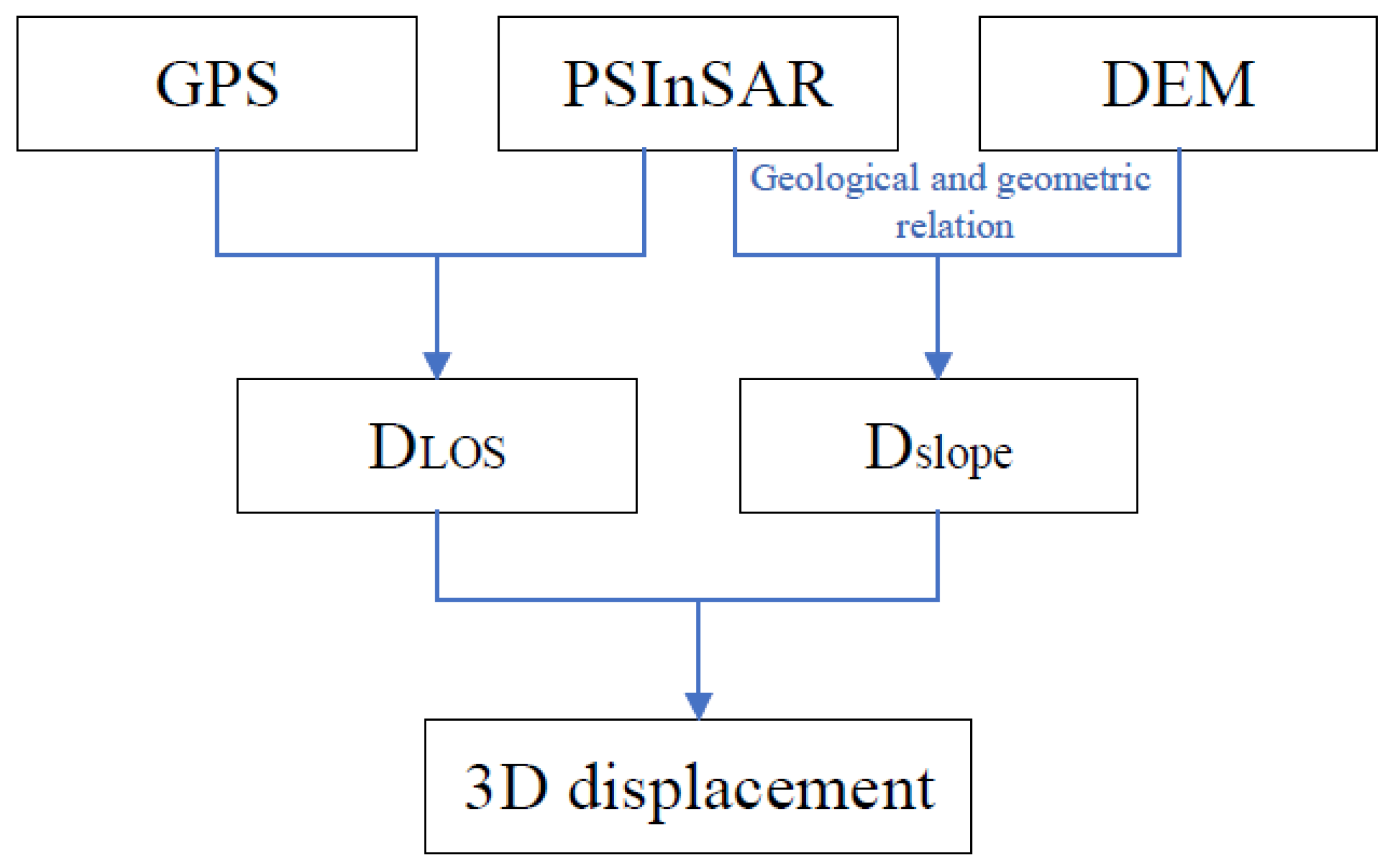
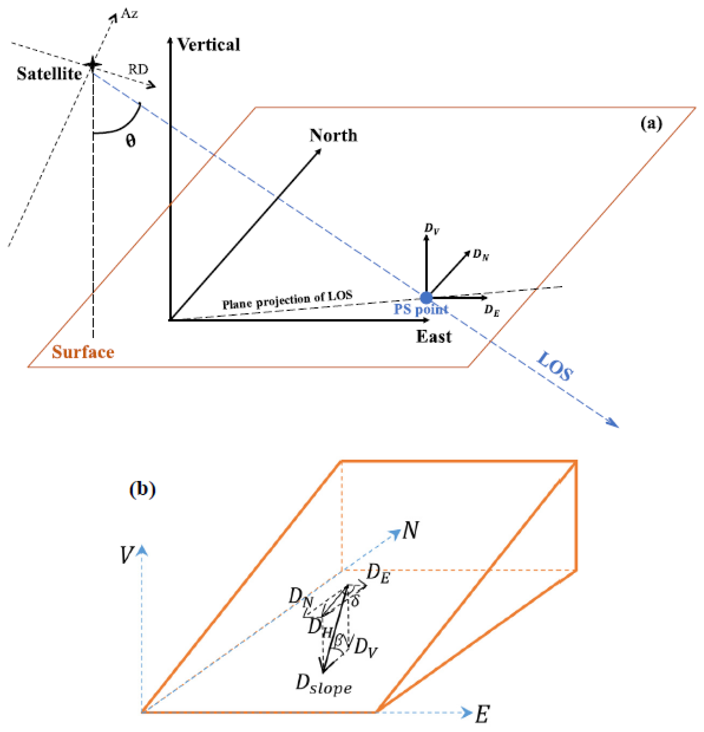
2.2. Algorithm for Calculating 3D Displacement

The ground deformation of PS points is a component parallel to the LOS. However, 1D deformation ($D_{LOS}$) cannot fully represent the real movement. Based on the relationship between the ground geometry and satellite LOS, as shown in Figure 3a, the $D_{LOS}$ can be divided into the north ($D_N$), east ($D_E$), and vertical ($D_V$) directions, which can be expressed as

$$D_{LOS}=(\sin \theta \cos \phi -\sin \theta \sin \phi +\cos \theta )\left[\begin{array}{c}{D}_N\\ D_E\\ D_V\end{array}\right]$$

(4)

where $\theta$ is the incidence angle of the satellite; $\phi =\alpha -\frac{3}{2}\pi$, where $\alpha$ is the azimuth angle of the satellite orbit, clockwise from the north. Equation (5) shows different directions with different weights for $D_{LOS}$. The movement of the landslide is mainly reflected in $D_V$, and the horizontal displacement $D_H$ is the resulting displacement that includes $D_N$ and $D_E$ at the surface. This means that the InSAR technique has high sensitivity for $D_V$ and low sensitivity for $D_H$. The horizontal component of motion is nearly perpendicular to the LOS projection from the general direction of the slope in the landslide area [34,35,36].

The slope deformation ($D_{slope}$) is an along-slope vector that describes the most probable direction of real movement associated with potential slope failure [37,38,39]; from Figure 3b, the formula is as follows:

$$\left\{\begin{array}{c}{D}_N={-D}_{slope}\cos \beta \cos \delta \\ D_E=D_{slope}\cos \beta \sin \delta \\ D_V={-D}_{slope}\sin \beta \end{array}\right.$$

(5)

where $\beta$ is the slope angle, and $\delta$ is the aspect of the slope. When $D_{slope}$ is positive, it indicates uphill movement, while a negative value indicates downhill movement. Moreover, only slope angles of $\beta >5°$ are projected in this study, because it is rare for a landslide to occur when the slope is less than $5°$ [40].

By substituting Equation (5) into Equation (4), $D_{LOS}$ can be expressed using Equation (6):

$$D_{LOS}=\sin \theta \cos \phi \left({-D}_{slope}\cos \beta \cos \delta \right)-\sin \theta \sin \phi \left(D_{slope}\cos \beta \sin \delta \right)+\cos \theta \left({-D}_{slope}\sin \beta \right)$$

(6)

Here, $D_{LOS}$ can be easily obtained using the 3D displacement components $D_N, { D}_E, \mathrm{and} D_V$. However, the 3D displacements could not be derived from $D_{LOS}$ without additional data support. Based on the geometric relationship described in Figure 3b, $D_{slope}$ can be written as

$$D_{slope}=-\frac{D_{LOS}}{\sin \theta \cos \phi \cos \beta \cos \delta +\sin \theta \sin \phi \cos \beta \sin \delta +\cos \theta \sin \beta }$$

(7)

Thus, $D_{slope}$ can be calculated using Equation (7). By substituting known $D_{slope}$ values into Equation (5), the unknown 3D displacement vectors ($D_N, D_E, D_V$) can be transformed as follows:

$$\left[\begin{array}{c}{D}_N\\ D_E\\ D_V\end{array}\right]=B·D_{LOS}$$

(8)

$$B=\left[\begin{array}{c}\frac{\cos \beta \cos \delta }{\sin \theta \cos \phi \cos \beta \cos \delta +\sin \theta \sin \phi \cos \beta \sin \delta +\cos \theta \sin \beta }\\ -\frac{\cos \beta \sin \delta }{\sin \theta \cos \phi \cos \beta \cos \delta +\sin \theta \sin \phi \cos \beta \sin \delta +\cos \theta \sin \beta }\\ \frac{\sin \beta }{\sin \theta \cos \phi \cos \beta \cos \delta +\sin \theta \sin \phi \cos \beta \sin \delta +\cos \theta \sin \beta }\end{array}\right]$$

From Equation (8), the 3D displacement can be easily calculated based on the satellite and geological parameters $\theta , \phi , \beta , \mathrm{and} \delta$. $D_{LOS}$ can be obtained from PSInSAR as described in Section 2.1. The proposed method can then be used to obtain accurate 3D displacements.

3. Experiment and Processing

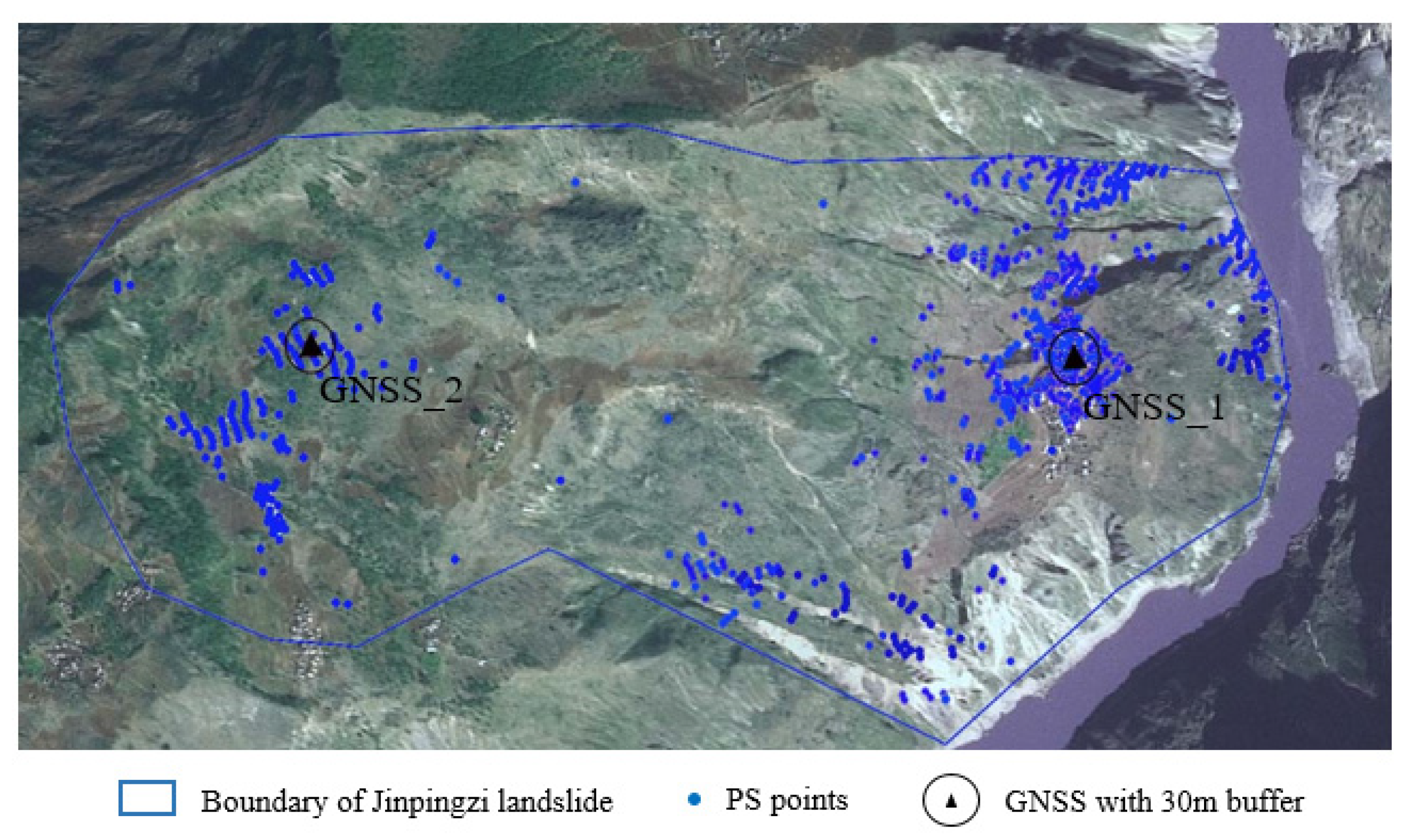
3.1. Study Area

The study area, covering $20 \mathrm{k}\mathrm{m}\times 20 \mathrm{k}\mathrm{m}$, is located in southwest China at the junction of the Yunnan and Sichuan Provinces. The Jinsha River is one of the largest tributaries of the upper Yantze River, which crosses the center of the study area from west to east (Figure 4). Tectonic uplift movement since the Quaternary has resulted in a very narrow and deep river valley. The Wudongde hydropower station is located in the middle of the study area and is one of the largest hydropower stations in China. The Wudongde area is also divided by several faults. Although none of these faults are currently active, there are several active slow-moving landslides near the station area, such as the Jinpingzi and Dashicheng landslides, as shown by the red line in Figure 4. These separate the Wudongde area into several subareas. Thus, it is necessary to monitor the surface deformation over the entire area [41].

The geological structure of this area was studied using field surveys and geotechnical investigations. The elevation ranges from 756 to 3133 m. The geological conditions in this area are complex, with several faults and cracks, as shown in Figure 4. The blue lines represent the river system, and the red lines are fault locations. There are several faults across the middle of the study area. Under the effect of tectonic stress by horizontal compression between the Indian Plate and the Eurasian Plate, the faults are well developed. Moreover, the geological environment is greatly influenced by rainfall and by the water level of the dam (the black circle in Figure 4). The terrain is very undulating in this area; according to the research results by Huang [42], the slope angle of the landslides ranges from 30° to 60°, and the aspect angle ranges from 67.5° to 247.5°. The annual rainfall is 500–900 mm, and the rainy season lasts from June to September. The terrain is a bilayer structure consisting of shale in the superstructure and limestone in the understructure. Precipitation in the rainy season accounts for more than 90% of the annual rainfall. Rock debris deposits were observed on both sides of the river bands. These conditions provide the possibility of landslides.

Jinpingzi landslide is an active landslide located on the right side of Jinsha River. The sliding started in 2005, and the average annual velocity is about 7 to 12 cm/year [43]. The scale is about 3 km long and 1.5 km wide, and it is only 0.9 to 2.5 km downstream from Wudongde hydropower station. The volume of the sliding mass is more than $27\times {10}^6 {\mathrm{m}}^3$ [44]. The deposits in the toe of the landslide have contributed to changing the water level of Jinsha River. Similar dolomite rock debris deposits are found on both sides of the river.

3.2. Dataset

The available radar data consist of 30 SAR images acquired by the Sentinel-1 satellite in the C-band with a descending orbit. The revisit duration was 12 days. The coverage area was approximately 400 km², and the resolution was 5 m × 22 m. The polarization was single VV. The incidence angle was 40.7°, and the azimuth angle was 281.5°. The acquisition period ranged from August 2021 to August 2022. The reference DEM was the ASTGTM2 DEM with a resolution of 30 m [45], which was used to remove topographic phases. The GNSS data consisted of 29 points; the distribution of the GNSS stations is shown in Figure 4, denoted by black triangles. The GNSS stations were sparsely distributed on both sides of Jinsha River. The GNSS data are available from 2005 and established using multi-base station network RTK technology provided by the Yangtze River Survey, Planning, Design and Research Institute. The GNSS revisit time is the same as that for the Sentinel-1 satellite.

3.3. GNSS as Constraining Data in PSInSAR Processing

SARScape 5.2 software was used to process the SAR data. Following the traditional PSInSAR process, which includes interferometry, flattening, filtering, and differential interferometry, 29 interferograms were obtained. To solve the lack of external constraint points in certain areas, GNSS stations were added to the PS network. The phase difference was extracted at each GNSS station, with the nearest PS point used as the reference. Topographic component estimation with absolute height information was obtained from the GNSS receivers. Phase unwrapping was performed using the LAMDBA method to obtain the deformation parameters. After temporal and spatial unwrapping, the GNSS stations as constraining data were used to adjust the PS–GNSS Delaunay triangular network, and the length and deformation information of 29 interferograms without topographic phases were acquired in time series. Finally, the deformation parameter ($D_{LOS}$) and height corrections were obtained for each PS point using Equation (3). $V_{LOS}$ can be calculated from $D_{LOS}$ in time series that combine the horizontal direction and vertical direction.

Figure 5a,b show the $V_{LOS}$ map of PS points without and with GNSS as the constraint, respectively. There are 18,612 and 19,354 points in Figure 5a and Figure 5b, respectively. The negative values in red color show soil movements away from the satellite, while the positive values show movement towards the satellite. In Figure 5a, the subsidence velocity is primarily above 15 mm/year and above 34 mm/y near the Jinsha River. Although the filtering method in PS processing can reduce the atmospheric delay and noise phases, a residual phase still exists. It is also evident that there are points distributed in the river area (considered incorrect points). Amplitude information was considered to eliminate these incorrect points, and a Delaunay triangle with GNSS points as the constraining data was used to revise the phase information. The PS points in the river were discarded in Figure 5b; the color changes are more continuous and have fewer catastrophe points. The deformation trends are similar, but the maximum value in Figure 5a is clearly greater than that in Figure 5b. Comparing the accuracy of PSInSAR with and without GNSS, as shown in Figure 6a,b, the most frequent root-mean-square error (RMSE) values of $v_{LOS}$ were 5 and 10 mm/year, respectively.

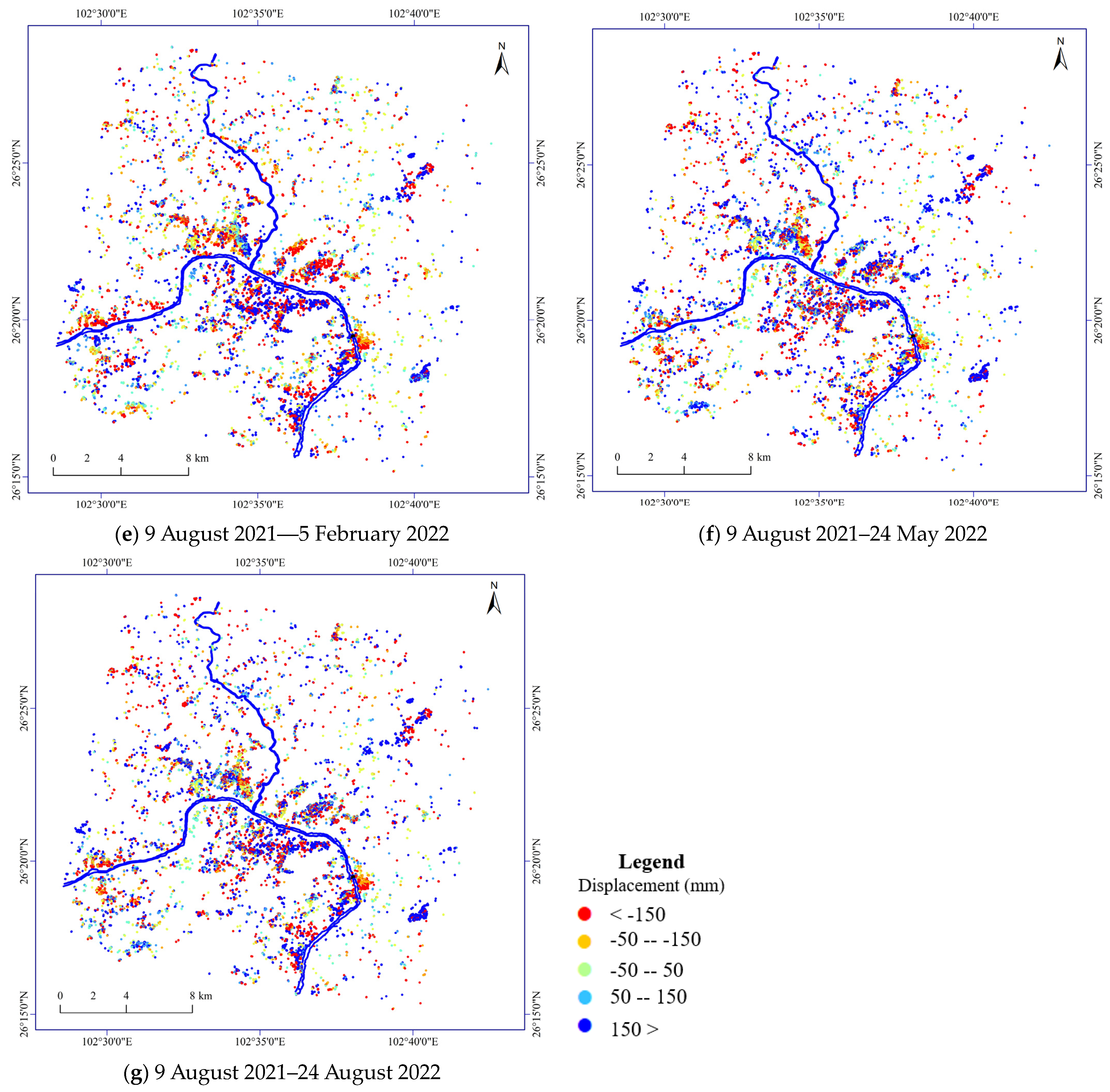
3.4. Three-Dimensional Displacement of Wudongde Area

From the monitoring results for $D_{LOS}$ in Section 3.3, slope and aspect maps were extracted from the DEM and used to calculate $D_{slope}$ using Equation (7), as shown in Figure 7a and Figure 7b, respectively. In Equation (7), the incidence angle $\mathsf{\theta }$ was 40.39°, and the azimuth angle $\phi$ was −78.53°. The $D_{LOS}$ values were transformed into the vertical ($D_V$), east ($D_E$), and north ($D_N$) directions of 3D deformation in the time series. Positive values represent upward, eastward, and northward movements.

Figure 8, Figure 9 and Figure 10 show the vertical (D_V), east (D_E), and north (D_N) deformation maps in the time series. The figures show the deformation from August 2021 to August 2022. The maximum displacements measured approximately 11.5, 25.3, and 20.5 cm in the vertical (D_V), east (D_E), and north (D_N) directions, respectively. Therefore, the vertical direction was not the main direction of sliding. As shown in Figure 8a–f, the displacement increased gradually in the time series, particularly after the rainy season in September, and the displacement increased significantly. At the toe of the slide, the displacement on both sides of the Jinsha River was uplifted because the elevation on both sides of the river was low. Thus, the sliding direction was towards the river.

With the accumulation of landslide bodies, the vertical displacement had a positive value (blue). At the crown of the slide, the displacement exhibits a negative value (orange or red) in Figure 8d–f. In the east (D_E) and north (D_N) directions, the statistical results show that cumulative displacement in the east and north directions reached 10.2 cm and 8.1 cm before the rainy season (June), and the maximum displacement rate increased after the rainy season in September. From Figure 9a–f and Figure 10a–f, the time-series displacement of the Wudongde area in the east and north directions was extracted using the proposed method. The main horizontal displacement direction of the landslides was D_E, followed by D_N.

3.5. Results

According to the results above, GNSS stations can be used as constraint points to obtain more accurate D_LOS values, as shown in Figure 5a. This method can help reduce the outliers in PSInSAR monitoring results, reduce spatial incoherence, and improve monitoring accuracy. Based on the improved D_LOS values, D_slope can be calculated from the slope and aspect. Then, the 3D displacement of the landslide can be calculated from the geometric relationship between D_slope and D_LOS according to Equation (8). The results of 3D displacement in the study area in time series are shown in Figure 8, Figure 9 and Figure 10; the maximum values of D_V, D_N, and D_E are 11.5, 25.3, and 20.5 cm, respectively.

In order to validate the attributes of the time-series displacement acquired through the suggested approach over the course of the observation period in various regions, two sampling points were selected from the crown and toe of Jinpingzi [44], as depicted in Figure 11. The improved PSInSAR technique was employed to observe the three-dimensional displacements within a 30 m radius surrounding the GNSS points.

As illustrated in Figure 12, the monitoring outcomes obtained from these two methodologies exhibited a high level of concordance in all three directions. The D_V, D_N, and D_E values represent 3D displacement calculated by the proposed method, and D_GV, D_GN, and D_GE represent the monitoring results from GNSS stations. The average daily rainfall is 0.3 mm/d in the study area. The 3D displacement of the improved PSInSAR increased significantly after the rainy season, whereas the GNSS stations’ monitored displacement showed a consistent increase. According to the monitoring results, the displacement increased at the next visiting time after the rainy season. From Figure 12, compared with the 3D displacement from the GNSS, the displacement monitored by means of GNSS and InSAR showed the same change trend, increasing significantly at the same time in October. Additionally, the root-mean-square errors (RMSEs) of the D_V, D_N, and D_E values monitored using InSAR and GNSS were ±2 mm, ±2.8 mm, and ±2.6 mm, respectively, indicating good consistency and high precision.

4. Discussion

In this study, a new method for 3D displacement was proposed based on integrated PSInSAR and GNSS. This method has several advantages: Mobile GNSS points can be easily installed in areas without stable points and can be considered as constraining data for the spatial unwrapping of the PS network, removing the redundancy phase of the PS points and making the solutions more stable. The use of GNSS points can avoid the uncertainty of choosing reference points during PS processing. Moreover, this method can be used to calculate the 3D displacement vector directions based on the slope deformation using the combined revised PSInSAR LOS observations.

Though many studies have focused on 3D displacement calculated by InSAR, the normal case to calculate the 3D displacement is to use different sensors of InSAR or different viewing geometries [46,47]. Other observations, like GNSS data and Corner Reflectors (CR) points, can be merged with InSAR LOS measurements to resolve the 3D displacement vectors [48,49]. However, these methods neglect the influence of topographical conditions: Firstly, topographical factors may cause geometric distortions in SAR acquisitions. Additionally, the sliding of a landslide is related to its slope [50]. Therefore, the topographical conditions must be considered in 3D displacement calculations.

The results of the 3D displacement in time series, presented in Figure 8, Figure 9 and Figure 10, reveal the deformation characteristics of a landslide through PSInSAR observations. The Jinpingzi landslide was used to illustrate the deformation characteristics of a landslide in 3D. The thickness of the sliding surface gradually increases in the toe of slide from west to east, accompanied by a gradual increase in the sliding force component caused by gravity. From Figure 4, Figure 9, Figure 10 and Figure 12, it is clear that D_E is larger than D_N, which is related to geological conditions and faults. From the slope map in Figure 7a, the slope in the eastern direction is steeper than that in the northern direction, and the Jinsha River is located east of the landslide. Moreover, several faults passing through the landslide area increased the deformation, as shown in Figure 4.

One of the limitations is the number of GNSS points. In the first step of the PS–GNSS network, there is a high requirement on the number of GNSS points: the more points used, the higher the precision. Another limitation is that surface-parallel flow was not assumed based on the 3D surface deformation. A fault model can be used to aid in the assumption of the sliding surface [51,52]. Meanwhile, rainfall is one of the main factors affecting landslides in this area, but the reservoir water level is another major factor. The rising water level, combined with the rainfall level, accelerates the movement of landslides. It is necessary to consider the influence of changes in the reservoir water level for further research and assume that shear zones are an effective indicator for landslide observation [53,54,55,56].

5. Conclusions

Based on traditional geological engineering investigations, a new method for extracting 3D displacement was proposed by integrating PSInSAR and GNSS points. First, the algorithm uses the subsidence deformation calculated at the GNSS points as constraining data for the PS net in the study area, before estimating the deformation and height phase in the PS network using parametric adjustment. A comparison of the results with and without GNSS points as constraining data showed that the deformation value with GNSS points as a constraint was smaller than that without GNSS points. Second, geological conditions with aspect and slope were used to calculate the 3D displacement using PSInSAR observations. The millimeter-level 3D deformation rate field and time-series displacement from August 2021 to August 2022 were reconstructed and compared with the vertical displacement obtained by the GNSS to verify their reliability. Finally, the deformation mechanism of the Jinpingzi landslide was analyzed using the 3D displacement characteristics. The main conclusions of this study are as follows:

• The accuracy of the deformation rate improved from 10 to 5 mm/year after incorporating PSInSAR with GNSS as the constraining data. The PS–GNSS network can help remove residual phase and height corrections in spatiotemporal unwrapping.
• Geological conditions were used to calculate the 3D displacement. Based on the relationship between InSAR geometric features and geological conditions, $D_{slope}$ was proposed to calculate the 3D displacement using PSInSAR observations. The $D_{LOS}$ value was converted into vertical, east, and north displacements with maximum values of 11.5, 25.3, and 20.5 cm over the study period, respectively. The vertical direction was not the main sliding direction in the Wudongde area, and the north and east displacements were 2–3 times larger than that in the vertical direction.
• The response time of the 3D displacement to rainfall exhibited hysteresis. Vertical displacement was the earliest response, occurring half a month after the rainfall season. The highest average deformation rate occurred in mid-October.
• When compared to the vertical displacement from the GNSS in the Jinpingzi landslide, the calculated 3D displacement from PSInSAR was proven to have high accuracy, and the deformation mechanism of the Jinpingzi landslide was analyzed. The sliding started at the toe of the slide and extended to the crown of the slide.

References

1. Refice, A.; Spalluto, L.; Bovenga, F.; Fiore, A.; Miccoli, M.N.; Muzzicato, P.; Nitti, D.O.; Nutricato, R.; Pasquariello, G. Integration of persistent scatterer interferometry and ground data for landslide monitoring: The Pianello landslide (Bovino, Southern Italy). Landslides 2019, 16, 447–468. [Google Scholar] [CrossRef]
2. Jo, M.J.; Jung, H.S.; Won, J.S. Detecting the Source Location of Recent Summit Inflation via Three-Dimensional InSAR Observation of Kilauea Volcano. Remote Sens. 2015, 7, 14386–14402. [Google Scholar] [CrossRef]
3. Hu, J.; Shi, J.W.; Liu, J.H.; Zheng, W.J.; Zhu, K. Calculating Co-Seismic Three-Dimensional Displacements from InSAR Observations with the Dislocation Model-Based Displacement Direction Constraint: Application to the 23 July 2020 Mw6.3 Nima Earthquake, China. Remote Sens. 2022, 14, 4481. [Google Scholar] [CrossRef]
4. Hamdi, L.; Defaflia, N.; Merghadi, A.; Fehdi, C.; Yunus, A.P.; Dou, J.; Pham, Q.B.; Abdo, H.G.; Almohamad, H.; Al-Mutiry, M. Ground Surface Deformation Analysis Integrating InSAR and GNSS Data in the Karstic Terrain of Cheria Basin, Algeria. Remote Sens. 2023, 15, 1486. [Google Scholar] [CrossRef]
5. Zhao, Y.; Wang, H.; Zhang, Q.; Zhang, D.; Xie, Y.; Yang, J. A study of landslide deformation fields with a digital correlation method. Nat. Hazards 2017, 89, 859–869. [Google Scholar] [CrossRef]
6. Yin, Y.; Liu, X.; Zhao, C.; Tomás, R.; Zhang, Q.; Lu, Z.; Li, B. Multi-dimensional and long-term time series monitoring and early warning of landslide hazard with improved cross-platform SAR offset tracking method. Sci. China Technol. Sci. 2022, 65, 1891–1912. [Google Scholar] [CrossRef]
7. Lei, K.C.; Ma, F.; Chen, B.; Luo, Y.; Cui, W.; Zhou, Y.; Liu, H.; Sha, T. Three-Dimensional Surface Deformation Characteristics Based on Time Series InSAR and GNSS Technologies in Beijing, China. Remote Sens. 2021, 13, 3964. [Google Scholar] [CrossRef]
8. Liu, Y.H.; Wang, G.Q.; Yu, X.; Wang, K. Sentinel-1 InSAR and GNSS-Integrated Long-Term and Seasonal Subsidence Monitoring in Houston, Texas, USA. Remote Sens. 2022, 14, 6184. [Google Scholar] [CrossRef]
9. Ma, Y.Y.; Li, F.; Wang, Z.M.; Zou, X.Q.; An, J.C.; Li, B. Landslide Assessment and Monitoring along the Jinsha River, Southwest China, by Combining InSAR and GNSS Techniques. J. Sens. 2022, 2022, 9572937. [Google Scholar] [CrossRef]
10. Ferretti, A.; Prati, C.; Rocca, F. Permanent Scatterers in SAR Interferomerty. IEEE Trans. Geosci. Remote Sens. 2001, 39, 8–20. [Google Scholar] [CrossRef]
11. Berardino, P.; Gianfranco, F.; Riccardo, L.; Eugenio, S. A new algorithm for surface deformation monitoring based on small baseline differential SAR interferograms. IEEE Trans. Geosci. Remote Sens. 2002, 40, 2375–2383. [Google Scholar] [CrossRef]
12. Komac, M.; Holley, R.; Mahapatra, P.; van der Marel, H.; Bavec, M. Coupling of GNSS/GNSS and radar interferometric data for a 3D surface displacement monitoring of landslides. Landslides 2015, 12, 241–257. [Google Scholar] [CrossRef]
13. Song, X.G.; Jiang, Y.; Shan, X.J.; Qu, C.Y. Deriving 3D coseismic deformation field by combining GNSS and InSAR data based on the elastic dislocation model. Int. J. Appl. Earth Obs. Geoinf. 2017, 57, 104–112. [Google Scholar] [CrossRef]
14. Chen, M.K.; Xu, G.Y.; Zhang, T.X.; Xie, X.W.; Chen, Z.P. A novel method for inverting coseismic 3D surface deformation using InSAR considering the weight influence of the spatial distribution of GNSS points. Adv. Space Res. 2024, 73, 585–596. [Google Scholar] [CrossRef]
15. Zhang, Z.W.; Wang, X.L.; Wu, Y.D.; Zhao, Z.P.; Yang, E. Applied Research on InSAR and GNSS Data Fusion in Deformation Monitoring. Sci. Program. 2021, 2021, 3888975. [Google Scholar]
16. Chen, Q.A.; Liu, G.X.; Ding, X.L.; Hu, J.C.; Yuan, L.G.; Zhong, P.; Omura, M. Tight integration of GNSS observations and persistent scatterer InSAR for detecting vertical ground motion in Hong Kong. Int. J. Appl. Earth Obs. 2010, 12, 477–486. [Google Scholar]
17. Shi, X.G.; Zhang, L.; Zhou, C.; Li, M.H.; Liao, M.S. Retrieval of time series three-dimensional landslide surface displacements from multi-angular SAR observations. Landslides 2018, 15, 1015–1027. [Google Scholar] [CrossRef]
18. Xiong, L.Y.; Xu, C.J.; Liu, Y.; Wen, Y.M.; Fang, J. 3D Displacement Field of Wenchuan Earthquake Based on Iterative Least Squares for Virtual Observation and GNSS/InSAR Observations. Remote Sens. 2020, 12, 977. [Google Scholar] [CrossRef]
19. Ren, K.Y.; Yao, X.; Li, R.J.; Zhou, Z.K.; Yao, C.C.; Jiang, S. 3D displacement and deformation mechanism of deep-seated gravitational slope deformation revealed by InSAR: A case study in Wudongde Reservoir, Jinsha River. Landslides 2022, 19, 2159–2175. [Google Scholar] [CrossRef]
20. Hu, J.; Li, Z.W.; Ding, X.L.; Zhu, J.J.; Zhang, L.; Sun, Q. 3D coseismic Displacement of 2010 Darfield, New Zealand earthquake estimated from multi-aperture InSAR and D-InSAR measurements. J. Geod. 2012, 86, 1029–1041. [Google Scholar] [CrossRef]
21. Dematteis, N.; Wrzesniak, A.; Allasia, P.; Bertolo, D.; Giordan, D. Integration of robotic total station and digital image correlation to assess the three-dimensional surface kinematics of a landslide. Eng. Geol. 2022, 303, 106655. [Google Scholar] [CrossRef]
22. Rodriguez, J.; Deane, E.; Hendry, M.T.; Macciotta, R.; Evans, T.; Gräpel, C.; Skirrow, R. Practical evaluation of single-frequency dGNSS for monitoring slow-moving landslides. Landslides 2021, 18, 3671–3684. [Google Scholar]
23. Corsini, A.; Bonacini, F.; Mulas, M.; Ronchetti, F.; Monni, A.; Pignone, S.; Primerano, S.; Bertolini, G.; Caputo, G.; Truffelli, G.; et al. A portable continuous GPS array used as rapid deployment monitoring system during landslide emergencies in Emilia Romagna. Rend. Online Soc. Geol. Ital. 2015, 35, 89–91. [Google Scholar] [CrossRef]
24. Simons, W.; Broerse, T.; Shen, L.; Kleptsova, O.; Nijholt, N.; Hooper, A.; Pietrzak, J.; Morishita, Y.; Naeije, M.; Lhermitte, S.; et al. A Tsunami Generated by a Strike-Slip Event: Constraints From GPS and SAR Data on the 2018 Palu Earthquake. J. Geophys. Res. Solid Earth 2022, 127, e2022JB024191. [Google Scholar] [CrossRef]
25. Zambanini, C.; Reinprecht, V.; Kieffer, D.S. InSARTrac Field Tests-Combining Computer Vision and Terrestrial InSAR for 3D Displacement Monitoring. Remote Sens. 2023, 15, 2031. [Google Scholar] [CrossRef]
26. Hu, J.; Li, Z.W.; Ding, X.L.; Zhu, J.J.; Zhang, L.; Sun, Q. Resolving three-dimensional surface displacements from InSAR measurements: A review. Earth-Sci. Rev. 2014, 133, 1–17. [Google Scholar] [CrossRef]
27. Bickel, V.T.; Manconi, A.; Amann, F. Quantitative Assessment of Digital Image Correlation Methods to Detect and Monitor Surface Displacements of Large Slope Instabilities. Remote Sens. 2018, 10, 865. [Google Scholar] [CrossRef]
28. Xu, K.; Gan, W.; Wu, J.; Hou, Z. A robust method for 3D surface displacement fields combining GNSS and single-orbit InSAR measurements with directional constraint from elasticity model. GPS Solut. 2022, 26, 46. [Google Scholar] [CrossRef]
29. Ciampalini, A.; Raspini, F.; Lagomarsino, D.; Catani, F.; Casagli, N. Landslide susceptibility map refinement using PSInSAR data. Remote Sens. Environ. 2016, 184, 302–315. [Google Scholar] [CrossRef]
30. Yuan, M.Z.; Li, M.; Liu, H.; Lv, P.Y.; Li, B.; Zheng, W.B. Subsidence Monitoring Base on SBAS-InSAR and Slope Stability Analysis Method for Damage Analysis in Mountainous Mining Subsidence Regions. Remote Sens. 2021, 13, 3107. [Google Scholar] [CrossRef]
31. Yin, Y.P.; Zheng, W.M.; Liu, Y.P.; Zhang, J.L.; Li, X.C. Integration of GPS with InSAR to monitoring of the Jiaju landslide in Sichuan, China. Landslides 2010, 7, 359–365. [Google Scholar] [CrossRef]
32. Teshebaeva, K.; Roessner, S.; Echtler, H.; Motagh, M.; Wetzel, H.U.; Molodbekov, B. ALOS/PALSAR InSAR Time-Series Analysis for Detecting Very Slow-Moving Landslides in Southern Kyrgyzstan. Remote Sens. 2015, 7, 8973–8994. [Google Scholar] [CrossRef]
33. Xing, X.M.; Zhu, J.J.; Wang, Y.Z.; Yang, Y.F. Time series ground subsidence inversion in mining area based on CRInSAR and PSInSAR integration. J. Cent. South Univ. 2013, 20, 2498–2509. [Google Scholar] [CrossRef]
34. Dai, Z.L.; Huang, Y.; Cheng, H.L.; Xu, Q. 3D numerical modeling using smoothed particle hydrodynamics of flow-like landslide propagation triggered by the 2008 Wenchuan earthquake. Eng. Geol. 2014, 180, 21–33. [Google Scholar] [CrossRef]
35. Franz, M.; Carrea, D.; Abellan, A.; Derron, M.H.; Jaboyedoff, M. Use of targets to track 3D displacements in highly vegetated areas affected by landslides. Landslides 2016, 13, 821–831. [Google Scholar] [CrossRef]
36. Gojcic, Z.; Schmid, L.; Wieser, A. Dense 3D displacement vector fields for point cloud-based landslide monitoring. Landslides 2021, 18, 3821–3832. [Google Scholar] [CrossRef]
37. Salih, W.H.M.; Soons, J.A.M.; Dirckx, J.J.J. 3D displacement of the middle ear ossicles in the quasi-static pressure regime using new X-ray stereoscopy technique. Hear. Res. 2016, 340, 60–68. [Google Scholar] [CrossRef]
38. Donati, D.; Rabus, B.; Engelbrecht, J.; Stead, D.; Clague, J.; Francioni, M. A Robust SAR Speckle Tracking Workflow for Measuring and Interpreting the 3D Surface Displacement of Landslides. Remote Sens. 2021, 13, 3048. [Google Scholar] [CrossRef]
39. Eriksen, H.O.; Bergh, S.G.; Larsen, Y.; Skrede, I.; Kristensen, L.; Lauknes, T.R.; Blikra, L.H.; Kierulf, H.P. Relating 3D surface displacement from satellite- and ground-based InSAR to structures and geomorphology of the Jettan rockslide, northern Norway. Nor. J. Geol. 2017, 97, 283–303. [Google Scholar] [CrossRef]
40. Xiong, L.Y.; Xu, C.J.; Liu, Y.; Zhao, Y.W.; Geng, J.H.; Francisco, O.C. Three-dimensional displacement field of the 2010 Mw 8.8 Maule earthquake from GNSS and InSAR data with the improved ESISTEM-VCE method. Front. Earth Sci. 2022, 10, 970493. [Google Scholar] [CrossRef]
41. Xie, M.W.; Huang, J.X.; Wang, L.W.; Huang, J.H.; Wang, Z.F. Early landslide detection based on D-InSAR technique at the Wudongde hydropower reservoir. Environ. Earth Sci. 2016, 75, 717. [Google Scholar] [CrossRef]
42. Huang, J.X.; Xie, M.W.; Atkinson, P.M. Dynamic susceptibility mapping of slow-moving landslides using PSInSAR. Int. J. Remote Sens. 2020, 41, 7509–7529. [Google Scholar]
43. Jiang, S.; Wang, Y.F.; Tang, C.; Pan, H.; Wang, K. Preliminary study of the creep mechanism of Jinpingzi zone II slow moving landslide in lower reaches of Jinsha River. J. Eng. Geol. 2017, 25, 1547–1556. [Google Scholar]
44. Jiang, S.; Wang, Y.F.; Tang, C.; Liu, K. Long-term kinematics and mechanism of a deep-seated slow-moving debris slide near Wudongde hydropower station in Southwest China. J. Mt. Sci. 2018, 15, 364–379. [Google Scholar] [CrossRef]
45. Ettazarini, S. GIS-based land suitability assessment for check dam site location, using topography and drainage information: A case study from Morocco. Environ. Earth Sci. 2021, 80, 567. [Google Scholar] [CrossRef]
46. Highland, L.; Bobrowsky, P.T. The Landslide Handbook—A Guide to Understanding Landslides; US Geological Survey: Reston, VA, USA, 2008; pp. 1–47.
47. Fey, C.; Rutzinger, M.; Wichmann, V.; Prager, C.; Bremer, M.; Zangerl, C. Deriving 3D displacement vectors from multi-temporal airborne laser scanning data for landslide activity analyses. GISci. Remote Sens. 2015, 52, 437–461. [Google Scholar] [CrossRef]
48. Guglielmino, F.; Anzidei, M.; Briole, P.; Elias, P.; Puglisi, G. 3D displacement maps of the 2009 L’Aquila earthquake (Italy) by applying the SISTEM method to GNSS and DInSAR data. Terra Nova 2013, 25, 79–85. [Google Scholar] [CrossRef]
49. Bovenga, F.; Pasquariello, G.; Pellicani, R.; Refice, A.; Spilotro, G. Landslide monitoring for risk mitigation by using corner reflector and satellite SAR interferometry: The large landslide of Carlantino (Italy). CATENA 2017, 151, 49–62. [Google Scholar] [CrossRef]
50. Mazzanti, P.; Caporossi, P.; Muzi, R. Sliding Time Master Digital Image Correlation Analyses of CubeSat Images for landslide Monitoring: The Rattlesnake Hills Landslide (USA). Remote Sens. 2020, 12, 592. [Google Scholar] [CrossRef]
51. Budimir, M.; Atkinson, P.M.; Lewis, H. A systematic review of landslide probability mapping using logistic regression. Landslides 2015, 12, 419–436. [Google Scholar] [CrossRef]
52. Huang, Y.T.; Li, W.; Jiang, X. Co-seismic deformation field of the 2020 Nima Tibet Earthquake and fault slip distribution. Bull. Surv. Mapp. 2021, S1, 173–177. [Google Scholar] [CrossRef]
53. Li, K.; Li, Y.; Tapponnier, P.; Xu, X.; Li, D.; He, Z. Joint InSAR and Field Constraints on Faulting During the Mw 6.4, July 23, 2020, Nima/Rongma Earthquake in Central Tibet. J. Geophys. Res. Solid Earth 2021, 126, e2021JB022212. [Google Scholar]
54. Wu, Q.; Liu, Y.X.; Tang, H.M.; Kang, J.T.; Wang, L.Q.; Li, C.D.; Wang, D.; Liu, Z.Q. Experimental study of the influence of wetting and drying cycles on the strength of intact rock samples from a red stratum in the Three Gorges Reservoir area. Eng. Geol. 2023, 314, 107013. [Google Scholar] [CrossRef]
55. Fang, K.; Tang, H.M.; Li, C.D.; Su, X.X.; An, P.J.; Sun, S.X. Centrifuge modelling of landslides and landslide hazard mitigation: A review. Geosci. Front. 2023, 14, 101493. [Google Scholar] [CrossRef]
56. Wang, C.; Wang, H.; Qin, W.; Wei, S.; Tian, H.; Fang, K. Behaviour of pile-anchor reinforced landslides under varying water level, rainfall, and thrust load: Insight from physical modelling. Eng. Geol. 2023, 325, 107293. [Google Scholar] [CrossRef]
Figure 1. Flowchart of the method.
Land 13 00429 g001
Figure 2. PS network with GNSS points.
Land 13 00429 g002
Figure 3. Geometric map of DLOS (a) and Dslope (b).
Land 13 00429 g003
Figure 4. Geographical location of the Wudongde area.
Land 13 00429 g004
Figure 5. Velocity map of the study area with (a) and without GNSS points (b). The blue points represent the uplifted areas, and the red points represent the subsidence areas. The red line represents the Jinpingzi landslide area.
Land 13 00429 g005
Figure 6. RMSE values of velocity with (a) and without GNSS points (b).
Land 13 00429 g006aLand 13 00429 g006b
Figure 7. Slope (a) and aspect maps (b) of the study area.
Land 13 00429 g007aLand 13 00429 g007b
Figure 8. Time series of the vertical displacement (DV) in the study area.
Land 13 00429 g008aLand 13 00429 g008b
Figure 9. Time series of the eastward displacement (DE) in the study area.
Land 13 00429 g009aLand 13 00429 g009b
Figure 10. Time series of the northward displacement (DN) in the study area.
Land 13 00429 g010aLand 13 00429 g010b
Figure 11. PS and GNSS points in Jinpingzi landslide.
Land 13 00429 g011
Figure 12. The 3D time series displacement from PSInSAR and GNSS in Jinpingzi landslide. The DV, DN, and DE values represent 3D displacement calculated by the proposed method, and DGV, DGN, and DGE represent the monitoring results from GNSS stations.
Land 13 00429 g012
Disclaimer/Publisher’s Note: The statements, opinions and data contained in all publications are solely those of the individual author(s) and contributor(s) and not of MDPI and/or the editor(s). MDPI and/or the editor(s) disclaim responsibility for any injury to people or property resulting from any ideas, methods, instructions or products referred to in the content.