Article

Spatio-Temporal Dynamics of Carbon Emissions and Their Influencing Factors at the County Scale: A Case Study of Zhejiang Province, China

1
College of Art and Archaeology, Hangzhou City University, Hangzhou 310015, China
2
Beautiful Hangzhou Environmental Planning and Architectural Design Research Center, Hangzhou City University, Hangzhou 310015, China
3
College of Civil Engineering and Architecture, Zhejiang University, Hangzhou 310058, China
4
Center for Balance Architecture, Zhejiang University, Hangzhou 310058, China
5
Architectural Design and Research Institute of Zhejiang University Co., Ltd., Hangzhou 310058, China
*
Author to whom correspondence should be addressed.
Land 2024, 13(3), 381; https://doi.org/10.3390/land13030381
Submission received: 6 February 2024 / Revised: 10 March 2024 / Accepted: 14 March 2024 / Published: 17 March 2024
(This article belongs to the Special Issue Urban Planning Pathways to Carbon Neutrality)

Abstract

:
Significant carbon emissions, a key contributor to global climate warming, pose risks to ecosystems and human living conditions. It is crucial to monitor the spatial and temporal patterns of carbon emissions at the county level to reach the goals of carbon peak and neutrality. This study examines carbon emissions and economic and social problems data from 89 counties in Zhejiang Province. It employs analytical techniques such as LISA time path, spatio-temporal transition, and standard deviational ellipse to investigate the trends of carbon emissions from 2002 to 2022. Furthermore, it utilizes the GTWR model to evaluate the factors that influence these emissions on a county scale. The findings reveal the following: (1) The LISA time path analysis indicates a pronounced local spatial structure in the distribution of carbon emissions in Zhejiang Province from 2002 to 2022, characterized by increasing stability, notable path dependency, and some degree of spatial integration, albeit with a diminishing trend in overall integration. (2) The LISA spatio-temporal transition analysis indicates significant path dependency or lock-in effects in the county-level spatial clustering of carbon emissions. (3) Over the period 2002–2022, the centroid of carbon emissions in Zhejiang’s counties mainly oscillated between 120°55′15″ E and 120°57′01″ E and between 29°55′52″ N and 29°59′11″ N, with a general northeastward shift forming a “V” pattern. This shift resulted in a stable “northeast–southwest” spatial distribution. (4) Factors such as population size, urbanization rate, and economic development level predominantly accelerate carbon emissions, whereas industrial structure tends to curb them. It is crucial to customize carbon mitigation plans to suit the circumstances of each county. This study provides insight into the spatial and temporal patterns of carbon emissions at the county level in Zhejiang Province. It offers crucial guidance for developing targeted and practical strategies to reduce carbon emissions.

1. Introduction

Several crises, such as water scarcity, food insecurity, and public health emergencies, are being brought on by recent trends in global warming, which have led to a persistent degradation of the ecological environment and a threat to human survival [1,2,3]. The primary cause of global warming is the increase in carbon dioxide emissions. As a result, the world community has focused its efforts on reducing these emissions, encouraging low-carbon, sustainable growth and supporting ecological preservation [4,5,6]. Following a sharp increase in emissions, China overtook the US as the world’s top carbon producer in 2007 [7]. By 2022, China’s carbon emissions had surged to 11.48 billion tons, marking an annual growth rate of 3.7% since 2018 [8]. Predominantly, these emissions stem from fossil fuels, comprising 84.1% of China’s total in 2020 [9]. As a result, China has actively looked for ways to reduce its carbon footprint, set several goals and policies [10,11], and, at the 75th UN General Assembly, declared its intention to achieve carbon neutrality by 2060 and a carbon peak by 2030, reiterating its commitment to a comprehensive green transition [12].
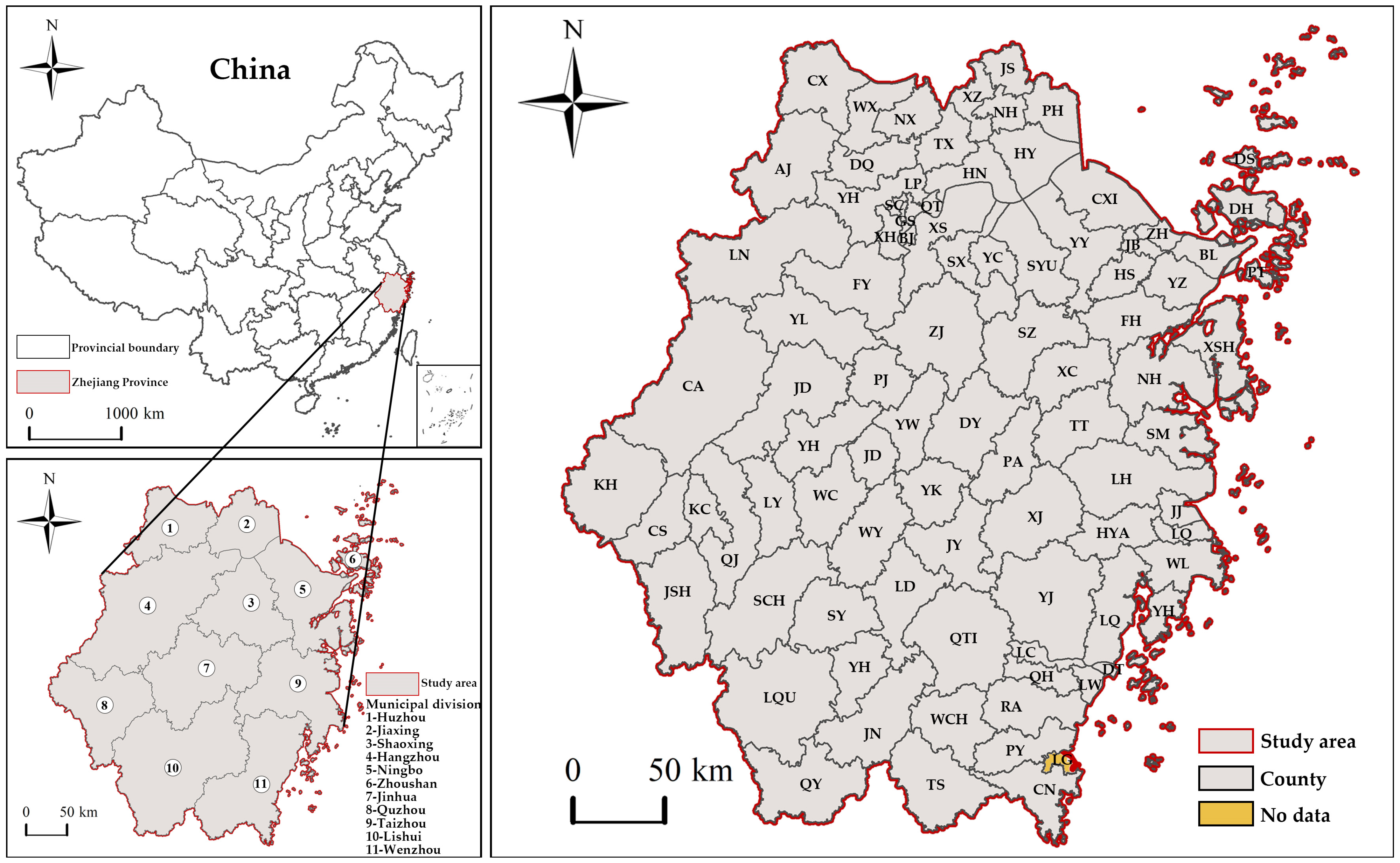
Counties, serving as the core administrative entities and spatial foundations for industrial and economic expansion in China [13], encompass 78% of the nation’s landmass, are home to two-thirds of its population, and contribute approximately 51.8% to China’s GDP [14]. The county-level administrative divisions here include counties (such as Deqing county, Cangnan county, and Panan county), county-level cities (Dongyang City, Cixi City, and Yueqing City), and districts (Wucheng district, Yuhang district, and Haishu district) under city jurisdiction. Notably, they are responsible for over half of the nation’s carbon emissions [15], underscoring the immense potential and urgent need for low-carbon initiatives at this level, which are crucial for China’s carbon neutrality aspirations [16]. Achieving these reduction goals entails national macro-strategic planning and an emphasis on localized carbon emission strategies [17]. Hence, it is crucial to examine county-level carbon emissions thoroughly, accurately chart their spatio-temporal progression, and comprehend the factors that drive them. Acquiring this knowledge is essential for fostering regional cooperation in sustainable growth and improving the scientific accuracy, execution, and efficacy of energy conservation and emissions reduction strategies [15].
Researchers in the modern era have used a wide variety of analytical tools to focus more on the temporal and spatial patterns of carbon emissions. Duman [18] utilized the standard deviational ellipse (SDE). They observed a progressive change in the trajectory of urban carbon emissions in China, transitioning from a “northeast–southwest” to a “northwest–southeast” orientation. Concurrently, the standard deviation ellipse grew, indicating that air pollution and carbon dioxide emissions had expanded in space over time. Liu [19] utilized spatial autocorrelation (SA) to reveal notable geographical variation, self-correlation, and spillover effects associated with urbanization and carbon emissions. Zhang [20] utilized Kernel Density Estimation (KDE) for their study, effectively pinpointing spatial associations between carbon emission patterns and land-use-related emissions. In another investigation, Soares [21] utilized the Gini Index (GI) to analyze the world’s 50 major economies and discovered a strong correlation between economic levels and carbon emissions, revealing that higher economic levels lead to greater carbon emissions. Williams [22] employed the Coefficient of Variation (CV) to analyze carbon emission patterns in the Southern Ocean and discovered that this region significantly contributes to the sequestration of heat and the absorption of anthropogenic carbon. These research works provide essential perspectives on the spatio-temporal patterns of carbon emissions. However, the main focus of these studies has been on the provincial and municipal levels, with significantly less attention paid to the county level. This discrepancy underscores the necessity for more detailed research at a finer scale. Delving into these aspects at a more granular level is crucial for understanding the subtle dynamics of spatial interactions and the specific impacts between neighboring areas. Such an approach can aid in the formulation of more effective and targeted decision-making and planning strategies.
Understanding the factors influencing carbon emissions is vital for advancing carbon reduction and environmental improvement. Scholars frequently employ methods like Spatial Econometric Regression Models (SEMs), Logarithmic Mean Divisia Index (LMDI), Geographically Weighted Regression (GWR), Multiscale Geographically Weighted Regression (MGWR) models, and STIRPAT models in their research. For example, Qu [23] analyzed the spatial response mechanism between carbon emission efficiency and ecosystem services using SEMs, finding that overall ecosystem services are influenced not only by local carbon emission efficiency but also by that of surrounding areas. Quan [24] and González [25], through their analysis with the LMDI model, discovered that in Spain, factors related to per capita output are predominant in the industrial sector, while factors related to carbonization effects play a critical role in the commercial sector. Khodakarami [26] used the GWR model to study how trees capture carbon, absorb CO2, and produce oxygen across different areas and what affects these processes. He found that the carbon-absorbing services of urban green spaces are key to cutting greenhouse gas emissions and supporting sustainable environmental development. Li [27] utilized the MGWR model to investigate the determinants of urban carbon emissions in China. Their findings uncovered geographical variations in the effects of per capita GDP, secondary industry percentage, and population density on carbon emissions. Nosheen [28] used the STIRPAT model to analyze the factors affecting carbon emissions in some Asian countries and found that energy consumption and urbanization contribute to increasing carbon emissions. Although these studies provide valuable insights into the factors affecting carbon emissions, they often focus more on the overall positive and negative impacts during the entire phase, without delving into the temporal and spatial changes of these factors. Thus, there is a need for in-depth research from different temporal and spatial perspectives to clearly observe the changes in the time series of influencing factors and to reveal local factors causing regional disparities. By expanding the research scope to these aspects, it becomes possible to gain a more detailed understanding of the reasons affecting carbon emissions, thereby formulating more targeted and effective mitigation and adaptation strategies.
This article endeavors to clarify the spatial–temporal aspects of carbon emissions at the county scale in Zhejiang Province using ESTDA methods, including LISA time path and LISA spatio-temporal transition, as well as the standard deviational ellipse. The GTWR model is utilized to investigate the factors influencing carbon emissions at this level. This study is innovative in two key respects: Firstly, it adopts a micro-scale approach, analyzing the spatio-temporal attributes of carbon emissions at the county level in Zhejiang Province, marking a shift from static to dynamic research methodologies. Secondly, it leverages the GTWR model’s capacity to account for the spatio-temporal heterogeneity of influencing factors. It enables a more nuanced understanding of these factors on carbon emissions, in contrast to traditional global regression methods. This approach is valuable for policymakers developing targeted carbon reduction strategies. The research objectives were as follows: (1) to collect and examine Zhejiang Province county-level carbon emission data in order to shed light on the spatio-temporal aspects of these emissions; (2) to create and employ a GTWR model for analyzing the factors that affect carbon emissions in different spatial and temporal dimensions within Zhejiang Province; and (3) to integrate the findings from both analyses to formulate viable strategies and recommendations for reducing carbon emissions at the county level.
The remainder of this work is organized in the following manner: Section 2 outlines the data sources and methodologies used in this research. Section 3 explores the spatial and temporal dynamics of carbon emissions, along with their determinants at the county level in Zhejiang Province. Section 4 consolidates the key results, discusses possible approaches and suggestions, recognizes the limitations of this study, and suggests future research avenues and areas of focus.
Based on this research gap, this study aimed to investigate the spatio-temporal patterns of carbon emissions and their influencing factors from a micro-perspective of county scale. Therefore, we proposed two research questions:
RQ1. How do the local development directions and global trajectories of the spatio-temporal pattern of carbon emissions at the county level in Zhejiang Province change?
RQ2. What factors drive the changes in the spatio-temporal pattern of carbon emissions at the county level in Zhejiang Province?
This paper contributes to the literature on carbon emissions in several ways: First, it delves into the county scale, moving beyond the provincial and city scales. Second, it examines the spatio-temporal pattern of carbon emissions at the county level in Zhejiang Province from both local and global dimensions. Third, it explores the factors affecting the spatio-temporal distribution of carbon emissions at the county level in Zhejiang Province and analyzes the spatio-temporal changes of significant influencing factors.

2. Materials and Methods

2.1. Research Framework

Our empirical research framework is illustrated in Figure 1. Firstly, we organized and processed data from the China Emissions Accounts and Datasets (CEAD), Zhejiang Statistical Yearbooks, and some municipal statistical yearbooks for the years 2002–2022, generating both total carbon emission data and data on influencing factors composed of multiple indicators. Secondly, based on the total carbon emissions of each county over the years, we comprehensively elucidated the spatio-temporal evolution of county-level carbon emissions in terms of spatial distribution, regional disparities, and temporal evolution using LISA time path, LISA spatio-temporal transitions, and standard deviation ellipse methods. The analysis of relative length in the LISA time path examined the dynamic nature of local spatial dependence and structure, while the analysis of curvature examined the direction of local spatial dependence, and the analysis of transfer direction assessed the competitive situation between neighboring counties. The LISA spatio-temporal transitions analysis evaluated the transfer of local spatial association types, thereby determining the stability of county-level spatial positions [15]. The analysis of centroid displacement, centroid distribution, and ellipse orientation in the standard deviation ellipse examined the overall spatial distribution and spatio-temporal trend [18]. The former two were analyzed from a local perspective, while the latter was analyzed from a global perspective. Finally, we conducted OLS and GWR analyses to examine and eliminate inappropriate indicators from the total carbon emission and influencing factor data, and then constructed a GTWR model to analyze the positive and negative impacts of key factors on county-level carbon emissions, which are of great significance for government policy formulation and intervention planning [26].

2.2. Research Area

Zhejiang Province is located on the southern bank of the Yangtze River Delta in China’s southeastern coastline region. It extends from 27°02′ to 31°11′ N latitude and 118°01′ to 123°10′ E longitude. Comprising ten cities, Zhejiang Province added one county-level city in the 2021 administrative division adjustment, totaling 90 county-level administrative districts (Figure 2). Although Zhejiang’s area accounts for less than 1.5% of the country’s total, its per capita GDP in 2021 reached RMB 113,900, ranking fifth nationwide, with a gross domestic product amounting to RMB 6.5 trillion [29,30]. Nevertheless, the swift pace of development has brought about a multitude of environmental challenges, among which is the escalation of carbon emissions. As an “Ecological Civilization Demonstration Zone”, the Zhejiang Provincial Government is committed to fostering a low-carbon economy, aiming to mitigate carbon emissions through strategic spatial planning [31]. Over the years, it has implemented policies such as “Implementation Opinions on Supporting Work for Carbon Peak and Carbon Neutrality” and “Zhejiang Province’s 14th Five-Year Plan for Energy Conservation and Emission Reduction.” The province’s efforts in energy conservation and decreasing emissions have been particularly effective, making it a remarkable case for research with significant demonstrative and referential relevance.

2.3. Data Sources

This study selected 90 districts and counties in Zhejiang Province as research subjects. To analyze the spatial and temporal patterns of carbon emissions in Zhejiang Province at the county level, this study employed carbon emission data from 2002 to 2022. The data were obtained from the China Carbon Accounting Database (CEAD), which may be accessed at https://www.ceads.net/data/county/ (accessed on 6 August 2023). Due to the absence of carbon emission data for Longgang City, this area was excluded from the data analysis, making the other 89 counties the focus of the study. This study examined the factors that influence carbon emissions in the counties of Zhejiang Province. It utilized social, economic, and industrial data sourced from the Zhejiang Statistical Yearbook (https://tjj.zj.gov.cn/col/col1525563/index.html accessed on 6 August 2023) as well as the statistical yearbooks of different cities and counties spanning from 2002 to 2022.

2.4. Methods for Studying the Spatio-Temporal Dynamics of Carbon Emissions

2.4.1. LISA Time Path

The LISA time path is a continuous representation of the Markov transition matrix. It dynamically displays spatial differential patterns over time by connecting changes in each period through the movement’s length and angle in the Moran scatter plot. The LISA coordinates of each county unit are composed of Z and WZ, derived from various comprehensive indices. The transition path of the LISA coordinates is assessed through the movement of these coordinates, and their temporal trajectory can be represented as Z i , 1 , W z i , 1 , Z i , 2 , W z i , 2 K , Z i , t , W z i , t . The LISA time path analysis not only elucidates the joint spatial–temporal evolution of economies across different counties but also highlights local spatial disparities and the dynamic spatio-temporal aspects of economic progress. Its key geometric features predominantly encompass aspects like relative length, curvature, and movement direction [32]. The calculation equation is as follows.
P ~ i = N t = 1 T 1 H L i , t , L i , t + 1 i = 1 N i = 1 T 1 H L i , t , L i , t + 1
In Equation (1), P ~ i represents the relative length of the LISA time path, N is the total number of counties under study, T is the number of time intervals in the study period, L i , t denotes the specific location of the county in the Moran scatter plot at time t, and H L i , t , L i , t + 1 is the distance moved by the county from time t to t + 1. When P ~ i < 1, it indicates that the movement of the county unit in the Moran scatter plot is more stable; the opposite is more active [33].
D i = t = 1 T 1 d L i , t , L i , t + 1 d L i , t , L i , t + 1
In Equation (2), D i represents the curvature of the LISA time path. A smaller value of D i indicates a straighter LISA time path, signifying that the county units exhibit more stable local spatial dependency directions and a more gradual regional carbon emission growth process [33].
θ i = a r c tan j sin θ i j cos θ j
In Equation (3), θ i represents the annual average movement direction of the unit. Directions from 0° to 90° and 180° to 270° indicate that the carbon emission trends of the local and neighboring county-level cities are the same, with the former showing high growth and the latter showing low growth. Meanwhile, directions from 90° to 180° and 270° to 360° indicate that the carbon emission trends of the local and neighboring county-level cities are opposite, with the former exhibiting a low-growth trend locally while the neighborhood experiences high growth, and the latter showing a high-growth trend locally while the neighborhood experiences low growth [34].

2.4.2. Spatio-Temporal Transition

Rey [35] combined the spatial connectivity patterns of county-level units in Moran scatterplots over specific time intervals with traditional Markov chains, proposing Local Markov Transitions and Spatio-temporal Leaps. Spatio-temporal leaps can characterize the spatio-temporal evolution of spatial connectivity patterns of county-level units and include four types: Type I, Type II, Type III, and Type IV. Type I refers to transitions occurring only within the unit itself, including HHt to LHt + 1, HLt to LLt + 1, LHt to HHt + 1, and LLt to HLt + 1. Type II indicates transitions occurring only in the neighboring areas, encompassing four scenarios: HHt to HLt + 1, HLt to HHt + 1, LHt to LLt + 1, and LLt to LHt + 1. Type III involves transitions in both the unit itself and its neighbors, which can be further divided into Type IIIA and Type IIIB. Type IIIA represents transitions in the same direction, including HHt to LLt + 1 and LLt to HHt + 1, while Type IIIB denotes transitions in the opposite direction, including HLt to LHt + 1 and LHt to HLt + 1. Type IV refers to being located in the same quadrant, with no spatio-temporal transition occurring. Based on the classification of these four types, the spatial autocorrelation (St) of the local Moran’s I index [33] can be expressed as:
S t = F 0 , t n

2.4.3. Standard Deviational Ellipse and Gravity Center Migration

The standard deviational ellipse (SDE), characterized by fundamental parameters like center, major axis, minor axis, and orientation angle, effectively unveils the general traits of geographic features’ spatial distribution. It can quantitatively depict the spatial pattern distribution and the process of spatio-temporal evolution [36]. The equation for the standard deviational ellipse [37,38,39] is expressed as follows:
X ¯ w = i = 1 n w i x i i = 1 n w i , Y ¯ w = i = 1 n w i y i i = 1 n w i
In Equation (5), X ¯ , Y ¯ represents the centroid coordinates of carbon emissions in Zhejiang Province’s county-level units, n is the number of county-level units in Zhejiang Province, and x i , y i represents the center coordinates of each county-level research unit, while w i denotes the weight of the research unit.
σ x = i = 1 n w i x ~ i cos α w i y ~ i sin α 2 i = 1 n w i 2
σ y = i = 1 n w i x ~ i sin α w i y ~ i cos α 2 i = 1 n w i 2
In Equations (6) and (7), σ x and σ y reflect the degree of dispersion of carbon emissions in the major and minor directions, respectively.

2.5. Methods for Studying the Factors Influencing Carbon Emissions

2.5.1. Indicator Selection and Processing

Drawing from relevant research, several critical factors were recognized as significant contributors to carbon emissions. These include the size of the population, level of economic development, rate of urbanization, composition of industries, advancements in technology, investments in fixed assets, and intensity of energy usage [40,41,42,43]. Insufficient data accessibility has led to insufficient records for technological level and fixed asset investments at both the county and annual levels. Consequently, we chose to focus our investigation on variables such as population size, economic development level, urbanization rate, and industrial structure when exploring the spatio-temporal variations in carbon emission factors across Zhejiang Province’s counties during the period spanning from 2002 to 2022, as detailed in Table 1. Specifically, population size was defined by the year-end resident population of each county within Zhejiang Province [44], economic development level was quantified using per capita GDP data for Zhejiang Province [45], urbanization rate was determined by the ratio of urban population to the total population at the year-end in each county [46], and industrial structure was expressed as the proportion of the secondary industry’s value relative to each county’s total GDP [47].
As the selected influencing factors had different units, it was necessary to normalize the raw data of each influencing factor to ensure data uniformity and eliminate the influence caused by unit heterogeneity [48]. Equation (8) was used to standardize positive indicators, while Equation (9) was used to normalize negative indicators.
Y i j = x i j m i n x i m a x x i m i n x i
Y i j = m a x x i x i j m a x x i m i n x i
In Formulas (8) and (9), Y i j represents the jth indicator of the ith object among the four indicators. Y i j stands for the coefficient of this indicator, with larger values indicating greater influence and vice versa.

2.5.2. Spatio-Temporal Geographically Weighted Regression Model

The traditional linear regression approach does not effectively account for the spatial characteristics of regression parameters. To better assess the heterogeneity of elements impacting carbon emissions, the GWR model is employed, enabling the quantification of the spatial variability of these factors. However, the geographically weighted model lacks consideration of time factors and cannot accurately analyze cross-sectional data over a long time series. This issue is addressed in the GTWR model [49]. The GTWR model, building on the GWR framework, incorporates temporal effects, transforming cross-sectional data into panel data. This approach addresses issues of spatio-temporal non-stationarity and unestimated parameters, leading to more reliable outcomes [50]. The formula is as follows:
Y i = β 0 u i , v i , t i + k = 1 p β k u i , v i , t i X i k + ε i
In Equation (10) [51], Y i represents the dependent variable for the ith sample area. X i k denotes the observed value of the kth explanatory variable in the ith sample area. u i , v i , t i represents the spatio-temporal coordinates of the ith sample area. β 0 u i , v i , t i represents the spatio-temporal intercept for the ith sample area. β k u i , v i , t i represents the regression coefficient of the kth explanatory variable in the ith sample area. β > 0 indicates that the explanatory variable is positively correlated with the dependent variable, while the opposite holds true for negative correlation. ε i represents the random disturbance term.

3. Results

3.1. Analysis of LISA Time Paths

Based on the temporal variations in Moran’s Index in ArcGIS, the study period was divided into four time intervals, 2002–2007, 2007–2012, 2012–2017, and 2017–2022, to analyze the geometric features of LISA time paths.

3.1.1. Analysis of Relative Length

This paper classifies the relative lengths of LISA time paths into six levels. To ensure comparability of data across the four time periods, the same division intervals and levels for relative lengths of time paths were applied to all four periods (Figure 3). From 2002 to 2007, counties with high relative lengths, ranging from 2.088 to 5.982, included Yu Hang, Ci Xi, and Yi Wu. From 2007 to 2012, additional counties, Tong Xiang and Hai Ning, were added to the list, along with Yu Hang and Ci Xi. From 2012 to 2017, although the number of counties remained the same, there were changes in the specific counties, namely Xi Hu, Xiao Shan, Jiang Bei, and Yi Wu. Similarly, from 2017 to 2022, the number of counties did not change, but they changed to Xi Hu, Xiao Shan, Ci Xi, and Yu Yao. This indicates a solid dynamic nature in these areas’ local spatial structure of carbon emissions. The primary cause of this phenomenon may be ascribed to swift advancements in multiple areas, such as industry and services, propelled by the strategy of integrated growth in the Hangzhou metropolitan region. Among the four time periods, 144 counties, accounting for 53.93% of all counties, had low relative lengths falling between 0.246 and 0.911. The proportions for the first three periods experienced relatively minor changes, at 16.10%, 17.60%, and 16.48%, respectively, while the proportion for the 2017–2022 period showed a significant increase, rising to 21.35%. This suggests an overall more robust local spatial structure stability of carbon emissions in Zhejiang Province’s counties from 2002 to 2022, with a trend of increasing stability. Spatially, it was observed that counties with low relative lengths in all four time periods were predominantly distributed in the western part of Wenzhou, Lishui in southern Zhejiang, Quzhou in Zhejiang’s west, and the western regions of Taizhou and Hangzhou. This indicated that these areas exhibited the robust stability in the local spatial structure of carbon emissions and showed a trend of spreading from southern and western Zhejiang to northern and eastern regions. The primary cause of this occurrence could be attributed to the fact that these regions predominantly comprise hilly counties with relatively low levels of economic development, substantial forest resources, and greater capacity for carbon storage [17].

3.1.2. Analysis of Curvature

Likewise, the curvature of LISA time routes was categorized into six levels, and these same categorization intervals and levels were used for the four time periods (Figure 4). From 2002 to 2007, six counties had high curvature values ranging from 5.899 to 13.932, including Yuhang, Xiuzhou, Pinghu, Xinchang, and Xiangshan. For 2007–2012, it changed to Deqing, Cixi, Zhenhai, Beilun, Linhai, and Wencheng, totaling six counties. In 2012–2017, it was reduced to only one county, Lucheng. However, from 2017 to 2022, it increased to 19 counties, including Yuhang, Nanhu, Yuecheng, Jiangbei, and others. This indicates that these counties exhibited high fluctuations in both local spatial dependence direction and carbon emissions, and the counties with the most vital spatial dependence direction fluctuations were on the rise. In 2002–2007, there were 14 counties with relatively high curvature values ranging from 2.360 to 5.898. In the 2007–2012 and 2012–2017 periods, such counties remained relatively stable at 9 and 18, respectively. However, in the 2017–2022 period, there was a significant increase, reaching 44 counties. Spatially, the counties with relatively high curvature in the first three periods were mainly distributed in northern Zhejiang, western Zhejiang, and parts of eastern Zhejiang. In the 2017–2022 period, this trend expanded to central and southern Zhejiang. This indicates that these regions exhibited high fluctuations in both local spatial dependence direction and county-level carbon emissions, with an upward trend. The proportions of counties with low curvature values ranging from 1.075 to 2.359 in the four periods were 77.53%, 83.15%, 78.65%, and 29.21%, respectively. This suggests that carbon emissions and the direction of local spatial dependence in Zhejiang Province were relatively stable in the first three periods but experienced a sharp decline in the fourth.

3.1.3. Analysis of Transition Directions

Through the directional analysis of LISA time path transitions, this study revealed the phased characteristics of competitive and cooperative situations among neighboring counties in Zhejiang Province (Figure 5). From 2002 to 2007, 28 counties with synergistically high growth formed a strip-like pattern, primarily distributed in the northern Zhejiang counties like Yuhang and Deqing and southeastern Zhejiang counties like Yongjia and Wenling. This indicates strong spatial integration in the evolution of these areas’ carbon emission spatial patterns. From 2007 to 2012, there was an increase in the number of counties experiencing extremely high development, reaching 29. This growth formed a block-like pattern, with a shift in distribution from the northern and southern regions to the western and eastern parts of Zhejiang. From 2012 to 2017, there were 27 counties with synergistically high growth, down by two from the previous phase, with significant changes in distribution from southeastern and western to northern and eastern Zhejiang. The move can be ascribed to implementing the 13th Five-Year Plan, which aimed to promote integrated prosperity in north and east Zhejiang by accelerating economic growth and transforming industries. Counties with synergistically low growth increased to 36, forming a block-like pattern and shifting from northern to central, southern, and western Zhejiang. From 2017 to 2022, there were 28 counties with synergistically high growth, showing a fragmented pattern and shifting from northern and eastern to southern and western Zhejiang. In summary, when comparing the four stages, the count of counties experiencing synergistically significant growth remained relatively stable. In contrast, the count of counties with synergistically low growth exhibited more substantial variations. Overall, it appears that there is some regional coherence in the distribution of carbon emissions in Zhejiang Province. However, this tendency toward integration has been dwindling for some time now.

3.2. Analysis of Spatio-Temporal Transition

Utilizing LISA space–time transitions allows for the investigation of the type transitions in spatial correlations of county-level carbon emissions in Zhejiang Province and the stability of the carbon emission space. As Table 2 indicates, the non-diagonal elements in the transition probability matrix were all smaller than the diagonal elements, suggesting transitions between types in all four categories of local spatial patterns. The most common transition during the four periods of 2002–2007, 2007–2012, 2012–2017, and 2017–2022 was of Type IV, with counties undergoing this type of transition accounting for 97.2%, 98.2%, 98.5%, and 97.6% of all counties, respectively. The stability in the Moran’s scatterplot suggests a significant level of path dependency or lock-in features in the geographic aggregation of carbon emissions at the county level in Zhejiang Province. The proportions of transitions for Types I, II, and III were lower, indicating that the local county areas were less influenced by spillover effects from surrounding regions. Conversely, internal causes exerted a more significant influence on alterations in the geographical arrangement of carbon emissions. This shows that there is less reliance on neighboring regions and more emphasis on the role of internal dynamics in determining the geographic distribution of carbon emissions in Zhejiang Province at the county level.

3.3. Standard Deviational Ellipse and Gravity Center Migration Analysis of Carbon Emissions

The spatial distribution and centroid migration of county-level carbon emissions in Zhejiang Province can be further studied through the standard deviation ellipse method in ArcGIS. With the ellipse’s primary axis modification, the spatial distribution produced a consistent ‘northeast–southwest’ pattern, as shown in Table 3 and Figure 6. Its reduction from 117.730 km to 117.487 km between 2002 and 2022 along the principal axis suggests a centripetal aggregation of carbon emissions in Zhejiang Province, which extended from the southwest to the northeast. One possible explanation is that the province of northern Zhejiang was one of the first in China to undergo fast industrialization after the country joined the WTO in 2001. The minor axis underwent a more significant change than the central axis, shrinking from 165.998 km to 161.923 km, demonstrating a pronounced centripetal distribution of county-level carbon emissions.
Regarding the centroid position, from 2002 to 2022, the centroid carbon emissions mainly varied between 120°55′15″ E and 120°57′01″ E and between 29°55′52″ N and 29°59′11″ N, with the centroid consistently located in Shengzhou City in northern Zhejiang. This suggests that the high carbon emission values have always been in the northern region during this period; hence, northern counties should assume more responsibility in formulating differentiated emission reduction policies. Analyzing the centroid’s movement trajectory, the overall trend was northeastward, forming a ‘V’ shape. From 2002 to 2007, it moved 5.542 km northeastward; from 2007 to 2012, it shifted 0.746 km northeastward; from 2012 to 2017, it moved 0.285 km southwestward; and from 2017 to 2022, it turned 0.853 km northeastward. This suggests that the counties in Zhejiang’s northeast are seeing a faster-than-average rise in carbon emissions and that the regions with the highest rates of overall carbon emissions increase continue expanding towards the northeast.

3.4. Analysis of Spatio-Temporal Heterogeneity of Carbon Emission Influencing Factors

3.4.1. Construction of GTWR Model and Analysis of Regression Model Results

This article utilized panel data from 2002 to 2022, specifically focusing on county-level locations in Zhejiang Province. The indicator variable was the carbon emissions of each district and county, while the explanatory variables included population size, economic development level, urbanization rate, and industrial structure. To determine the parameters of the factors affecting carbon emissions in various districts and counties throughout time, the GTWR model was built at the county level. Due to the issue of multicollinearity among the independent variables affecting regression analysis, this study first conducted an OLS analysis of the four explanatory variables. Generally, a VIF more significant than ten and a tolerance less than 0.1 indicate the potential presence of multicollinearity. As seen in Table 4, the VIF values for each explanatory variable were all below 10, confirming the absence of significant multicollinearity, thereby justifying the progression to GWR model regression analysis. Subsequently, the data were input into the GWR model for testing. It was found that these four explanatory variables could be included in the GWR model, thus proving the absence of both explicit and implicit multicollinearity among these variables. This validation allowed for the progression of GTWR model regression analysis.
Utilizing the GTWR model, this study selected the goodness-of-fit R2, adjusted R2, and AICc as indicators to evaluate the model’s confidence. An analysis of the parameter estimation results was conducted. Higher values of R2, a measure of fit that ranges from 0.0 to 1.0, indicate that the model has greater explanatory ability; the AICc value is a measure of model performance, with smaller values suggesting better model fit to the observed data. This study also provided regression results from OLS and GWR models for comparison to validate the applicability and accuracy of the GTWR model. According to Table 5, the GTWR model shows R2 and adjusted R2 values of 0.8846 and 0.8844, respectively, representing significant improvements compared to OLS and GWR; the AICc value is −4784.4224, indicating a substantial reduction compared to OLS and GWR. These findings show that the GTWR model was better able to account for the spatial and temporal variety of the many factors impacting carbon emissions in Zhejiang Province’s county-level locations.

3.4.2. Spatio-Temporal Evolution of Various Influences

Using the GTWR model, this study derived the contribution coefficients of various influencing factors on carbon emissions across different counties during the research period, and constructed a diagram illustrating the temporal and spatial variations of these factors (Figure 7 and Figure 8). The results showed the following:
(1) The population size contributes the most to carbon emissions in the county-level regions of Zhejiang Province, with a positive coefficient. Temporally (Figure 7a), the regression coefficient of population size showed an upward trend, rising gently between 2002 and 2008 and more sharply from 2008 to 2022. This phenomenon could be attributed to rapid economic development after 2008, an improvement in living standards, and the opening of the two-child policy in 2016, leading to a sharp increase in population once again and intensified consumption of resources and energy. Spatially (Figure 8a), the areas most affected by population size were mainly located in the northern counties and cities of Zhejiang Province, including Hangzhou, Huzhou, and Jiaxing. Bui Minh [52] also proposed in his research that the degree of population aggregation affects regional carbon emissions. Counties less impacted by population size included two categories: one was counties with smaller population sizes and relatively backward economic development, which have a smaller impact on carbon emissions, such as Kaihua, Qingyuan, and Qujiang counties; the other included counties with larger population sizes but higher degrees of aggregation, where population aggregation has effectively improved energy utilization efficiency and reduced carbon emissions, such as Ruian, Yongjia, and Cangnan counties. Rehman’s [53] study also mentioned that high population density can develop renewable energy to reduce carbon emissions.
(2) The level of economic development has a positive overall impact on carbon emissions at the county level in Zhejiang Province. Temporally (Figure 7b), the coefficient of overall economic development level gradually decreased, significantly from 2002 to 2017, and then more gently from 2017 to 2022. This decrease may be attributed to the “Eleventh Five-Year Plan” and the “Thirteenth Five-Year Plan” introduced after 2017, which promoted further optimization of the economic structure and the development of a low-carbon economy. Spatially (Figure 8b), counties in the central part of Zhejiang Province, such as Yiwu, Zhuji, and Dongyang, have seen significant positive impacts of economic growth factors on carbon emissions. The main reason might be the continuous expansion of construction land, development of industry and manufacturing, and increasing energy demands, thus leading to rapid growth in carbon emissions. Gershon’s [54] study also found that economic growth significantly increases energy consumption, being a major factor promoting carbon emissions. Counties where economic growth hurt carbon emissions were mainly concentrated in the eastern areas of Taizhou, Wenzhou, and the eastern counties of Jiaxing. The reasons might be twofold: firstly, these countries might focus more on optimizing energy structure and encouraging technological innovation while growing economically, thereby improving energy efficiency and reducing carbon emissions, similar to Balta-Ozkan’s [55] findings in the UK; secondly, by developing the tourism economy, this economic model can reduce environmental degradation and carbon emissions, a finding confirmed by Raihan’s [56] study on the positive role of developing a low-carbon tourism economy in reducing carbon emissions.
(3) Urbanization rates are positively correlated with overall carbon emissions in the county-level regions of Zhejiang Province. From a temporal perspective (Figure 7c), there was an upward trend from 2002 to 2012, and a stable state from 2012 to 2022, overall showing an upward trend. The reason might be that after 2002, with the rapid advancement of urbanization, the surge in urban population led to increased energy use in transportation, industry, and urban land, resulting in continuous increases in carbon emissions. Wojewodzki’s [57] study also mentioned that rapid urban development intensified land use and resource consumption, strengthening carbon emissions. Spatially (Figure 8c), in 62% of the counties, urbanization rates have promoted carbon emissions, while the negative impact of urbanization development on carbon emissions was mainly distributed in the northern part of Hangzhou, the western part of Jiaxing, and Huzhou. The reason might be that as the level of urbanization continuously improves, the quality of urbanization also shifts from inefficient and extensive to ecologically sustainable, leading to high operational efficiency of public facilities, industrial aggregation, improved production efficiency, and energy utilization, thereby resulting in lower carbon emissions. This aligns with Awan’s [58] study, which found that cities with rapid urbanization, developed transportation facilities, and high efficiency emit less carbon.
(4) The industrial structure has suppressed the overall county-level carbon emissions in Zhejiang Province, indicating that the optimization of industrial structure can reduce county-level carbon emissions. Temporally (Figure 7d), the suppressive effect weakened from 2002 to 2013, but gradually strengthened from 2013 to 2022. Qi’s [17] study shows that the secondary industry occupies a high proportion of the total carbon emissions, but the tertiary industry has gradually become the main “contributor” to the increase in carbon emissions, with carbon emissions from the tertiary industry sectors such as transportation, logistics, and residential life sharply rising. Spatially (Figure 8d), the areas most negatively affected by the industrial structure were mainly concentrated in the eastern part of Shaoxing City, the northeastern part of Taizhou City, and the counties of Ningbo City. This may be because these counties have a smaller proportion of secondary industries and a larger proportion of tertiary industries, while focusing on upgrading the internal structure of industries and sustainable industrial development, which has reduced carbon emissions. Mehmood’s [59] study also found that green industrial transformation and upgrading are related to carbon emission reduction. However, the areas positively affected by the industrial structure were mainly concentrated in the eastern part of Jinhua, the central part of Hangzhou, and the eastern part of Huzhou, indicating that in these counties, industries with high carbon emissions still dominated, increasing carbon emissions.
Figure 7. (ad). Time series trend of GTWR regression coefficients.
Land 13 00381 g007
Figure 8. (ad). Spatial distribution pattern of coefficients of factors influencing carbon emissions in the county areas of Zhejiang Province.
Land 13 00381 g008

4. Conclusions

This study examined the spatial and temporal patterns of carbon emissions in the county areas of Zhejiang Province, considering global climate warming and China’s goals of achieving carbon peak and carbon neutrality. Utilizing the GTWR model, it examined the factors influencing carbon emissions in these county areas. The conclusions are as follows:
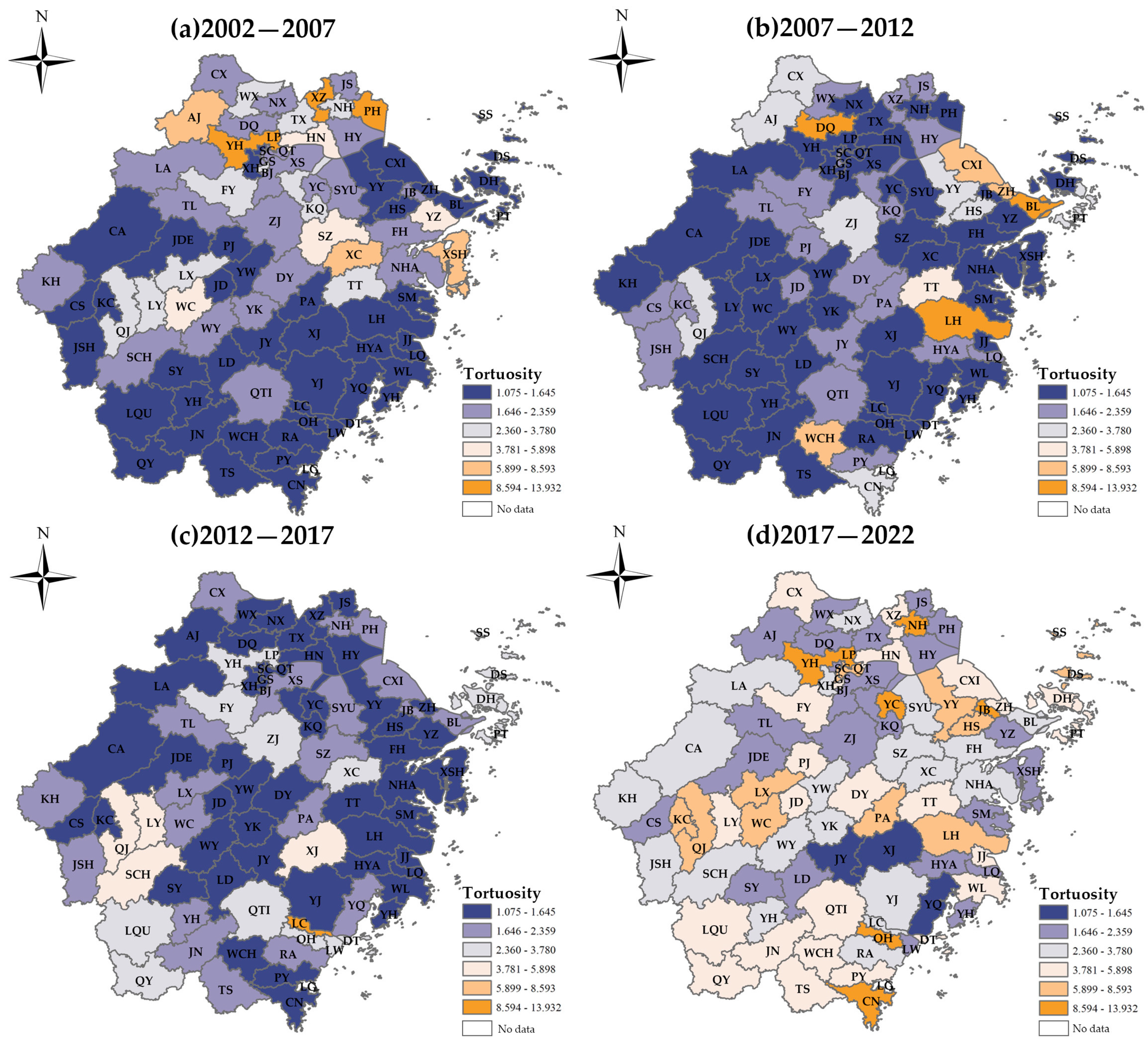
(1) LISA time path analysis results indicated that, overall, the county-level carbon emissions in Zhejiang Province from 2002 to 2022 exhibited strong local spatial structure stability, with an upward trend in this stability. Spatially, the most robust regional spatial structural stability of carbon emissions was found in western Wenzhou and Lishui in southern Zhejiang, Quzhou in Zhejiang’s west, and western Taizhou and western Hangzhou, showing a trend of spreading from south and west Zhejiang to northern and eastern Zhejiang. The spatial pattern of carbon emissions in the county areas of Zhejiang Province possesses specific spatial integrative characteristics. However, this integrative tendency is generally weakening, with non-synergistic growth predominantly exhibiting a fragmented pattern.
(2) The spatio-temporal transition results from the Moran’s scatterplot indicated that the most common transition was Type IV, with solid stability in the Moran’s scatterplot. This suggests a relatively high spatial accumulation of carbon emissions in the county areas of Zhejiang Province, a high degree of path dependence in carbon emissions spatial aggregation, and relative stability in the spatial structure of carbon emissions. This reflects that spillover effects from surrounding regions influence local county areas less, and internal factors significantly impact changes in their carbon emission spatial structure.
(3) A consistent “northeast–southwest” pattern emerged in the spatial distribution as the axis length varied. From 2002 to 2022, the centroid of county-level carbon emissions in Zhejiang Province varied within the range of 120.551° to 120.570° E and 29.555° to 29.591° N, moving generally northeastward and overall forming a ‘V’ shape. This indicated that the rate of increase in carbon emissions in the northeastern counties of Zhejiang was higher than the average, with the areas of high growth in overall carbon emissions still developing towards the northeast direction.
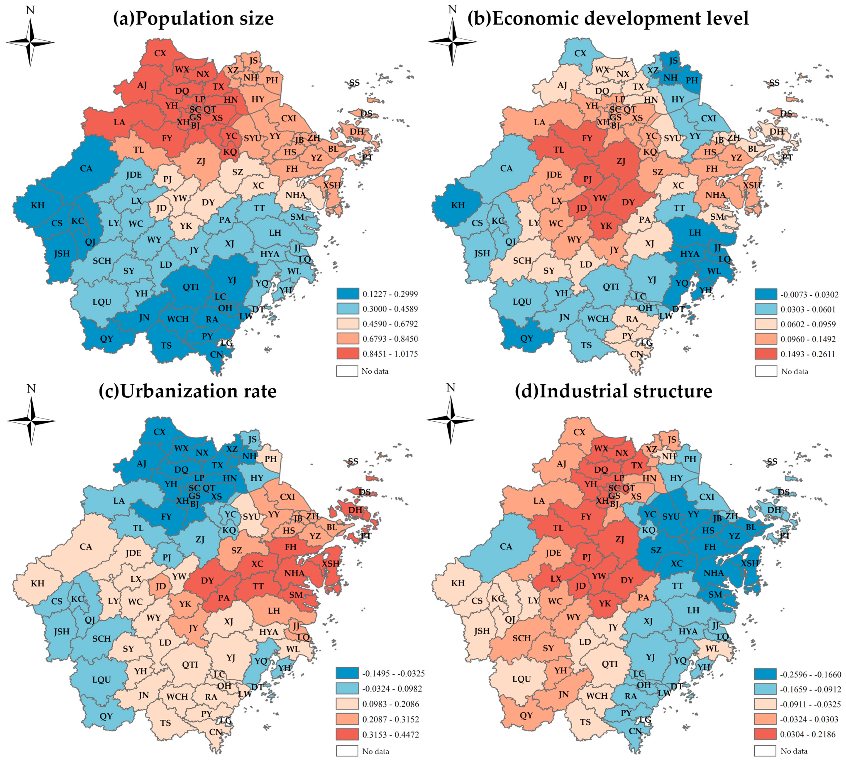
(4) The elements that influence carbon emissions vary significantly in terms of space and time. These factors, ranked in descending order of their degree of influence are population size, urbanization rate, industrial structure, and economic development level. Among these, population size, urbanization rate, and economic development level mainly promote carbon emissions, while industrial structure acts to suppress emissions. While Zhu [29] argued that the growth of the secondary industry has significantly worsened carbon emissions, our research shows that the secondary sector reduces carbon emissions. This finding aligns with the studies of Qi [17] and Yang [60].

5. Discussions

5.1. Implications

Exploring the spatio-temporal dynamics and determinants of carbon emissions in Zhejiang Province’s counties through the lens of spatio-temporal interactions helps in the detailed analysis of these emissions from a micro-perspective. This approach also offers a basis for developing tailored emission reduction policies. Drawing from empirical findings and relevant literature, we present the following insights:
(1) The results of the standard deviation ellipse indicated that the northeastern counties of Zhejiang have higher carbon emissions, while the LISA time path results showed that the spatial structure stability of carbon emissions in the southwestern counties of Zhejiang was the strongest, with counties such as Yinzhou and Xiaoshan having the lowest stability. Therefore, differentiated carbon governance measures need to be adopted for different regional countries. For the northeastern counties of Zhejiang, more attention should be paid to reducing the total carbon emissions, which can be achieved by enhancing technological innovation [60], promoting the development of low-carbon industries, and accelerating the modernization, integration, and transformation of traditional high-energy-consuming enterprises [17]. For the southwestern counties of Zhejiang such as Wencheng and Kaihua, more emphasis should be placed on the stability of carbon emissions through long-term, progressive (rather than short-term, volatile) policy guidance and control. At the same time, it is crucial to promote the transformation of the ecological economy in the long term, by optimizing the energy structure, such as increasing the proportion of clean energy and reducing reliance on fossil fuels, to ensure a stable decline in carbon emissions across counties [61].
(2) Spatio-temporal transitions indicated that the spatial agglomeration stability of carbon emissions in Zhejiang’s counties was strong, with weak influences between adjacent counties, and effective inter-regional linkages had not yet formed. Therefore, it is necessary to strengthen collaborative development between counties, breaking the highly stable spatial structure and path dependence of carbon emissions. Different counties have varying development modes and actual situations, which can complement each other’s advantages for joint development. This can be achieved by improving resource utilization efficiency, achieving regional coordinated development, and sharing ecological advantages [62]. Establishing a cross-regional cooperation mechanism can promote the sharing of experiences, technologies, and resources between different regions, strengthening collaborative efforts in carbon reduction. High-carbon emitting regions can collaborate with low-carbon emitting regions to reduce carbon emissions through resource transfer and technical support. Promoting cross-regional energy interaction and the development of the electricity network can enhance energy use efficiency and reduce carbon emissions [63].
(3) The factor of population size has a positive effect on carbon emissions, so attention should be paid to densely populated counties, transforming large population size and concentration into an advantage to improve per capita energy use efficiency. In addition, increased fiscal support, talent cultivation, and innovation and progress in low-carbon industries and products should be emphasized [64]. Similarly, the factor of economic development increases carbon emissions, so the quality of economic development should be emphasized over speed. Zhejiang should strategically implement the digital economy and promote industrial digital transformation. By optimizing production processes and improving energy use efficiency, energy consumption can be optimized, thus effectively controlling and reducing carbon emissions while promoting local economic development [65]. The urbanization rate factor exacerbates carbon dioxide emissions; hence, high-quality new urbanization development focusing on sustainable and eco-friendly urbanization growth models should be pursued, contrary to traditional demolition and construction urbanization patterns [66]. Meanwhile, the industrial structure factor inhibits carbon emissions, so the transformation of industrial structure should continue, vigorously developing the low-carbon and environmentally friendly tertiary industry, and accelerating the transformation of energy-intensive industries [31].

5.2. Limitations and Future Research Direction

This study comprehensively discusses the influencing factors of carbon emissions in the county areas of Zhejiang Province; however, due to the limited number of factors considered, more than this depth of research might be required. Future research will explore more relevant influencing factors on carbon emissions at the county level, aiming to provide differentiated strategies and suggestions for various counties. This study provides theoretical and empirical bases for formulating carbon emission reduction policies in Zhejiang Province. Nonetheless, the features of county regions vary considerably throughout Chinese provinces and cities. Consequently, other countries’ unique characteristics should inform the careful formulation of policies aimed at reducing carbon emissions. Future research directions should be more comprehensive than the study of carbon emissions in the county areas of Zhejiang Province. Still, they should extend to more provincial regions to explore county-level carbon emissions.

Author Contributions

Conceptualization, X.W. and Y.W.; Methodology, X.W. and Y.W.; Software, X.W.; Validation, X.W. and Y.W.; Formal analysis, H.Y.; Resources, H.Y.; Data curation, C.Z. and X.L.; Writing—original draft preparation, X.W.; Writing—review and editing, X.W. and Y.W.; Visualization, Y.L.; Supervision, Y.W.; Project administration, J.H.; Funding acquisition, X.W. and Y.W. All authors have read and agreed to the published version of the manuscript.

Funding

This research was supported by the Soft Science Research Plan Project of Zhejiang (No. 2024C35003), the Philosophy and Social Science Planning Project of Zhejiang (No. 24NDQN042YB), the Scientific Research and Nurturing Foundation of Hangzhou City University (No. J-202308), the Foundation of Hangzhou Federation of Humanities & Social Sciences (No. 2023HZSL-ZC011), the National Natural Science Foundation of China (No. 51878593), the Center for Balance Architecture, Zhejiang University (No. KH-20212946), the Artificial Intelligence Key Technologies R&D Program of Hangzhou (No. 2022AIZD0057), and the Strategic Research and Consulting Project of the Chinese Academy of Engineering (No. 2022-XZ-51).

Data Availability Statement

The data employed for this study were obtained from the Statistical Yearbook of Zhejiang and the China Emission Accounts and Dataset (CEADs). Access to these datasets is available at the following URLs: http://data.cnki.net and https://www.ceads.net (accessed on 6 August 2023).

Acknowledgments

The authors gratefully acknowledge the support of the funding.

Conflicts of Interest

All authors declare that the research was conducted in the absence of any commercial or financial relationships that could be construed as a potential conflict of interest.

Abbreviations

Attachment: To improve recognition in images, the names of counties are abbreviated. Below are the corresponding abbreviations for each county.
CountiesAbbreviations
ShangchengSC
GongshuGS
XihuXH
BinjiangBJ
XiaoshanXS
YuhangYHA
FuyangFY
LinanLA
TongluTL
ChunanCA
JiandeJDE
HaishuHS
JiangbeiJB
ZhenhaiZH
BeilunBL
YinzhouYZ
FenghuaFH
YuyaoYY
CixiCXI
XiangshanXSH
NinghaiNHA
LuchengLC
TaishunTS
RuianRA
YueqingYQ
NanhuNH
XiuzhouXZ
JiashanJS
HaiyanHY
HainingHN
PinghuPH
TongxiangTX
WuxingWX
NanxunNX
DeqingDQ
ChangxingCX
AnjiAJ
YuechengYC
KechengKQ
ShangyuSYU
ZhujiZJ
ShengzhouSZ
XinchangXC
WuchengWC
YongkangYK
KechengKC
QujiangQJ
JiangshanJSH
ChangshanCS
KaihuaKH
LongyouLY
DinghaiDH
PutuoPT
DaishanDS
ShengsiSS
JiaojiangJJ
HuangyanHYA
LuqiaoLQ
WenlingWL
LinhaiLH
YuhuanYHU
SanmenSM
TiantaiTT
XianjuXJ
LianduLD
LongquanLQU
LongwanLW
OuhaiOH
DongtouDT
YongjiaYJ
PingyangPY
CangnanCN
WenchengWCH
JindongJD
WuyiWY
PujiangPJ
PananPA
LanxiLX
YiwuYW
DongyangDY
QingtianQTI
YunheYH
QingyuanQY
JinyunJY
SuichangSCH
SongyangSY
JingningJN
LonggangLG

References

  1. Calvia, M. Worldwide Fluctuations in Carbon Emissions: Characterization and Synchronization. Clean. Prod. Lett. 2024, 6, 100054. [Google Scholar] [CrossRef]
  2. Oyewo, B.; Tauringana, V.; Tawiah, V.; Aju, O. Impact of Country Governance Mechanisms on Carbon Emissions Performance of Multinational Entities. J. Environ. Manag. 2024, 352, 120000. [Google Scholar] [CrossRef]
  3. Perdichizzi, S.; Buchetti, B.; Cicchiello, A.F.; Dal Maso, L. Carbon Emission and Firms’ Value: Evidence from Europe. Energy Econ. 2024, 131, 107324. [Google Scholar] [CrossRef]
  4. Perera, K.; Kuruppuarachchi, D.; Kumarasinghe, S.; Suleman, M.T. The Impact of Carbon Disclosure and Carbon Emissions Intensity on Firms’ Idiosyncratic Volatility. Energy Econ. 2023, 128, 107053. [Google Scholar] [CrossRef]
  5. Khan, A.A.; Mei, B.; Khan, S.U.; Ali, M.A.S.; Luo, J. Agri-Food Evolution and Carbon Emissions in Chinese Residential Consumption: A Life Cycle Analysis of Urban-Rural Disparities and Socioeconomic Influences. Environ. Impact Assess. Rev. 2024, 105, 107387. [Google Scholar] [CrossRef]
  6. Kotsompolis, G.; Konstantakis, K.N.; Xidonas, P.; Michaelides, P.G.; Thomakos, D.D. Climate Change Economics and the Determinants of Carbon Emissions’ Futures Returns: A Regime-Driven ARDL Model. Financ. Res. Lett. 2023, 58, 104485. [Google Scholar] [CrossRef]
  7. Zhou, K.; Yang, J.; Yang, T.; Ding, T. Spatial and Temporal Evolution Characteristics and Spillover Effects of China’s Regional Carbon Emissions. J. Environ. Manag. 2023, 325, 116423. [Google Scholar] [CrossRef] [PubMed]
  8. Liu, H.; Song, Y. Financial Development and Carbon Emissions in China since the Recent World Financial Crisis: Evidence from a Spatial-Temporal Analysis and a Spatial Durbin Model. Sci. Total Environ. 2020, 715, 136771. [Google Scholar] [CrossRef] [PubMed]
  9. Zhou, C.; Chen, X. Forecasting China’s Energy Consumption and Carbon Emission Based on Multiple Decomposition Strategy. Energy Strategy Rev. 2023, 49, 101160. [Google Scholar] [CrossRef]
  10. Dong, F.; Yu, B.; Hadachin, T.; Dai, Y.; Wang, Y.; Zhang, S.; Long, R. Drivers of Carbon Emission Intensity Change in China. Resour. Conserv. Recycl. 2018, 129, 187–201. [Google Scholar] [CrossRef]
  11. Pang, J.; Li, N.; Mu, H.; Zhang, M.; Zhao, H. Study on the Spatial Interaction between Carbon Emission Intensity and Shadow Economy in China. Sci. Total Environ. 2022, 813, 152616. [Google Scholar] [CrossRef] [PubMed]
  12. Zheng, J.; Mi, Z.; Coffman, D.; Milcheva, S.; Shan, Y.; Guan, D.; Wang, S. Regional Development and Carbon Emissions in China. Energy Econ. 2019, 81, 25–36. [Google Scholar] [CrossRef]
  13. He, Q.; Wei, F.; Deng, X.; Kong, F.; Li, C.; Yan, Z.; Qi, Y. Spatiotemporal Pattern of Carbon Productivity and Carbon Offset Potential in Chinese Counties. Sci. Total Environ. 2022, 846, 157153. [Google Scholar] [CrossRef]
  14. NBS. China Statistical Yearbook (County-Level); China Statistics Press: Beijing, China, 2018. [Google Scholar]
  15. Liu, X.; Jin, X.; Luo, X.; Zhou, Y. Quantifying the Spatiotemporal Dynamics and Impact Factors of China’s County-Level Carbon Emissions Using ESTDA and Spatial Econometric Models. J. Clean. Prod. 2023, 410, 137203. [Google Scholar] [CrossRef]
  16. Zhao, J.; Chen, Y.; Ji, G.; Wang, Z. Residential Carbon Dioxide Emissions at the Urban Scale for County-Level Cities in China: A Comparative Study of Nighttime Light Data. J. Clean. Prod. 2018, 180, 198–209. [Google Scholar] [CrossRef]
  17. Qi, H.; Shen, X.; Long, F.; Liu, M.; Gao, X. Spatial–Temporal Characteristics and Influencing Factors of County-Level Carbon Emissions in Zhejiang Province, China. Environ. Sci. Pollut. Res. 2022, 30, 10136–10148. [Google Scholar] [CrossRef] [PubMed]
  18. Duman, Z.; Mao, X.; Cai, B.; Zhang, Q.; Chen, Y.; Gao, Y.; Guo, Z. Exploring the Spatiotemporal Pattern Evolution of Carbon Emissions and Air Pollution in Chinese Cities. J. Environ. Manag. 2023, 345, 118870. [Google Scholar] [CrossRef]
  19. Liu, X.; Xu, H.; Zhang, M. The Effects of Urban Expansion on Carbon Emissions: Based on the Spatial Interaction and Transmission Mechanism. J. Clean. Prod. 2024, 434, 140019. [Google Scholar] [CrossRef]
  20. Zhang, Y.; Lin, W.; Ren, E.; Yu, Y. Evaluation of Spatial Distribution of Carbon Emissions from Land Use and Environmental Parameters: A Case Study in the Yangtze River Delta Demonstration Zone. Ecol. Indic. 2024, 158, 111496. [Google Scholar] [CrossRef]
  21. Soares, T.C.; Fernandes, E.A.; Toyoshima, S.H. The CO2 Emission Gini Index and the Environmental Efficiency: An Analysis for 60 Leading World Economies. EconomiA 2018, 19, 266–277. [Google Scholar] [CrossRef]
  22. Williams, R.G.; Ceppi, P.; Roussenov, V.; Katavouta, A.; Meijers, A.J.S. The Role of the Southern Ocean in the Global Climate Response to Carbon Emissions. Phil. Trans. R. Soc. A. 2023, 381, 20220062. [Google Scholar] [CrossRef] [PubMed]
  23. Qu, H.; You, C.; Feng, C.-C.; Guo, L. Spatial Responses of Ecosystem Services to Carbon Emission Efficiency Based on Spatial Panel Models in the Yangtze River Economic Belt. J. Clean. Prod. 2024, 434, 139953. [Google Scholar] [CrossRef]
  24. Quan, C.; Cheng, X.; Yu, S.; Ye, X. Analysis on the Influencing Factors of Carbon Emission in China’s Logistics Industry Based on LMDI Method. Sci. Total Environ. 2020, 734, 138473. [Google Scholar] [CrossRef] [PubMed]
  25. González, P.F.; Presno, M.J.; Landajo, M. Tracking the Change in Spanish Greenhouse Gas Emissions through an LMDI Decomposition Model: A Global and Sectoral Approach. J. Environ. Sci. 2024, 139, 114–122. [Google Scholar] [CrossRef] [PubMed]
  26. Khodakarami, L.; Pourmanafi, S.; Soffianian, A.R.; Lotfi, A. Modeling Spatial Distribution of Carbon Sequestration, CO2 Absorption, and O2 Production in an Urban Area: Integrating Ground-Based Data, Remote Sensing Technique, and GWR Model. Earth Space Sci. 2022, 9, e2022EA002261. [Google Scholar] [CrossRef]
  27. Li, W.; Dong, F.; Ji, Z. Research on Coordination Level and Influencing Factors Spatial Heterogeneity of China’s Urban CO2 Emissions. Sustain. Cities Soc. 2021, 75, 103323. [Google Scholar] [CrossRef]
  28. Nosheen, M.; Abbasi, M.A.; Iqbal, J. Analyzing Extended STIRPAT Model of Urbanization and CO2 Emissions in Asian Countries. Environ. Sci. Pollut. Res. 2020, 27, 45911–45924. [Google Scholar] [CrossRef]
  29. Zhu, E.; Qi, Q.; Chen, L.; Wu, X. The Spatial-Temporal Patterns and Multiple Driving Mechanisms of Carbon Emissions in the Process of Urbanization: A Case Study in Zhejiang, China. J. Clean. Prod. 2022, 358, 131954. [Google Scholar] [CrossRef]
  30. NBS. China Statistical Yearbook (County-Level); China Statistics Press: Beijing, China, 2022. [Google Scholar]
  31. Xia, C.; Li, Y.; Ye, Y.; Shi, Z.; Liu, J. Decomposed Driving Factors of Carbon Emissions and Scenario Analyses of Low-Carbon Transformation in 2020 and 2030 for Zhejiang Province. Energies 2017, 10, 1747. [Google Scholar] [CrossRef]
  32. Rey, S.J. Spatial Empirics for Economic Growth and Convergence. Geogr. Anal. 2001, 33, 195–214. [Google Scholar] [CrossRef]
  33. Gui, D.; He, H.; Liu, C.; Han, S. Spatio-Temporal Dynamic Evolution of Carbon Emissions from Land Use Change in Guangdong Province, China, 2000–2020. Ecol. Indic. 2023, 156, 111131. [Google Scholar] [CrossRef]
  34. Jiang, H.; Yin, J.; Qiu, Y.; Zhang, B.; Ding, Y.; Xia, R. Industrial Carbon Emission Efficiency of Cities in the Pearl River Basin: Spatiotemporal Dynamics and Driving Forces. Land 2022, 11, 1129. [Google Scholar] [CrossRef]
  35. Ye, X.; Rey, S. A Framework for Exploratory Space-Time Analysis of Economic Data. Ann. Reg. Sci. 2013, 50, 315–339. [Google Scholar] [CrossRef]
  36. Razzaq, A.; Sharif, A.; Yang, X.; Dogan, E. Influence Mechanism of Electricity Price Distortion on Industrial Green Transformation: A Spatial Analysis of Chinese Regions. Energy Econ. 2024, 130, 107308. [Google Scholar] [CrossRef]
  37. Güneyli, H.; Saleh Ahmed, S.M. Detecting Abnormal Seismic Activity Areas of Anatolian Plate and Deformation Directions Using Python Geospatial Libraries. Heliyon 2023, 9, e14394. [Google Scholar] [CrossRef] [PubMed]
  38. Lefever, D.W. Measuring Geographic Concentration by Means of the Standard Deviational Ellipse. Am. J. Sociol. 1926, 32, 88–94. [Google Scholar] [CrossRef]
  39. Talkhabi, H.; Ghalehteimouri, K.J.; Mehranjani, M.S.; Zanganeh, A.; Karami, T. Spatial and Temporal Population Change in the Tehran Metropolitan Region and Its Consequences on Urban Decline and Sprawl. Ecol. Inform. 2022, 70, 101731. [Google Scholar] [CrossRef]
  40. Qin, Q.; Yan, H.; Li, B.; Lv, W.; Wasif Zafar, M. A Novel Temporal-Spatial Decomposition on Drivers of China’s Carbon Emissions. Gondwana Res. 2022, 109, 274–284. [Google Scholar] [CrossRef]
  41. Tang, D.; Ma, T.; Li, Z.; Tang, J.; Bethel, B. Trend Prediction and Decomposed Driving Factors of Carbon Emissions in Jiangsu Province during 2015–2020. Sustainability 2016, 8, 1018. [Google Scholar] [CrossRef]
  42. Wang, S.; Ma, Y. Influencing Factors and Regional Discrepancies of the Efficiency of Carbon Dioxide Emissions in Jiangsu, China. Ecol. Indic. 2018, 90, 460–468. [Google Scholar] [CrossRef]
  43. Zhang, F.; Deng, X.; Phillips, F.; Fang, C.; Wang, C. Impacts of Industrial Structure and Technical Progress on Carbon Emission Intensity: Evidence from 281 Cities in China. Technol. Forecast. Soc. Chang. 2020, 154, 119949. [Google Scholar] [CrossRef]
  44. Huang, Y.; Matsumoto, K. Drivers of the Change in Carbon Dioxide Emissions under the Progress of Urbanization in 30 Provinces in China: A Decomposition Analysis. J. Clean. Prod. 2021, 322, 129000. [Google Scholar] [CrossRef]
  45. Zhang, H.; Zhang, X.; Yuan, J. Driving Forces of Carbon Emissions in China: A Provincial Analysis. Environ. Sci. Pollut. Res. 2021, 28, 21455–21470. [Google Scholar] [CrossRef] [PubMed]
  46. Liu, Y.; Jiang, Y.; Liu, H.; Li, B.; Yuan, J. Driving Factors of Carbon Emissions in China’s Municipalities: A LMDI Approach. Environ. Sci. Pollut. Res. 2022, 29, 21789–21802. [Google Scholar] [CrossRef]
  47. Shum, W.Y.; Ma, N.; Lin, X.; Han, T. The Major Driving Factors of Carbon Emissions in China and Their Relative Importance: An Application of the LASSO Model. Front. Energy Res. 2021, 9, 726127. [Google Scholar] [CrossRef]
  48. Sitorus, F.; Brito-Parada, P.R. A Multiple Criteria Decision Making Method to Weight the Sustainability Criteria of Renewable Energy Technologies under Uncertainty. Renew. Sustain. Energy Rev. 2020, 127, 109891. [Google Scholar] [CrossRef]
  49. Hohl, A.; Lotfata, A. Modeling Spatiotemporal Associations of Obesity Prevalence with Biking, Housing Cost and Green Spaces in Chicago, IL, USA, 2015–2017. J. Transp. Health 2022, 26, 101412. [Google Scholar] [CrossRef]
  50. Ariken, M.; Zhang, F.; Chan, N.W.; Kung, H. Coupling Coordination Analysis and Spatio-Temporal Heterogeneity between Urbanization and Eco-Environment along the Silk Road Economic Belt in China. Ecol. Indic. 2021, 121, 107014. [Google Scholar] [CrossRef]
  51. Mohammadnazar, A.; Mahdinia, I.; Ahmad, N.; Khattak, A.J.; Liu, J. Understanding How Relationships between Crash Frequency and Correlates Vary for Multilane Rural Highways: Estimating Geographically and Temporally Weighted Regression Models. Accid. Anal. Prev. 2021, 157, 106146. [Google Scholar] [CrossRef]
  52. Bui Minh, T.; Nguyen Ngoc, T.; Bui Van, H. Relationship between Carbon Emissions, Economic Growth, Renewable Energy Consumption, Foreign Direct Investment, and Urban Population in Vietnam. Heliyon 2023, 9, e17544. [Google Scholar] [CrossRef]
  53. Rehman, E.; Rehman, S. Modeling the Nexus between Carbon Emissions, Urbanization, Population Growth, Energy Consumption, and Economic Development in Asia: Evidence from Grey Relational Analysis. Energy Rep. 2022, 8, 5430–5442. [Google Scholar] [CrossRef]
  54. Gershon, O.; Asafo, J.K.; Nyarko-Asomani, A.; Koranteng, E.F. Investigating the Nexus of Energy Consumption, Economic Growth and Carbon Emissions in Selected African Countries. Energy Strategy Rev. 2024, 51, 101269. [Google Scholar] [CrossRef]
  55. Balta-Ozkan, N.; Watson, T.; Mocca, E. Spatially Uneven Development and Low Carbon Transitions: Insights from Urban and Regional Planning. Energy Policy 2015, 85, 500–510. [Google Scholar] [CrossRef]
  56. Wojewodzki, M.; Wei, Y.; Cheong, T.S.; Shi, X. Urbanisation, Agriculture and Convergence of Carbon Emissions Nexus: Global Distribution Dynamics Analysis. J. Clean. Prod. 2023, 385, 135697. [Google Scholar] [CrossRef]
  57. Raihan, A.; Ibrahim, S.; Muhtasim, D.A. Dynamic Impacts of Economic Growth, Energy Use, Tourism, and Agricultural Productivity on Carbon Dioxide Emissions in Egypt. World Dev. Sustain. 2023, 2, 100059. [Google Scholar] [CrossRef]
  58. Awan, A.; Alnour, M.; Jahanger, A.; Onwe, J.C. Do Technological Innovation and Urbanization Mitigate Carbon Dioxide Emissions from the Transport Sector? Technol. Soc. 2022, 71, 102128. [Google Scholar] [CrossRef]
  59. Mehmood, S.; Zaman, K.; Khan, S.; Ali, Z.; Khan, H.U.R. The Role of Green Industrial Transformation in Mitigating Carbon Emissions: Exploring the Channels of Technological Innovation and Environmental Regulation. Energy Built Environ. 2024, 5, 464–479. [Google Scholar] [CrossRef]
  60. Yang, L.; Xia, H.; Zhang, X.; Yuan, S. What Matters for Carbon Emissions in Regional Sectors? A China Study of Extended STIRPAT Model. J. Clean. Prod. 2018, 180, 595–602. [Google Scholar] [CrossRef]
  61. Tao, A. Research on the Realization Path of Carbon Emission Reduction in Zhejiang Province. Energy Rep. 2022, 8, 501–506. [Google Scholar] [CrossRef]
  62. Zeng, S.; Wang, M. Theoretical and Empirical Analyses on the Factors Affecting Carbon Emissions: Case of Zhejiang Province, China. Environ. Dev. Sustain. 2023, 25, 2522–2549. [Google Scholar] [CrossRef]
  63. Di, K.; Chen, W.; Zhang, X.; Shi, Q.; Cai, Q.; Li, D.; Liu, C.; Di, Z. Regional Unevenness and Synergy of Carbon Emission Reduction in China’s Green Low-Carbon Circular Economy. J. Clean. Prod. 2023, 420, 138436. [Google Scholar] [CrossRef]
  64. Ke, S.; Zhang, Z.; Wang, Y. China’s Forest Carbon Sinks and Mitigation Potential from Carbon Sequestration Trading Perspective. Ecol. Indic. 2023, 148, 110054. [Google Scholar] [CrossRef]
  65. Li, Z.; Lu, Z.; Xu, L.; Shi, Y.; Ma, Q.; Wu, Y.; Cao, Y.; Sheng, B. Examining the Decoupling of Economic Growth with Land Expansion and Carbon Emissions in Zhejiang Province, China. Land 2023, 12, 1618. [Google Scholar] [CrossRef]
  66. Chen, W.; Wang, G.; Xu, N.; Ji, M.; Zeng, J. Promoting or Inhibiting? New-Type Urbanization and Urban Carbon Emissions Efficiency in China. Cities 2023, 140, 104429. [Google Scholar] [CrossRef]
Figure 1. Schematic of research framework.
Land 13 00381 g001
Figure 2. Study area and administrative division.
Land 13 00381 g002
Figure 3. (ad) The relative lengths of LISA time paths in counties of Zhejiang Province from 2002 to 2022.
Land 13 00381 g003
Figure 4. (ad). The LISA time path curvature of counties in Zhejiang Province from 2002 to 2022.
Land 13 00381 g004
Figure 5. (ad). The LISA spatio-temporal transition direction of counties in Zhejiang Province from 2002 to 2022.
Land 13 00381 g005
Figure 6. The distribution of standard deviational ellipse and gravity center shift trajectory.
Land 13 00381 g006
Table 1. Definition of relevant indicators.
IndicatorsIndicator AbbreviationsConnotationUnit
Population sizePOPResident population by county at the end of the yearTen thousand
Economic development levelPGDPGDP per capitaTen thousand yuan
Urbanization rateURBRatio of urban population to resident population %
Industrial structureINSRatio of secondary sector output to GDP%
Table 2. Spatio-temporal transitions and spatial autocorrelation values for each period from 2002 to 2022.
Periodt/t + 1HHLHLLHLTypesNumberProportionsSt
2002–2007HH0.9750.0050.0050.015I70.0130.972
LH0.0200.9800.0000.000II70.013
LL0.0000.0050.9890.005III10.002
HL0.0630.0000.0630.875IV5200.972
2007–2012HH0.9730.0160.0000.011I40.0070.985
LH0.0000.9910.0090.000II40.007
LL0.0000.0001.0000.000III00.000
HL0.0250.0000.0250.950IV5260.985
2012–2017HH0.9770.0120.0000.012I40.0070.985
LH0.0180.9820.0000.000II40.007
LL0.0000.0001.0000.000III00.000
HL0.0450.0000.0000.955IV5260.985
2017–2022HH0.9710.0180.0060.006I70.0130.976
LH0.0170.9830.0000.000II40.007
LL0.0050.0050.9900.000III20.004
HL0.0470.0000.0470.907IV5210.976
Table 3. Spatio-temporal transition matrix and spatial cohesion value of each period.
YearCoordinates of Gravity CenterShift of Gravity CenterLong Axis/kmShort Axis/kmAngle°
LongitudesLatitudesOrientationsLength/km
2002120°55′15″ E29°55′52″ N 117.730165.9981.798
2007120°56′18″ E29°59′74″ Nnorthwestern5.542117.863161.4241.836
2012120°56′65″ E29°61′72″ Nnorthwestern0.746117.597160.7642.117
2017120°56′47″ E29°58′82″ Nsouthwestern0.285117.797161.8551.582
2022120°57′01″ E29°59′11″ Nnorthwestern0.853117.487161.9230.820
Table 4. Multicollinearity test.
VariablePopulation SizeLevel of Economic DevelopmentUrbanization RateIndustrial Structure
VIF1.1551.4111.2301.211
Table 5. Comparison of model evaluation metrics.
Model ParametersOLSGWRGTWR
R20.74870.85560.8846
Adjusted R20.73680.82030.8844
AICc−157.3643−180.3784−4784.4224
Disclaimer/Publisher’s Note: The statements, opinions and data contained in all publications are solely those of the individual author(s) and contributor(s) and not of MDPI and/or the editor(s). MDPI and/or the editor(s) disclaim responsibility for any injury to people or property resulting from any ideas, methods, instructions or products referred to in the content.

