Article

Multi-Temporal Passive and Active Remote Sensing for Agricultural Mapping and Acreage Estimation in Context of Small Farm Holds in Ethiopia

by
Tesfamariam Engida Mengesha
1,2,
Lulseged Tamene Desta
3,
Paolo Gamba
4,* and
Getachew Tesfaye Ayehu
3
1
Department of Remote Sensing and Application Research and Development, Ethiopian Space Science and Geospatial Institute (SSGI), Entoto Observatory and Research Center (EORC), Addis Ababa P.O. Box 33679, Ethiopia
2
Remote Sensing Department, Entoto Observatory and Research Center (EORC), Addis Ababa University, Addis Ababa P.O. Box 1176, Ethiopia
3
The Alliance of Bioversity International and CIAT, Addis Ababa P.O. Box 5689, Ethiopia
4
Telecommunications and Remote Sensing Laboratory, University of Pavia, 27100 Pavia, Italy
*
Author to whom correspondence should be addressed.
Land 2024, 13(3), 335; https://doi.org/10.3390/land13030335
Submission received: 30 January 2024 / Revised: 1 March 2024 / Accepted: 2 March 2024 / Published: 6 March 2024

Abstract

:
In most developing countries, smallholder farms are the ultimate source of income and produce a significant portion of overall crop production for the major crops. Accurate crop distribution mapping and acreage estimation play a major role in optimizing crop production and resource allocation. In this study, we aim to develop a spatio–temporal, multi-spectral, and multi-polarimetric LULC mapping approach to assess crop distribution mapping and acreage estimation for the Oromia Region in Ethiopia. The study was conducted by integrating data from the optical and radar sensors of sentinel products. Supervised machine learning algorithms such as Support Vector Machine, Random Forest, Classification and Regression Trees, and Gradient Boost were used to classify the study area into five first-class common land use types (built-up, agriculture, vegetation, bare land, and water). Training and validation data were collected from ground and high-resolution images and split in a 70:30 ratio. The accuracy of the classification was evaluated using different metrics such as overall accuracy, kappa coefficient, figure of metric, and F-score. The results indicate that the SVM classifier demonstrates higher accuracy compared to other algorithms, with an overall accuracy for Sentinel-2-only data and the integration of optical with microwave data of 90% and 94% and a kappa value of 0.85 and 0.91, respectively. Accordingly, the integration of Sentinel-1 and Sentinel-2 data resulted in higher overall accuracy compared to the use of Sentinel-2 data alone. The findings demonstrate the remarkable potential of multi-source remotely sensed data in agricultural acreage estimation in small farm holdings. These preliminary findings highlight the potential of using multi-source active and passive remote sensing data for agricultural area mapping and acreage estimation.

1. Introduction

The occurrence of climate variability, coupled with resource scarcity, social and political instability, pest outbreaks, and various other factors, has resulted in episodes of food insecurity in sub-Saharan Africa, placing the lives and livelihoods of the most disadvantaged communities at risk [1,2,3,4]. The agricultural system and landscape in sub-Saharan Africa are predominantly composed of smallholder farms that rely on rainfall to cultivate their crops [5,6,7]. Similarly, the agriculture system in Ethiopia is very complex, with 96% of the total cultivated area held by smallholders and producing a significant portion of the overall production for the major crops [8,9]. According to the Central Statistical Agency (CSA), agricultural farms in Ethiopia are divided into two main categories: smallholder farms, which are farms with an area of less than 25.2 hectares, and large commercial farms, which are farms with an area of more than 25.2 hectares. The majority of farming systems in Ethiopia are smallholder farms, with the majority focused on subsistence agriculture, producing primarily for their consumption. In general, only 40% of smallholders cultivate more than 0.90 hectares, and these small-sized farms make up the majority of the total cultivated area in the country [9,10,11].
The agricultural mapping and estimation of crop production area of smallholder farms provides quantitative information for forecasting food security in communities [12]. Crop maps are important inputs for crop inventory production and yield estimation, and they can help farmers implement effective farm management practices and improve their livelihood [13]. However, there are no cropland extent maps at national and local scales in Ethiopia, particularly in the study area, that are regularly updated. The availability of digital crop extent map services may fill a gap in the country’s current crop monitoring services by providing accurate, high-resolution, and regularly updated cropland area maps, as well as associated datasets [14].
The assessment of agricultural food production in Ethiopia, which relies on measuring crop area and crop yield, is particularly challenging due to the inadequacy and lack of accuracy in agricultural statistics, which is primarily attributable to inadequate organization and analysis of the data. Furthermore, agricultural statistics in Ethiopia are given at a coarse level, based on administrative units, affecting the accuracy and quality of the data [15,16]. Reliable information on where crops are grown, and their distribution patterns are essential for various purposes, including studying regional agriculture production, making informed political decisions, and enabling effective crop management. Accurately mapping agricultural crop distribution and estimating acreage play a significant role in optimizing crop production and resource allocation [17,18,19,20] and implementing and evaluating crop management strategies [21,22].
Remote sensing data are widely used for various applications in the agricultural domain, including soil property detection [23,24,25], crop type classification, and crop yield forecasting [26,27,28,29,30]. The information obtained from satellite images is dependent on the measurement of the electromagnetic energy reflected by different target features on the Earth’s surface [31]. However, it is crucial to consider atmospheric effects, as they can significantly influence the reflectance values received by the satellite sensor [31,32]. Several studies have highlighted the challenge of differentiating between land surface target features with varying spectral signatures [33,34,35]. It has been observed that even similar land surface target features can exhibit different spectral signatures, making accurate classification challenging. Furthermore, the issue of similar reflection characteristics among different land cover classes in a study area adds complexity to the classification process, especially when working solely with optical images. In the past, satellite data used to analyze and understand agricultural lands were too generalized and limited in their ability to capture the diverse characteristics of these landscapes [36,37,38]. However, with the development of medium-resolution European Space Agency Sentinel constellation’s products, there has been a significant improvement in the quality of spectral resolution as well as a substantial increase in spatial resolution. This enhancement in satellite capabilities has made it feasible to monitor smallholder farms in a more detailed and comprehensive manner [39,40,41,42].
While a single sensor’s data may not be sufficient to optimize target class separation, incorporating radar data into classification models improves mapping accuracies due to increased cloud cover, independent data availability, and the physical and structural properties of the microwave signal—information that complements spectra from multispectral sensors [43]. The integration of radar imagery alongside optical images has proven to be beneficial [44,45,46]. Specifically, the integration of data from Sentinel-2 and Sentinel-1 allows for a more comprehensive understanding of complex landscapes in agricultural areas [44,47,48]. By incorporating radar data, the problems associated with different spectral signatures for similar land surface target features can be significantly reduced. However, the integration of radar and optical imagery alone does not eliminate all issues. For example, the classification of water features can be problematic, as isolated water bodies might be mistakenly classified as bare land. Similarly, vacant lands can sometimes resemble agricultural or urban land cover classes, leading to misclassification. To overcome these specific challenges, researchers have explored the use of additional data sources, such as higher-resolution satellite imagery (e.g., a resolution of 5 m or finer). By exploiting these ancillary data sources, accurate training data can be obtained without the need for a field campaign, thus enhancing the separability between different land cover classes and improving classification accuracy.
Various studies have extensively discussed the challenges in remote sensing classification and have proposed various solutions: multi-source data fusion that includes the integration of radar and optical data, as well as the use of higher-resolution datasets and auxiliary sources for training data [43,49,50,51,52]. These approaches can solve problems related to varying spectral signatures and misclassification of land use land cover classes and improve the accuracy of the classification by employing advanced machine learning.
For agricultural mapping, numerous classifiers have been developed, with some of the most commonly employed being Support Vector Machines (SVM), Random Forest (RF), Gradient Tree Boosting (GTB), and Maximum Likelihood Classifiers [53,54,55,56,57,58,59,60]. Several studies have been conducted and tested to determine the most reasonable and accurate method among the machine learning classifiers used for LULC mapping [61,62,63]. Although the accuracy levels of each machine learning technique vary, it has been found that SVM and RF often provide more superior accuracy for classification than other classic classifier algorithms [64,65,66,67]. The major challenge in the application of these techniques for agricultural land mapping and acreage estimation is the lack of high spatial, temporal, and spectral information data. This is particularly important when considering smallholder farms [68].
Previous research has developed LULC maps with high spatial resolution at regional and local scales using commercial satellite data [69,70,71]. However, access to high-resolution, high-quality, and cloud-free satellite imagery is a challenge in many regions, particularly in the rainy season, which is the main agricultural season for Ethiopians. As a result, local planning agencies and governments lack adequate spatial information on smallholder farmers, which ultimately affects the monitoring of agricultural production and evaluation of the SDGs [12]. This is the reason for the selection of the study area in the Oromia regional state, which is known for its significant agricultural activity. The accurate delineation of agricultural land parcels and estimation of the areas provided by our approach will serve as important inputs for policymakers, agricultural planners, and land managers. The availability of such information supports targeted actions such as optimal resource allocation, land use planning, and crop yield prediction, thereby enhancing agricultural productivity and sustainability. The use of freely available multi-source imagery for agricultural mapping on small-scale farmlands is valuable for many developing countries with limited budgets for high-resolution data.
Therefore, by using the data from Sentinel-2 and Sentinel-1, this research aims to classify the study area into five common level-1 land use land covers and evaluate the potential of freely available sentinel products for mapping smallholder agricultural crop distribution and estimating acreage. In addition to investigating the suitability of sentinel products, the LULC classification techniques were tested to select the most accurate one for each investigated landscape [50,72,73]. The machine learning algorithms used in these experiments were RF, SVM, Classification and Regression Trees (CART), and GTB—chosen for their ability to discriminate between different classes, handle noisy data, and be applied with limited samples.

2. Materials and Methods

2.1. Study Area

The study was conducted in the Oromia region, Ethiopia, which is located geographically 7°32′45.736″ N and 40°38′4.866″ E. Oromia is one of Ethiopia’s 12 regional states, with the largest population and land area [74] (Figure 1). The region shares borders with several other regional states, including Amhara, Afar, Somali, Benishangul-Gumuz, Sidama, Southwest Region, and Central Region [75].
The Oromia region is characterized by a diverse and complex topography, which includes a variety of physiographic features that contribute to its unique landscape. These geographical features encompass mountains, rolling plateaus, river valleys, and plains area [76,77]. The study area climate is characterized by dry, tropical, and temperate climate zones with significantly varied amounts of annual precipitation between 410 and 2000 mm and temperatures between 18 and 39 °C [78].
It is the biggest crop-producing region, followed by Amhara and the South Nations and Nationality. The region’s main crop is cereals, which cover 84% of the crop area [79]. In productivity area coverage and abundance, teff, maize, wheat, and sorghum are the most grown cereal grains. Also, this area grows a lot of vegetables, red pepper, Ethiopian cabbage, green pepper, and root crops like potato, sweet potato, and onion.

2.2. Methodology

The objective of performing Land Use and Land Cover (LULC) classification is to identify and extract particular land cover features from remotely sensed images. Although all surface features are not pertinent to our analysis, we adopted five distinct classes such as agricultural/crop, built-up/settlement, vegetation cover, bare-land, and water bodies, to avoid the binary classification of all surface features [80,81]. The selection of these classes is based on their relevance in understanding the overall agricultural landscape and distribution within the region. The effectiveness of the classifiers was then assessed quantitatively at the comprehensive class level, encompassing the entire study area depicted in Figure 1. Figure 2 illustrates a flow chart diagram describing the methodology.
In this study, two sets of images are created, one containing optical imagery and one created from the selected optical and SAR bands. Then, the bands and indices from Sentinel-2 and Sentinel-1 were combined into a single image. This can be achieved by stacking the relevant bands and indices along the band dimension.
To classify agricultural areas in a small and fragmented farmland landscape within the study area, the integration of Sentinel-1 and Sentinel-2 data was performed on the Google Earth Engine (GEE) cloud computing platform [82]. To determine the input variables for the classifications, the most informative multispectral bands related to the targeted features are filtered. Additionally, the spectral indices calculated from the two images of optical and microwave bands are created. Initially, the classification of the study area was carried out based on S-2 images. After that, S-1 data were retrieved over the same study period. S-1 data are spatially and temporally filtered. Following that, a stack of S-1 images is formed, resulting in a multiband multidimensional composite image rich in relevant information for later classification operations. This composite image consists of 4 bands that include both vertical and horizontal polarization components, their respective ratios, and a modified normalized ratio. Sentinel-1 vertical and horizontal polarization datasets have been integrated with the Sentinel-2 bands and indices. Furthermore, the collected images were reduced to a single image by computing their median values, resulting in a composite image for classification. Then, the second classification was performed based on the two integrated datasets at the GEE platform [83,84].
Then, the accuracy of each machine learning was assessed using different accuracy assessment metrics. Following the classification and accuracy assessments, the study area’s agricultural land cover was quantified using an area estimation methodology. This involved determining the spatial extent of agricultural land within the study area by employing pixel-based analysis and an error-adjusted area estimation by using the map class as the stratum of the sample.

2.2.1. Data Acquisition and Pre-Processing

Satellite Dataset

In this study, Sentinel-2 and Sentinel-1 satellite products were utilized for agricultural area mapping and acreage estimation. Sentinel-2 provides high-resolution multispectral optical imagery [85]. It consists of twin satellites that provide global coverage with a five-day revisit frequency at the equator, with 13 bands ranging from visible to short-wave infrared (SWIR) and varying spatial resolutions of 10–60 m [86]. Data from Sentinel-2 are processed at several levels. Level-1C (L1C) reflectance images are provided at the Top Of the Atmosphere (TOA), and Level-2A (L2A) reflectance images are provided at the Bottom Of the Atmosphere (BOA), derived from the L1C parameters [87].
The Sentinel-1 mission consists of two polar-orbiting satellites, Sentinel-1A, and Sentinel-1B, with C-band synthetic aperture radar instruments that operate day and night and can acquire imagery under any weather or illumination conditions [88,89,90]. Each Sentinel-1 satellite has a 12-day repeat cycle and provides C-band images in both solitary and dual polarization. Sentinel-1 data are openly accessible for enabling a variety of Earth monitoring applications because they are all-weather capable and have a high spatial resolution (up to 10 m) [81,91]. In this study, we employed the Sentinel-2 BOA data and the Sentinel-1 ground range detected (GRD) interferometric wide swath (IW) product.

Reference and Ground Truth Dataset

To establish reliable reference and ground truth data for validation and training purposes, a combination of field survey measurements, high-resolution Planet Scope imagery, and Google Earth data was employed. Field survey measurements were conducted using Global Positioning System (GPS) instruments. These measurements involved collecting accurate location information at specific land cover within the study area, which was later used as ground truth data for accuracy assessment. High-resolution Planet Scope imagery, with a spatial resolution of 3 m, was acquired to obtain detailed information about the land cover types. This imagery was also used as a reference dataset for training the machine learning algorithms and validating the classification results. In addition to GPS data and Planate Scope, Google Earth data, containing updated satellite imagery and land cover information, was also utilized as a reference dataset for cross-validation. A total of 5764 ground GPS items and 1718 items from PlanetScope, together with Google Earth map points, were randomly collected for the main agricultural season (September 2020–February 2021) in the study area. This additional dataset helped to strengthen the confidence and accuracy of the classification results.

2.3. Image Processing

2.3.1. Band Selection

The first steps in image classification are the selection and resampling of the bands. This was necessary to ensure consistency and compatibility between different bands during the subsequent analyses. Based on the spectral characteristics of the study area and target features, appropriate bands from the Sentinel-2 imagery were selected for analysis. This study used 9 spectral bands, such as three visible bands and NIR, as well as four vegetation red-edge bands and two SWIR bands. To ensure spatial uniformity, red-edge (B5, B6, and B7) and SWIR (B11 and B12) were resampled from 20 m to 10 m spatial resolution by using nearest neighbor interpolation to align them with the 10 m spatial resolution bands [92,93,94,95]. The selection aimed to optimize the differentiation of the desired land cover classes.
Furthermore, the study area experiences heavy rain during the Meher season (cropping) season, in which cloud coverage poses a challenge for optical remote sensing data. As a result, it is crucial to apply cloud-masking techniques to mitigate the impact of cloud coverage in optical imagery [96,97]. However, cloud masking may result in information loss, particularly in agricultural areas where cloud cover can be persistent during the rainy season [98,99]. Therefore, by incorporating the Sentinel-1 radar images with the cloud-masked Sentinel-2 optical images, the radar data can compensate for the missing information caused by cloud coverage in the optical images [100,101,102].

2.3.2. Spectral Indices for LULC Detection

Various spectral indices were calculated from the selected optical bands to identify specific land cover characteristics and improve classification accuracy. In this study, the 10 commonly used indices include Normalized Difference Vegetation Index (NDVI) Equation (1), Enhanced Vegetation Index (EVI) Equation (2), Green Normalized Difference Vegetation Index (GNDVI) Equation (3), Bare Soil Index (BSI) Equation (4), tasseled cap wetness index (TCW) Equation (8), Tasseled cap greenness index (TCG) Equation (7), Modified Normalized Difference Water Index (MNDWI) Equation (6), and Normalized Difference Water Index (NDWI) Equation (5), were derived from the selected bands to enhance the LULC classification. In addition to indices from Sentinel-2, the most commonly used radar-derived index, such as the radar ratio index (VV/VH) Equation (9) and modified radar vegetation index (mRVI) Equation (10) [103,104], was developed from Sentinel-1 (Table 1).

2.4. Classification

Machine learning algorithms have proven to be effective in remote sensing applications, including land cover classification and mapping. Machine learning algorithms can learn patterns and relationships in the satellite data based on various features, such as spectral signatures, indices, and contextual information, allowing for the classification of different land cover types in the study area [117,118,119]. To perform LULC classification, the reflectance and polarization data with two images (Sentinel-2 and 1) bands were acquired for the Meher crop season between September 2020 and February 2021. In this research, we employed a random and stratified sampling technique to collect ground truth data for classification and adjusted agricultural land area estimation. To ensure an effective assessment of the classifier performance, the reference data were subdivided into two sets: 70% for training the classifiers and the remaining 30% for testing.
Four commonly used machine learning algorithms—RF, SVM, CART, and GTB [19,66,120,121,122,123]—were employed for the classification of the study area. The classification processes were carried out using both Sentinel-2 data alone and the integration of Sentinel-2 and Sentinel-1 data. To perform LULC classification, image pre-processing was performed to obtain reflectance and polarization data with two image bands that were acquired for the Meher crop season between September 2020 and February 2021. The training dataset, consisting of labeled pixels from high-resolution reference images and ground truth data, along with the selected spectral bands and indices, was used to train the machine learning models. The classifiers were trained to differentiate the five defined land cover classes based on their spectral signatures. The trained models were then applied to the entire study area to classify the unknown pixels into the respective land cover classes. This process involved assigning a predicted class label to each pixel based on its spectral characteristics and proximity to the labeled training pixels. In this study, the following classifiers were used for LULC classification:
Random Forest: RF is a widely used algorithm for land cover classification using remote sensing data due to its ability to handle outliers, perform well with high-dimensional datasets, achieve higher accuracy than other classifiers, and increase processing speed by selecting important variables. It is a decision tree-based ensemble learning method that combines a big ensemble regression and classification tree method [124]. The classification and prediction performance of the random forest classification model depends on the optimization of the two primary parameters called the number of trees (Ntree) and the number of features (Mtree) [125,126,127], which makes it more popular than other machine learning algorithms [128,129,130]. Recently, several studies have demonstrated that the use of RF in the field of remote sensing applications can achieve good results for the classification of LULC [131,132,133,134]. It can handle a wide range of data, including satellite imagery and numerical data [64,135].
Gradient Boosting: The concept of gradient boosting was introduced by Friedman [136]. GTB base model is a robust tree-based data mining model that is flexible for processing different types of data, such as continuous and discrete data [117,137]. It involves fitting a parameterized function to pseudo residuals using additive models in a sequential manner. In the case of Gradient Tree Boosting (GTB), a decision tree is employed as the base learner [138]. It maximizes high-order feature information, generalizes without scaling, and representations by iteratively combining weak learner ensembles into stronger ensembles. GTB outperforms other ensemble classifiers in classification accuracy by using negative gradient loss values in each iteration to fit regression tree residuals [139]. GTB has gained attention in LULC mapping due to its ability to handle imbalanced datasets. Its robustness to outliers makes it suitable for LULC mapping in complex landscapes with high overall accuracy [82,135,140].
Support Vector Machine: Support Vector Machines (SVM) is a non-parametric supervised classification algorithm designed to determine an optimal hyperplane for classifying various classes in the feature space [141,142]. It is based on the principle of risk minimization, which maximizes and separates the hyper-plane and data points closest to the hyperplane spectral angle mapper. The algorithm learns to differentiate between various classes by selecting the hyperplane that maximizes the difference between them [143,144]. In the context of LULC, SVM uses labeled training data, with each sample assigned to a distinct land use or land cover category [145].
Although the polynomial and radial basis function (RBF) kernels have been used commonly in remote sensing, RBF is the most commonly employed approach for LULC classification and gives a higher level of precision than the other classic methods. It requires a good kernel function to reliably build hyper-planes and reduce classification errors [146,147,148].
Classification and Regression Trees: The Classification and Regression Trees (CART) is a multipurpose machine learning algorithm that uses decision tree principles to address both regression and classification problems [149]. It is an accurate image classification technique that provides the advantages of simplicity and fast execution. However, the algorithm experiences overfitting in the decision tree and generates complicated trees [139]. It works by recursively partitioning the training data into smaller subsets using binary splits [150,151]. It recursively partitions the outcome, in this case, the spatial pattern of interest, into progressively homogeneous subgroups, similar to RF, based on information provided by the predictor variables [152,153]. Data partitioning proceeds in a stage-wise fashion, which means that earlier split values are not taken into account in successive partitions [154].

2.5. Accuracy Assessments

The accuracy of the classification results was evaluated by using two primary metrics, including (OA, Equation (11)), and kappa coefficient (Ka, Equation (12)). The OA represents the overall agreement between the predicted and reference datasets, while the kappa coefficient accounts for the agreement beyond what would be expected by chance alone [155]. In addition to the above, the error of omission and commission was calculated [156]. To provide a comprehensive assessment of the classification results and evaluate the class-wise accuracy, other evaluation metrics, such as F-score (Equation (13)) [157] and Figure of Merit (Fm, Equation (14)) [21], user and producer accuracy [158] were calculated. These metrics evaluate the overall quality of the classification, considering both omission and commission errors. Specifically:
O A = k = 1 n C k k n
where Ckk is the row and column k value of the confusion matrix cell and n represents the total number of classes on the map.
K a = N i = 1 j = i n d i j i = 1 j = 1 n r i c j N 2 i = 1 j = 1 n r i c j
where N is the number of pixels, r i and c j are the total number of rows and columns in the error matrix, n is the number of classes, and d i j is the diagonal elements of the confusion matrix
F - s c o r e = 2 P A U A P A + U A
where PA and UA are the producer and user accuracies, respectively;
F m = O A C e + O e + O A
where, C e   a n d   O e are commission and omission errors, respectively, and O A is the overall accuracy.

3. Results

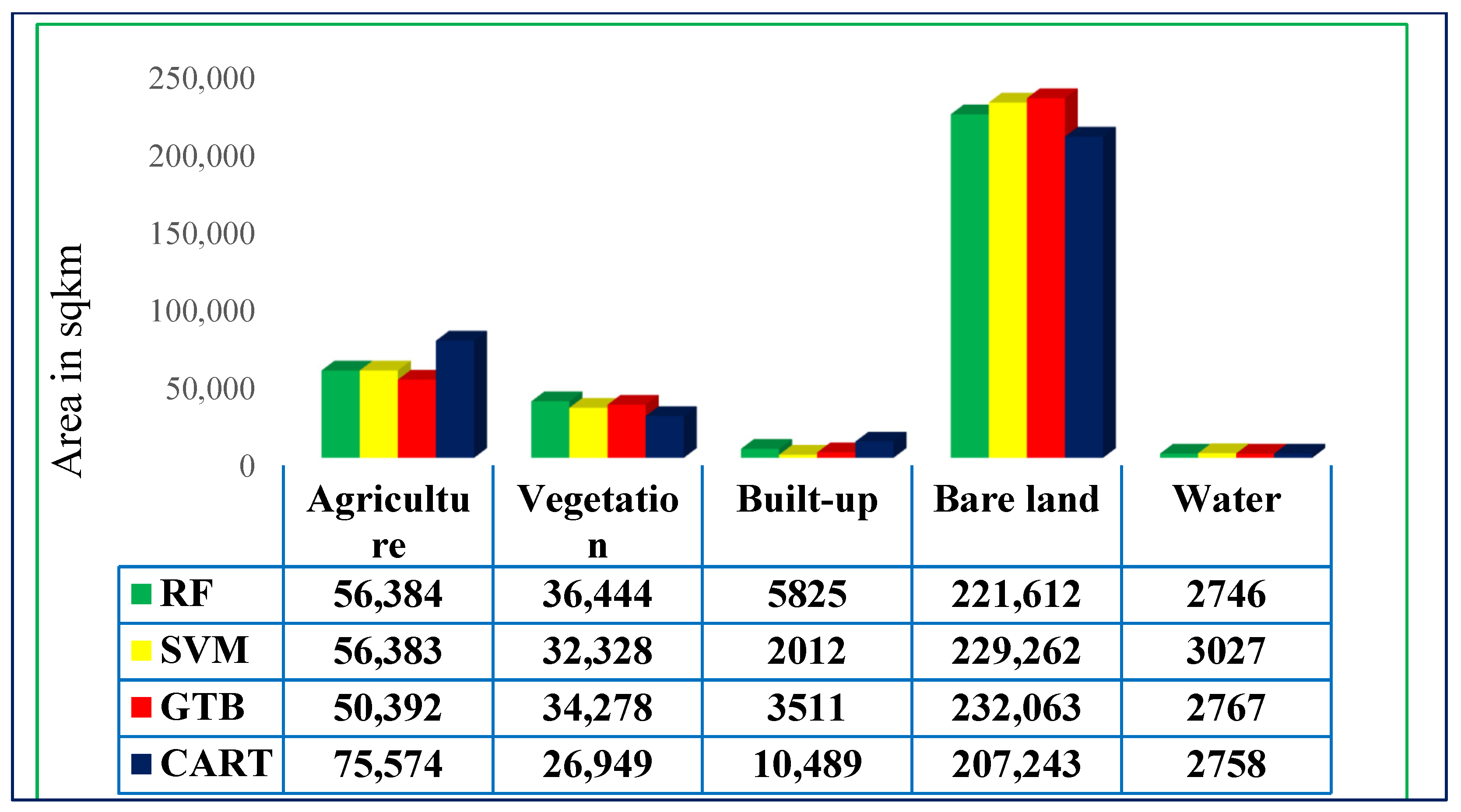
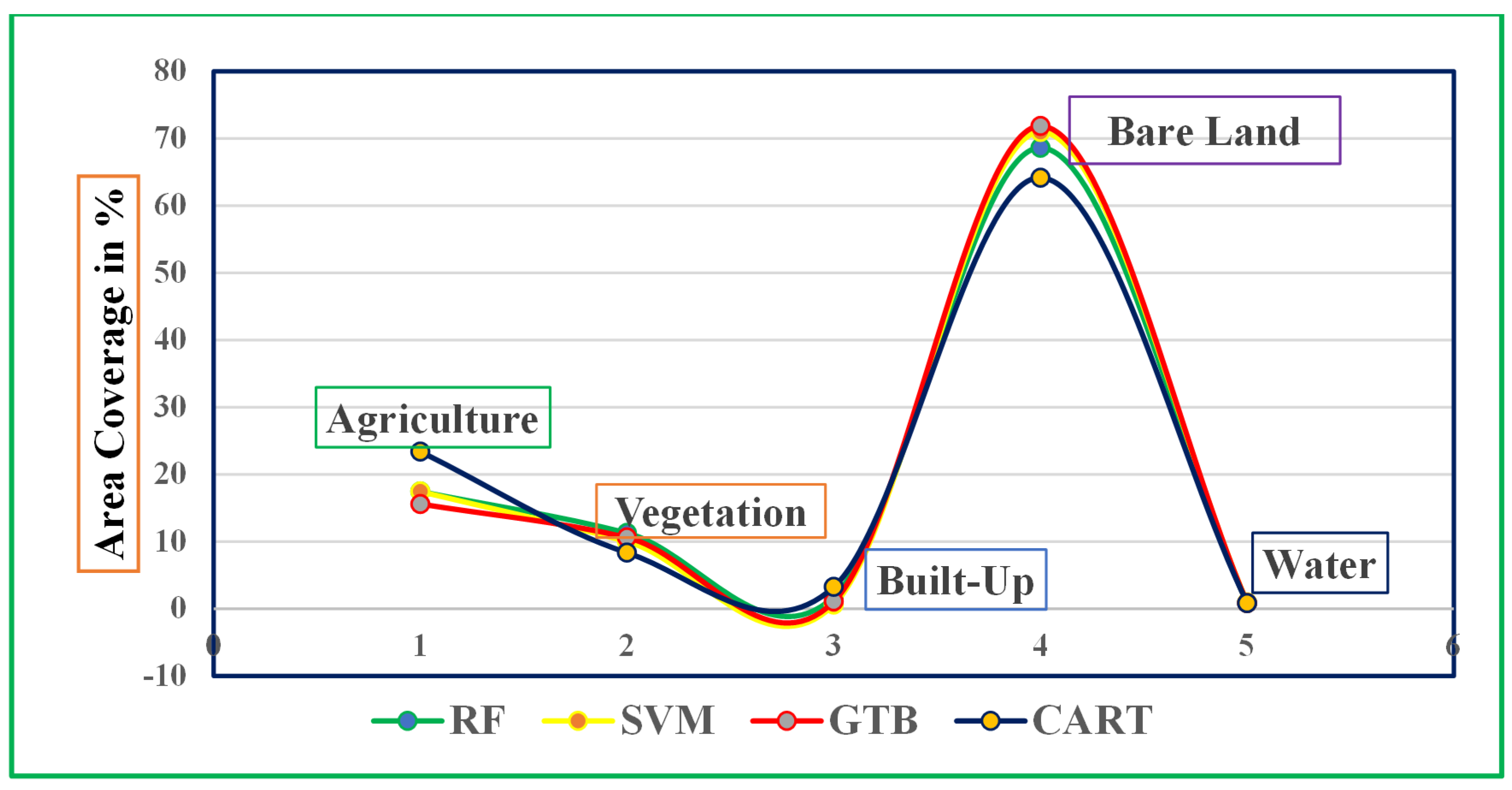
3.1. Land Use Land Cover Maps

This study examines the potential of freely available Sentinel-1 and Sentinel-2 datasets and, in the case of the Oromia region, evaluates the performance of machine learning algorithms on agricultural mapping and acreage estimation in small and fragmented farmlands. The result describes the classification results using MLAs of RF, SVM, GTB, and CART classifiers performed on Sentinel-2 (optical data) and the integration of Sentinel-2 with Sentinel-1 (microwave) data. The study combined ground truth from GPS field surveys and references from high-resolution PlanetScope and Google Earth images for accuracy assessments of the classifier. A total of 7482 ground sample points were collected, with the following distribution across classes: water (445), agriculture (1873), vegetation (564), bare land (2636), and built-up (1964). The variance in sample sizes is attributed to easy accessibility and the spatial distribution characteristics inherent to each land cover type. In this study, five classes of surface type were identified: Agriculture, Vegetation, Built-up, Bare land, and Water [159,160]. These classes were selected on the basis of the specific physical characteristics of the study area.
The initial land use and land cover (LULC) class was determined by analyzing class responses in the optical image bands. To improve classification accuracies, different spectral indices have been developed from the original bands of sentinel products. These indices, as stated in Table 1, give supplemental levels of information that are utilized as input for the classification algorithms. Previous research has proved the significance of these indexes for enhancing the accuracy of land use and land cover (LULC) analyses [82,161].
The second rule set is built upon this by incorporating the SAR VV and HV polarizations, along with related indices. After performing separate classifications using the optical approach and the synergistic approach, two thematic maps representing land use and land cover (LULC) were generated. These maps are displayed below, along with the results of the accuracy assessment.
Figure 3 presents the optical image classified maps obtained by the four machine learning algorithms (MLAs) for the Meher crop season in the study area. These LULC maps produced by Sentinel-2 data with RF, SVM, GTB, and CART models are presented in Figure 3a–d, respectively. The analysis of the graphical distribution of the classes in these maps reveals a consistent pattern in the major LULC units, with minor variations observed in the southern and some eastern areas, where the density of bare land is higher. This can be attributed to the region’s mountainous terrain and shrubland, which have been inaccessible to the public since the previous regime, as well as the dry climate leading to drought-affected areas in the region. From the map, it is observed that the CART algorithm-based map depicts more urban areas than other MLAs, which are represented by red color.
Additionally, minor dissimilarities are observed in the central area, where the largest land cover, agriculture, is located. Three classification algorithms, RF, SVM, and GTB, exhibit a consistent pattern in vegetation land cover with insignificant differences. Regarding the water cover, a relatively similar spatial extent is evident in the classification maps generated by all classifiers. The map below shows that the agricultural land cover class spatial pattern and extent were very similar for RF and GTB, Figure 3a,c.
The spatiotemporal availability of earth observation (EO) data, typically associated with vegetation greenness and crop growth in the visible and infrared portion of the electromagnetic spectrum, may be problematic when clouds prevent measuring the land surface [162,163]. The combination of optical and SAR data allows for a more comprehensive representation of biophysical and structural information on target objects, which in turn improves crop mapping [164,165].
In this study, we assess the performance of SAR and Optical integrated images for agricultural mapping and acreage estimation in small, fragmented farmlands. Therefore, LULC classification maps for S2 and S1 integration were generated using the same four supervised classification techniques. The findings of the study reveal a significant enhancement in the geographical distribution and visual interpretation of classification when utilizing combined imagery, as compared to relying solely on optical-only imagery.
The results show that, among the four algorithms examined, SVM, RF, and GTB demonstrated similar patterns in the homogeneity of class distribution related to Agriculture, vegetation cover, built-up area, water, and bare land. In contrast, the CART displayed marked discrepancies in the generated maps, primarily characterized by an overestimation of the built-up and agricultural classes, suggesting a lower level of precision in its results (Figure 4d).
The visual inspection of LULC revealed that the combined datasets could provide the best classification and were comparable more closely to current land covers based on SVM, RF, and GTB classification algorithms (Figure 4a–c). Most of the areas near the main southern parts and toward the eastern portion of the study area are highly covered with bare lands, also classified in the bare lands category in the classified results. Furthermore, the central and northwestern parts of the region are highly covered by agriculture and forest, respectively, and are also classified as agricultural and vegetation land cover. The map shows the types of LULC categories that exist in the area, with cultivated (Meher season) areas dominating the landscape next to the bare land. In contrast, water and settlements constitute a smaller percentage. The maps depict the many LULC classifications that exist in the area.

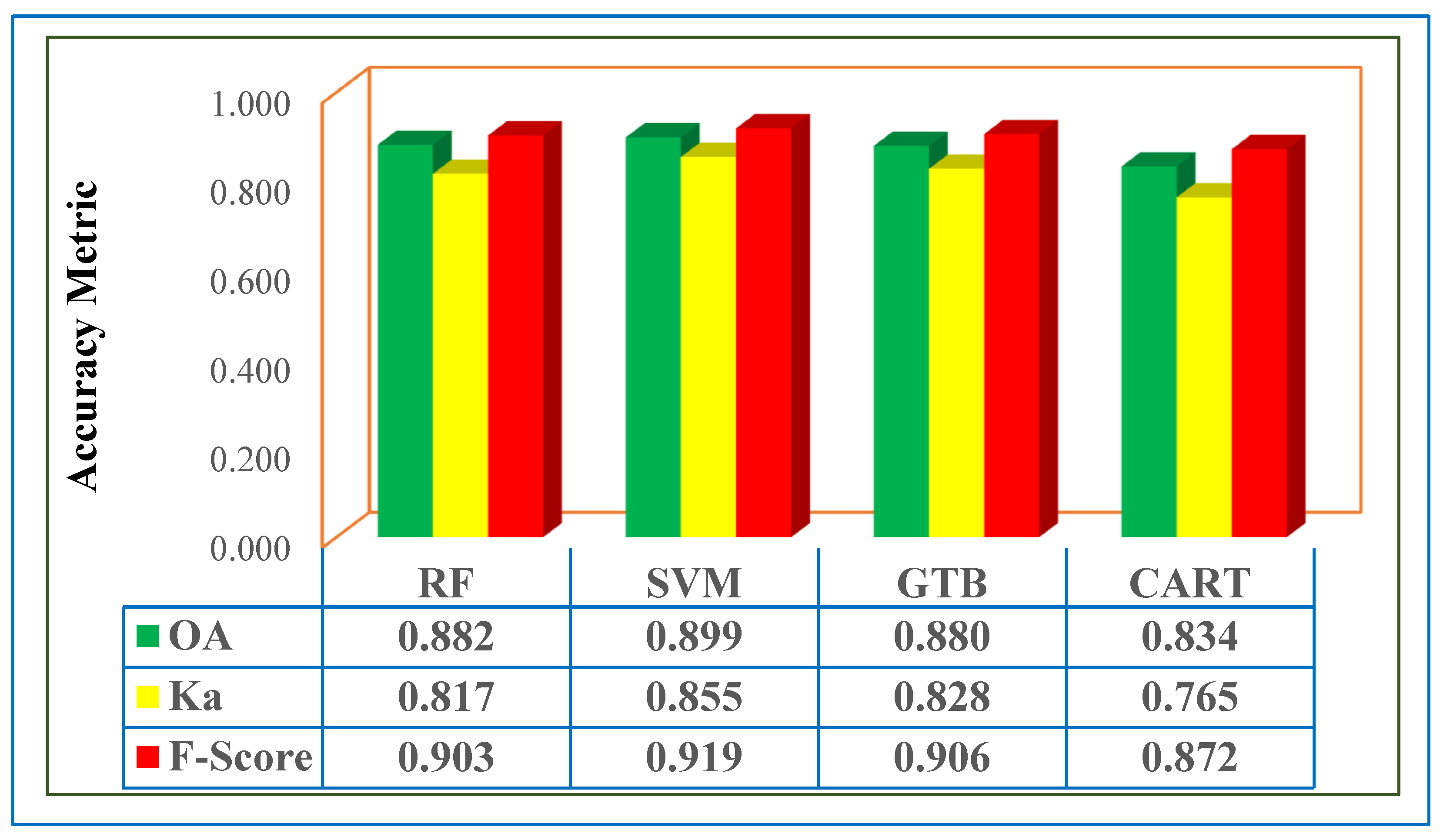
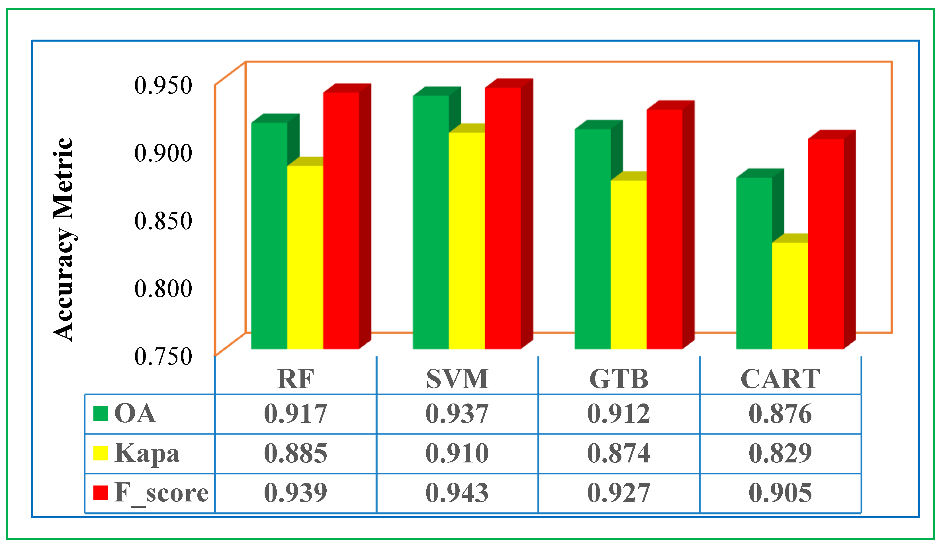
3.2. Quantitative Evaluation

The accuracy assessment of the classification was conducted in two approaches, directly by using the pixel classification and by using the class as strata to calculate unbiased class-wise accuracies, using various metrics such as overall accuracy, kappa coefficient, f-score, and figure of merit. In order to enhance classification accuracies, additional spectral indices are derived from the original bands of sentinel products [82,161]. The OA and Ka values, as well as the F-score and Fm measures, were computed from the confusion matrixes for RF, SVM, GTB, and CART in Table 2 and Table 3, respectively.
Despite the complex nature of the landscape and fragmented small plot sizes within the study area, which were classified into five distinct land use land cover (LULC) categories, the LULC maps produced by the MLAs showed high-accuracy assessment results. Figure 5 illustrates the comparative analysis of OA, Kapa, and F-Score achieved by all MLAs for LULC classification during the Meher season. For the Sentinel-2-only data, the selected algorithms exhibited notable performances, with the Support Vector Machine (SVM) classifier achieving the highest OA value of 89.9%, while the Classification and Regression Tree (CART) classifier attained the lowest OA value (83.4%) (Figure 5).
In the case of the RF and GTB classifier, employing optical-only imagery results in an average accuracy of 88%, while the CART classifier achieves an average accuracy of 83%.
In addition to overall accuracy, the accuracy assessment was carried out, which exhibits users (UA) and producer’s accuracy (PA) of each class of study area generated through SVM, RF, GTB, and CART (Table 2). The agricultural class of the LULC map generated by the SVM yields the highest UA values of 88%, while the CART yields less UA and values of 75%. The findings of the assessments also indicate the UA and PA of agricultural land use retrieved by RF and GTB are equal, measuring 83% and 80%, respectively. According to the results, SVM has the highest UA as compared to another classifier but less PA than RF and GTB. From Table 2, the accuracy metrics f-score for agricultural land cover is greater than 0.8 for RF, SVM, and GT, while it gave a lower result with the CART methods, which is 0.77. This indicates the potential of SVM, RF, and GTB for identifying and mapping agricultural areas within small and fragmented farmlands. The figure of merit for vegetation was over 95% for all classification algorithms.
There is variation in the accuracy of MLAs; this was confirmed by the previous study that demonstrates the highest achieved accuracies for each classifier, which vary depending on the type of imagery, input dataset, and training data configuration [135,166,167]. Furthermore, according to previous studies, any accuracies exceeding 85% are thresholds considered satisfactory for land use and land cover (LULC) applications [168,169,170]. Therefore, the findings of our analyses revealed that the obtained result is satisfactory for mapping and monitoring agricultural land in small and fragmented land farming systems in developing countries.
Additionally, the objective of this study was to determine the impact of S1-VH and S1-VV satellite images on enhancing the accuracy of classification in an area having small and fragmented farmlands. In the same ways, classification models, RF, SVM, GTB, and CART, were implemented on the integrated S1-VH and S1-VV polarization data along with the S2 satellite.
As compared to optical images alone, when SAR and optical imagery are combined, the accuracy of SVM increases to an average of 94%, while RF and GTB improve to an average of 92% and 91%, respectively (Figure 6). Similarly, the Classification and Regression Trees (CART) classifier also demonstrates the highest accuracy of 87% when utilizing the combined imagery.
Therefore, the synergistic imagery achieved the highest level of accuracy, indicating the incorporation of indices derived from Sentinel-1 images further improved the model performance marginally. Furthermore, the feature importance analysis highlighted the substantial contribution of radar data to the classification process. Previous studies prove that the addition of arithmetic operations of vertical and horizontal polarization as input for classification yields an increase in the accuracy of LULC classification approaches [81,171,172].
Furthermore, the classification accuracies at a class-wise level were evaluated using the validation dataset. Table 3 illustrates the class-wise accuracies (UA and PA) achieved by the SVM, RF, GTB, and CART models. These accuracies offer important perspectives into the specific contributions of each model in the detection and classification of various land cover in the study area, as indicated by the producer’s and user’s accuracies.
When compared with other classes, vegetation, built-up, and water bodies performed well, with more than 90% user and producer accuracy for the SVM, RF, and GTB models, while the CART gave UA and PA of less than 90% for the built-up class. Among the four classifiers tested, SVM and RF demonstrated the highest UA and PA values across all classes. While in both methodologies, SVM outperformed the other classifiers in terms of producer and user accuracy. SVM achieved a PA and UA exceeding 90% for all classes, while RF achieved a PA and UA exceeding 90% for all classes except for the bare land class, which had a UA of 88%. On the other hand, the GTB and CART classifiers showed higher accuracy (greater than 90%) for the vegetation and built-up area classes but had lower UA and PA for the other classes compared to SVM and RF. These results suggest that SVM and RF outperformed the other classifiers and are more suitable for agricultural mapping and estimating acreage in small and fragmented farmlands. The findings of the study confirmed similar studies that observe satisfactory levels of classification accuracy through the synergistic utilization of S2 multi-spectral and S1 polarization data [81,172].
Moreover, when comparing the accuracy between standalone Sentinel-2 classification and integrated Sentinel-2/Sentinel-1 classification, the results revealed that the integrated classification approach yielded higher accuracy. This improvement could be attributed to the complementary information provided by combining the optical and radar data sources, resulting in more robust and accurate classification results [47,173,174].

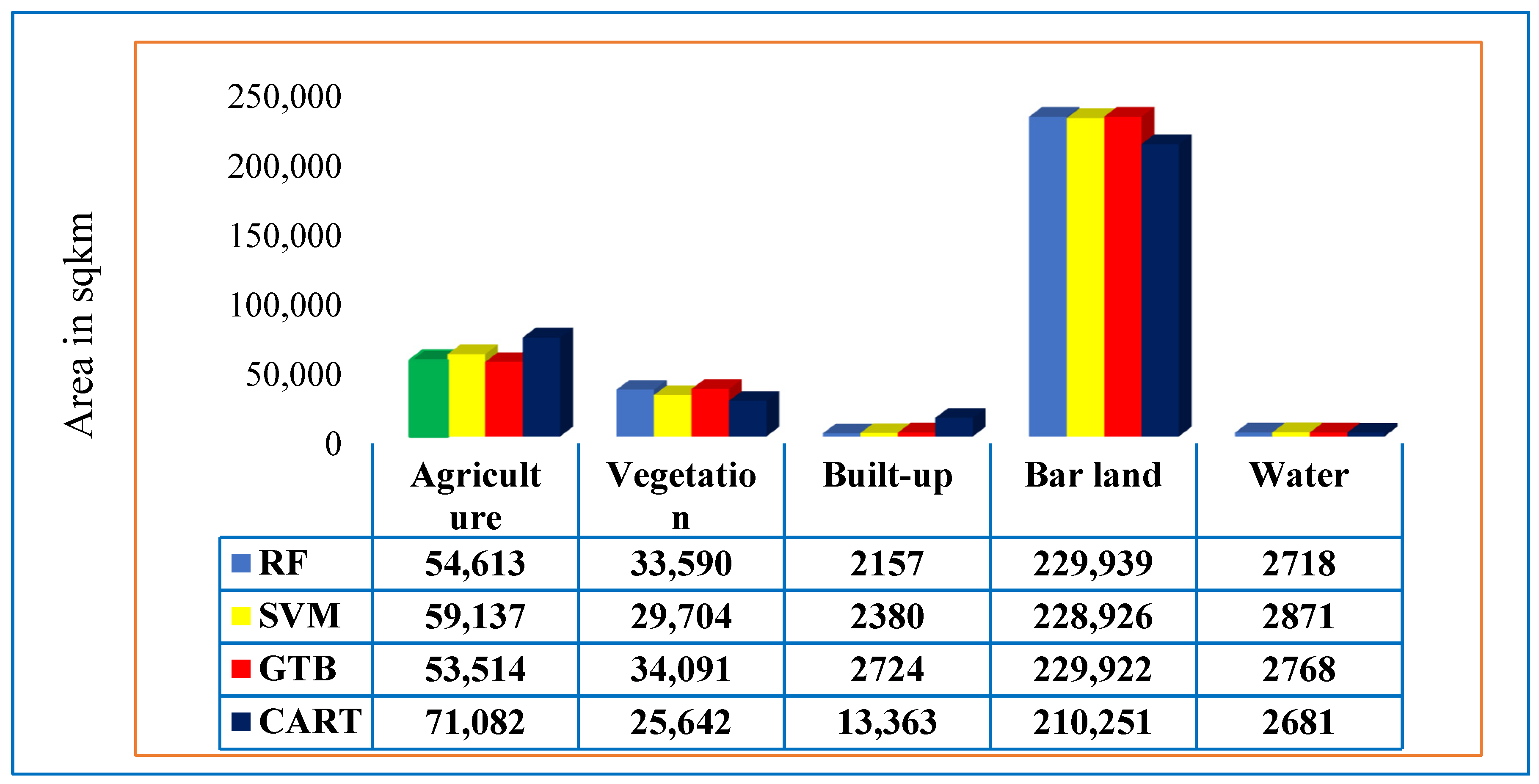
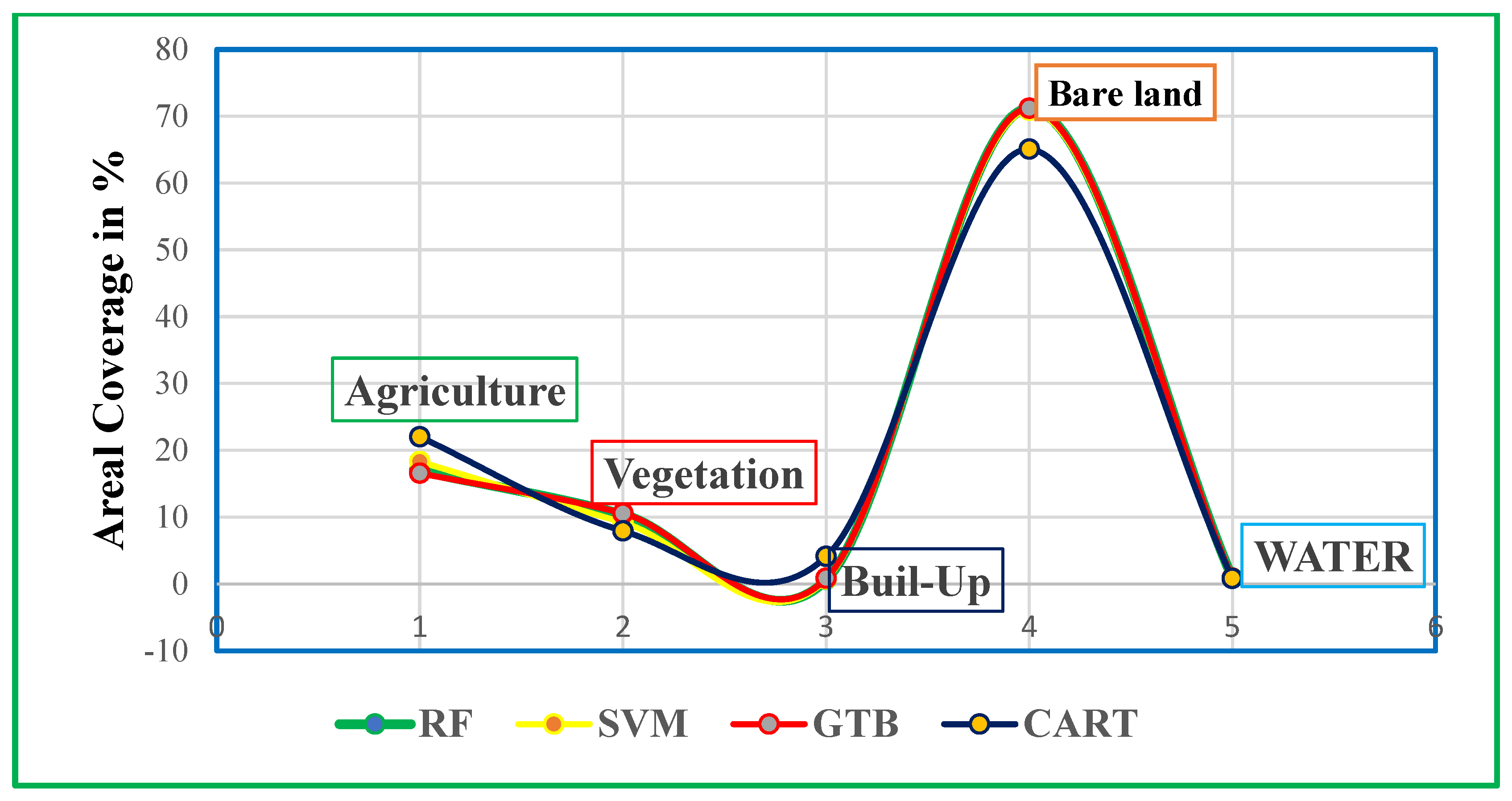
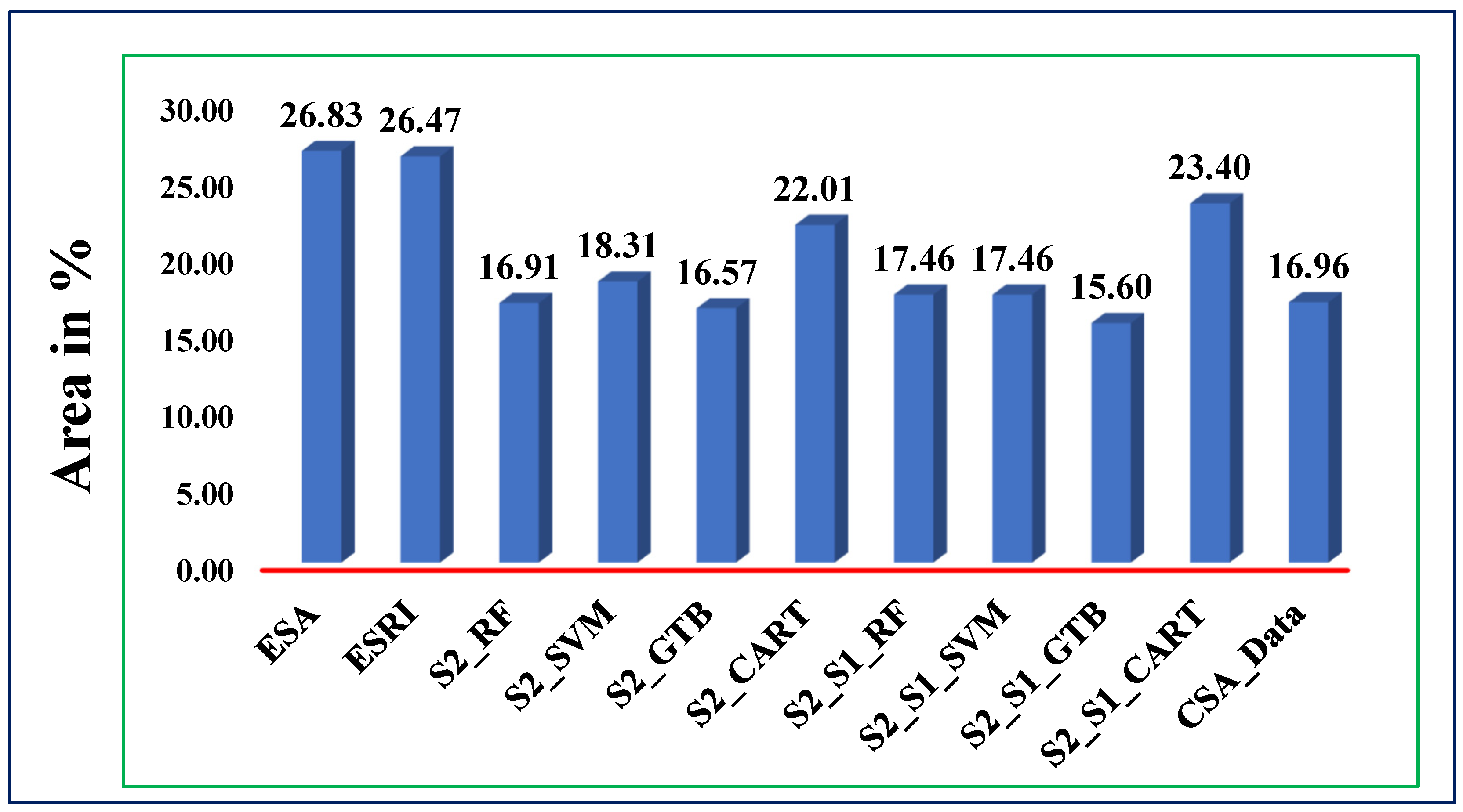
3.3. Acreage Estimation and Implications for Small Farm Holdings

The accurate estimation of acreage in small farm holdings has an important role in agricultural planning and management. The estimated areas for each LULC class provide valuable insights into the distribution of various crops within the study area. In this study, the area measurements were obtained for five land use land cover categories. The figure below illustrates the proportional distribution of land use land cover extracted from LULC maps generated through selected machine learning algorithms for classifications for optical image only (Figure 7 and Figure 8) and the combination of optical and radar (Figure 9 and Figure 10).
The Sentinel-2 classified image area results (Figure 7) showed that the area obtained for water classes was very close and similar across all four algorithms, indicating the robustness of the classification for this specific class. Similarly, the three algorithms, SVM, RF, and GTB, yielded fairly similar area measurements for agricultural land, vegetation, and bare land classes. Among these three algorithms, RF and GTB provided the very closest results.
From the findings, we observe that the RF and GTB algorithms achieved the same coverage for agricultural land, measuring 16.5%, when applied to optical imagery, while the CART algorithm exhibited the highest coverage for this class, about 22% of the total area (Figure 8). Conversely, the SVM, RF, and GTB classifiers demonstrated nearly similar coverage for vegetation accounts, 9.2%, 10.4%, and 10.5%, respectively, with the CART classifier having the least coverage, which measured 7.9%. Settlement coverage exhibited an inverse relationship with vegetation cover, with the CART classifier achieving the highest coverage (4.14%), followed by GTB (0.84%) and SVM (0.74%) classifiers, and the RF classifier exhibiting the lowest coverage measuring 0.64%. Notably, all classifiers achieved similar levels of coverage for water surface coverage (Figure 8).
By leveraging the complementary strengths of radar and optical data, acreage estimation becomes more robust, accounting for variations in crop phenology, crop structure, and soil conditions. To assess the spatial extent of different land use and land cover (LULC) classes, the areas of the S2-S1 maps of Figure 4 were generated. The results, presented in Figure 9 and the associated Figure 10, demonstrate significant variation in the areas of LULC classes across the models. Specifically, similar to Sentinel-2 alone classification, the CART model tends to overestimate agricultural land cover, measuring 75,574 ha (23.39%) of the total area, and built-up area, measuring 10,489 ha (3.24%) compared to the other models. On the other hand, it underestimates bare land and vegetation areas, measuring 207,243 ha (64.15%) and 26,949 ha (8.34%) in comparison to the other models. Interestingly, the SVM and RF models provide an equal estimate for agricultural land, measuring 17.45% of the total area, compared to the other three models.
Interestingly, the area of the agricultural land class by RF and SVM shows a strong correlation with the area of agriculture obtained from the central statistics data office, which is measured as 5,501,300.583 ha.
According to our findings, there are significant discrepancies in the acreage estimation obtained from the classification of Sentinel-2 alone (Figure 8) and the synergy of Sentinel-2 and Sentinel-1 data (Figure 10) for all land use and land cover classes. Among the four algorithms tested, the Support Vector Machine classifier demonstrated the smallest differences in acreage estimation between the two methods. The SVM algorithm displayed differences of less than 1% for each land use and land cover class between the two methods. This suggests that SVM are highly accurate and reliable in estimating acreage for agricultural land in small and fragmented farmlands.
Following SVM, the Gradient Boosting algorithm exhibited the second smallest variations in acreage estimation results. On the other hand, the Random Forest and Classification and Regression Tree classifiers displayed differences of up to 2% for certain land use and land cover categories. These findings highlight the effectiveness and robustness of the SVM classifier in identifying and mapping agricultural land in small and fragmented farmlands compared to the other classifiers utilized in this study.
However, the above approaches for area estimation are based on the summation of the area covered by the land cover map classification pixel, which does not adjust for classification errors in the map caused by class confusion [47,173,175]. Therefore, by incorporating the known area proportions of the map class in the stratified estimators of the overall and class-wise accuracies, the uncertainty and confidence interval in all classes (strata) can be computed.
Table 4 shows that the user’s accuracy of agricultural land mapping using Sentinel-2 alone varies between 75 and 88% depending on the classifier used. Conversely, when integrating Sentinel-2 and Sentinel-1 data, the user’s accuracy was between 83% and 92%. However, it is noted that the producer’s accuracy for agriculture was relatively low, ranging from 65 to 77%. This fact demonstrates that the maps failed to capture some portions of the agricultural area in the reference data. From the findings of this study, a high user accuracy coupled with a low producer accuracy for agricultural land implies that the majority of the land labeled as agricultural in the LULC map reflects the land cover for agriculture in the reference data.
As depicted in Table 4, considering the uncertainty in area estimation associated with pixel counting at the 95% confidence level, the true area of agricultural land may vary between 60,662 and 81,658 km2, covering 19–25% of the total surface in the study region.
To validate the accuracy of the results, we compared the area of the agricultural LULC class derived from each machine learning classifier in both classification results with data from Ethiopia statistics service as well as from ESA and ESRI Global land cover databases [176,177,178]. The results showed that SVM, RF, and GTB were found to be very close to the crop area data obtained from the country statistics data center. This indicates that these machine learning algorithms successfully captured and classified agricultural land use with high precision and accuracy. To further explain this, let us take a sample number.
The area of agricultural land derived from the country statistics data center is 16.96 percent of hectares. The machine learning classifiers, SVM, RF, and GTB, classified the agricultural land as approximately 17 percent of the total land coverage. This indicates a close match between the classifier results and the ground truth data. Furthermore, the area of the water surface from Global LULC is very similar to the area obtained in this study.
Furthermore, the area of agricultural land derived from machine learning algorithms was compared with agricultural land from the global Land Use and Land Cover (LULC) cover datasets of ESA and ESRI (Figure 11). To address this, the global LULC classifications were reclassified into five classes that were deemed to be highly important and relevant during the study period.
The result indicates that the area of agricultural land obtained from the global LULC datasets of ESA and ESRI is 26.5% and exhibited significant differences when compared to the results obtained using the machine learning algorithms, which involve 15–23% of the total coverage at the study area. These differences indicate variations in the classification accuracy and identification of agricultural land between the global datasets and the approach employed in this study. However, it was observed that the land use classes of built-up areas and water surfaces derived from the global LULC datasets demonstrated a closer agreement with the land cover classes obtained through the machine learning algorithms. This suggests that the classification of built-up areas and water surfaces in the global datasets aligns more closely with the machine learning results at a local level.
The findings also suggest that CART may not be the most suitable algorithm for the accurate estimation of agricultural areas in small farm areas. The overestimation observed in the CART results could be attributed to the complex nature of agricultural land and the limitations of the algorithms in handling such complexities.

4. Discussion

The main goals of this study were to assess the application of freely available high-resolution satellite imageries, particularly sentinel products, as well as the performance of the MLAs for detecting and differentiating agricultural areas at small and fragmented farmlands in developing countries.
Agricultural monitoring in sub-Saharan Africa is challenging due to inaccurate agricultural statistics and coarse data analysis [179,180]. However, the free availability of 10 m Sentinel-2 data and an advanced processing platform allows for efficient processing of high spatial resolution data, making crop area maps feasible [7,181,182]. The high spatial resolution satellite allows for fewer mixed pixels in these smallholder agricultural landscapes, resulting in mosaics of fields that are often heterogeneously mixed at lower resolution satellite data [183,184,185]. In this study, the high-resolution freely available sentinel data were evaluated, and the performances of commonly used MLAs were tested concerning the small and fragmented farmlands.
The classification based solely on Sentinel-2 imagery yielded reasonably accurate results, with overall accuracies ranging from 83.4% to 89.9% for the different machine learning algorithms utilized. The obtained accuracy metrics showed that all MLAs had highly acceptable accuracy values, with SVM having the highest values for overall accuracy and kappa coefficients. The overall accuracy of SVM in mapping agricultural land from the other four land covers consisted of an OA of 89.9% and kappa of 0.86. As a result, the agricultural and non-agricultural land cover could be distinguished. The result also indicates that most of the classes exceeded the 90% F-score criteria, with the class relating to vegetation cover achieving a value of 99%. In contrast, the CART-based classification for optical images of agricultural land cover resulted in the lowest F-score value (77%) due to incorrectly classifying pixels from the barren land class as agricultural and built-up. This omission error in the agriculture class is demonstrated by a user accuracy of 75% and a producer accuracy of 78% in the same class.
In this study, although the CART, in some cases, makes errors of omission by misclassifying water as barren land areas, bare land as built-up areas, and bare land as agriculture, the remaining classifiers demonstrate a relatively high level of confidence in differentiating different surface cover of the regions. In particular, RF and SVM delineate water with respective consumer and producer accuracies of 90%, 94%, and 93%, 98%, respectively.
The same study conducted by Ouma et al. [139] compares four machine learning algorithms, RF, GTB, SVM, and multilayer perceptron neural networks (MLP-ANN), for the classification of LULC and they found that SVM, RF, and GTB perform similarly to our findings. Furthermore, the finding of this study was aligned with the study conducted by Basheer [159], who evaluated the performances of SVM. Regarding RF, CART, and ML classification, they found that SVM outperforms the other approaches with an OA accuracy of 89%-94, depending on the data used. Similar to this study, they demonstrate the existence of a very slight difference between GTB and RF in the LCLU classification study using high-resolution data from RapidEye [186].
However, relying solely on optical imagery has limitations in accurately identifying land cover classes, particularly in areas with dense vegetation or cloud cover. This could explain the observed variations in classification accuracy among the different algorithms employed. Several recent studies have acknowledged the challenges associated with the misclassification of land cover classes when using only optical data. The combination of SAR and multispectral data offers a more comprehensive approach to land cover mapping and can lead to improved results [187].
Therefore, in this study, integrating Sentinel-1 radar data with Sentinel-2 optical data, a significant improvement in classification accuracy was achieved across all machine learning algorithms applied. The overall accuracies ranged from 87.6% to 93.7%, indicating the significance of combining radar and optical data sources for accurate agricultural mapping in small farmlands. The result shows that SVM yields the highest OA at 94% and Ka at 91%, respectively (Table 3). Similarly, different studies demonstrate the highest OA accuracy of classification by integration of optical and radar datasets [188,189].
The results of the study indicate that the integration of Sentinel-1 and Sentinel-2 satellites resulted in an improvement in the overall accuracy of the classification by approximately 3–4.5%. This finding was confirmed by the studies on the improvement in accuracy of the classification by the integration of SAR to optical by >2.5% compared to that obtained using only optical data [175,190]. Furthermore, the previous study has shown that combining Synthetic Aperture Radar (SAR)-optical data improves the classification accuracy of Machine Learning Algorithms (MLAs) by 4%. This improvement was especially noticeable in areas with diverse landscapes and weather conditions that make remote sensing data collection difficult. Similarly, the investigation by Khan et al. [170] confirmed that the addition of VV and VH into Sentinel-2 data increased the kappa coefficient from 75% to 82%.
Our result is aligned with the study that demonstrates that adding the radar-derived index into optical bands increases the accuracy of classification [191]. Furthermore, the Studies conducted by Nicolau et al. [192] and De Luca et al. [175] emphasize the complementary nature of SAR and optical imagery, suggesting that their integration can provide a more comprehensive understanding of land cover characteristics.
The finding indicates that good overall accuracy was achieved by the integrated optical and SAR datasets, represented by a mean F-score equal to 94.28%, which is in line with the outcomes obtained from other studies where the combination of optical and SAR data was used.
This result was confirmed with the study conducted to evaluate the performances of SVM, RF, and K-NN. They found that the SVM technique resulted in the highest OA (88.75) and ka (0.86) to classify LULC by radar and optical integrated dataset and they concluded that the overall accuracy of the integrated dataset is higher than the single image [193]. According to recent reviews, support vector machines (SVM) and random forest (RF) are the most popular machine learning algorithms for classification, with comparable high accuracy [66,146,194], but the conclusion on which classifier performs better in LULC classification is unclear. According to the findings, some classes are wrongly identified, and it was difficult to differentiate between built-up, barren land, and vegetation classes by optical scene compared to the synergistic of optical with radar sceneries due to mixed pixels in a very small plot.
Crop acreage is one of the most important pieces of information needed to quantify food production at the regional or country level, which will be used for the implementation of sustainable agricultural management systems and monitoring the progress toward the SDGs [195]. The findings of this study highlight the importance of carefully selecting the appropriate machine learning algorithm for accurate estimation of area. There is variability in the classification of land use and land cover (LULC) classes between different classifiers [131], as demonstrated in Figure 8 and Figure 10. This discrepancy in LULC classes can be attributed to variations in parameter optimization within the algorithms employed [159]. Furthermore, the differences in area estimation among the classifiers may be attributed to the inherent characteristics and biases of each algorithm and the size of the parcel. Various studies have found that the areas of different land use and land cover (LULC) classes vary depending on the classification technique [121,160,196]. This study also observed variations in the results of four classifiers, where the area under each LULC class of one classifier did not exactly match the area under the same class of another classifier.
However, the map provides an area estimate for agricultural land without considering the uncertainty in pixel counts. Subsequently, through the creation of an error matrix, the error-adjusted/unbiased area of agricultural land, along with the confidence interval, was computed. The result provides additional information into area estimation, which significantly deviates from results obtained solely through pixel counting methodologies.
The LULC classification map provides a single area estimate for each land cover class without a confidence interval. In this study, an error matrix was generated from the class strata sample pixel counts. Subsequently, accuracy assessments and confidence intervals were derived. The results, presented in Table 4, show that the overall accuracy metric using this method aligns with those obtained directly from the pixel-based confusion matrix, with SVM having the maximum OA of 92%. However, slight differences are observed in users’ accuracy and significant variation in producer accuracy with different machine learning algorithms. These findings are consistent with previous studies that have demonstrated there is more variation in the producer’s accuracies than in the user’s accuracies [145,197].
In this instance, the mapped area of agricultural land ranges from 15.6% to 23.4% ha for the integrated dataset and from 16.6% to 22% ha for Sentinel-2-based classification. However, the stratified error-adjusted area estimate for agricultural land is approximately 18.7% to 25.2% for the integrated dataset and 21% to 24.6% for optical image only (Table 4). This disparity can be attributed to the error matrix, which indicates that some of the proportion of the area of agricultural land is omitted from the map. These results are in line with other similar studies that have also demonstrated the improved accuracy of area estimation by considering the uncertainty in the error matrix and confidence interval [198,199,200].
Furthermore, complicating matters further, the research area is situated in a developing country characterized by unmodernized farming systems with small, fragmented farm sizes. The small size of farmlands coupled with the cultivation of different crops on these diminutive plots poses challenges in identifying and delineating agricultural areas [36]. Additionally, the presence of various types of grass used for grazing and boundary marking further hinders the precise determination of agricultural land and its extent. In such cases, remote sensing technology encounters difficulties in performing accurate LULC classification. Another issue faced during the study was the existence of pastureland between crops. Pastureland typically has a different spectral signature compared to crops, and its presence further complicates the classification process. For example, in some areas where pastureland existed between maize fields, the classification algorithm struggled to differentiate between the two land cover types accurately. This led to misclassifications and reduced accuracy in those specific areas.

5. Conclusions

The primary objective of this study was to evaluate the suitability of Sentinel-2 and Sentinel-1 products for the analysis of agricultural land within a small and fragmented farm region during the Meher season of the year 2020/2021. The application of freely available multi-source imagery for agricultural mapping in small-scale farmlands is important for many developing countries that face budget constraints in acquiring high-resolution data. The results reveal the potential of freely available sentinel products, especially when integrating Sentinel-1 and Sentinel-2 data for mapping agricultural areas and estimating acreage within small farmlands in developing countries. The integration of Sentinel-1 data with Sentinel-2 data, along with the use of advanced classification algorithms, can significantly improve the accuracy of agricultural mapping and acreage estimation. When the findings from Sentinel-2 alone were compared to the synergy of Sentinel-2 and Sentinel-1 imagery, the synergistic dataset produced the highest OA and Ka accuracy results for agricultural mapping and acreage estimation on small, fragmented farmlands and heterogeneous cropping parcels.
In terms of accuracy comparison, the findings of this analysis consistently demonstrate that SVM, RF, and GTB yield comparable high accuracies. But SVM outperform with a very slight difference in terms of overall accuracy (OA) and kappa coefficient. It is believed that the acquisition of an accurate agricultural map with an estimate of accuracy of more than 90% has significance for improving further monitoring and analysis of agricultural land in a small and fragmented farmland region.
In terms of acreage estimation, two approaches were employed: direct calculation from pixel values and stratified sampling using LULC map classes as strata. Notably, the integrated Sentinel-2 and Sentinel-1 approach yielded promising results in both methods. The application of stratified sampling for unbiased area estimation, supported by a 95% confidence interval, revealed that the integrated approach outperformed the Sentinel-2-alone classification, producing results closely comparable to the ground truth data.
These outcomes demonstrate the remarkable potential of freely accessible multi-source remotely sensed data in agricultural mapping and acreage estimation operations in small farm holdings. They also further demonstrate the significant capability of such data in supporting the monitoring and management of agricultural resources in small-scale farmlands within developing countries.

Author Contributions

Conceptualization: T.E.M.; Methodology: T.E.M. and P.G.; Formal analysis and investigation: T.E.M., P.G., G.T.A. and L.T.D.; Writing-original draft preparation: T.E.M.; Writing-review and editing: T.E.M., P.G., L.T.D. and G.T.A. All authors have read and agreed to the published version of the manuscript.

Funding

This research received no external funding.

Data Availability Statement

All the sentinel products and the GEE code used to process the S2 and S1 in this study are available in the GEE JavaScript environment. The Auxilary data supporting this study’s findings are available from the corresponding author upon reasonable request.

Acknowledgments

The authors gratefully thank the anonymous reviewers and the editors whose valuable comments and suggestions have helped improve the quality of this article.

Conflicts of Interest

The authors declare no conflict of interest.

References

  1. Akinyemi, F.O.; Ifejika Speranza, C. Agricultural landscape change impact on the quality of land: An African continent-wide assessment in gained and displaced agricultural lands. Int. J. Appl. Earth Obs. Geoinf. 2022, 106, 102644. [Google Scholar] [CrossRef]
  2. Baptista, D.; Miguel Salgado, F.; Fayad, M.; Kemoe, D.; Lanci, L.; Mitra, L.S.; Muehlschlegel, P.; Okou, T.S.; Spray, C.; Tuitoek, K.J.; et al. Climate change and SSA’s intensified food insecurity. Int. Monet. Fund 2022, 2022, 1–48. [Google Scholar]
  3. Choi, Y.W.; Eltahir, E.A.B. Near-term climate change impacts on food crops productivity in East Africa. Theor. Appl. Climatol. 2023, 152, 843–860. [Google Scholar] [CrossRef]
  4. Mechiche-Alami, A.; Abdi, A.M. Agricultural productivity in relation to climate and cropland management in West Africa. Sci. Rep. 2020, 10, 3393. [Google Scholar] [CrossRef]
  5. Giller, K.E.; Delaune, T.; Silva, J.V.; van Wijk, M.; Hammond, J.; Descheemaeker, K.; van de Ven, G.; Schut, A.G.T.; Taulya, G.; Chikowo, R.; et al. Small farms and development in sub-Saharan Africa: Farming for food, for income or for lack of better options? Food Secur. 2021, 13, 1431–1454. [Google Scholar] [CrossRef]
  6. Jayne, T.S.; Wineman, A.; Chamberlin, J.; Muyanga, M.; Yeboah, F.K. Changing Farm Size Distributions and Agricultural Transformation in Sub-Saharan Africa. Annu. Rev. Resour. Econ. 2022, 14, 109–130. [Google Scholar] [CrossRef]
  7. Peterson, S.; Husak, G. Crop Area Mapping in Southern and Central Malawi With Google Earth Engine. Front. Clim. 2021, 3, 693653. [Google Scholar] [CrossRef]
  8. Yigezu Wendimu, G. The challenges and prospects of Ethiopian agriculture. Cogent Food Agric. 2021, 7, 1923619. [Google Scholar] [CrossRef]
  9. Zerssa, G.; Feyssa, D.; Kim, D.G.; Eichler-Löbermann, B. Challenges of smallholder farming in Ethiopia and opportunities by adopting climate-smart agriculture. Agriculture 2021, 11, 192. [Google Scholar] [CrossRef]
  10. Headey, D.; Dereje, M.; Taffesse, A.S. Land constraints and agricultural intensification in Ethiopia: A village-level analysis of high-potential areas. Food Policy 2014, 48, 129–141. [Google Scholar] [CrossRef]
  11. Seyoum Taffesse, A.; Dorosh, P.; Gemessa, S.A. Crop production in Ethiopia: Regional patterns and trends. Food Agric. Ethiop. Prog. Policy Chall. 2013, 9780812208, 53–83. [Google Scholar] [CrossRef]
  12. Mashaba-Munghemezulu, Z.; Chirima, G.J.; Munghemezulu, C. Mapping smallholder maize farms using multi-temporal sentinel-1 data in support of the sustainable development goals. Remote Sens. 2021, 13, 1666. [Google Scholar] [CrossRef]
  13. Duncan, J.M.A.; Dash, J.; Atkinson, P.M. The potential of satellite-observed crop phenology to enhance yield gap assessments in smallholder landscapes. Front. Environ. Sci. 2015, 3, 56. [Google Scholar] [CrossRef]
  14. Bégué, A.; Arvor, D.; Lelong, C.; Vintrou, E. Agricultural Systems Studies using Remote Sensing to cite this version: HAL Id: Hal-02098284. Hal 2019. Available online: https://hal.science/hal-02098284 (accessed on 29 January 2024).
  15. Neigh, C.S.R.; Carroll, M.L.; Wooten, M.R.; McCarty, J.L.; Powell, B.F.; Husak, G.J.; Enenkel, M.; Hain, C.R. Smallholder crop area mapped with wall-to-wall WorldView sub-meter panchromatic image texture: A test case for Tigray, Ethiopia. Remote Sens. Environ. 2018, 212, 8–20. [Google Scholar] [CrossRef]
  16. Warner, J.M.; Mann, M.L. Agricultural Impacts of the 2015/2016 Drought in Ethiopia Using High-Resolution Data Fusion Methodologies. Handb. Clim. Chang. Resil. 2019, 2, 869–894. [Google Scholar] [CrossRef]
  17. Abdul-Jabbar, T.S.; Ziboon, A.T.; Albayati, M.M. Crop yield estimation using different remote sensing data: Literature review. IOP Conf. Ser. Earth Environ. Sci. 2023, 1129, 012004. [Google Scholar] [CrossRef]
  18. Hudait, M.; Patel, P.P. Crop-type mapping and acreage estimation in smallholding plots using Sentinel-2 images and machine learning algorithms: Some comparisons. Egypt. J. Remote Sens. Space Sci. 2022, 25, 147–156. [Google Scholar] [CrossRef]
  19. Saini, R.; Ghosh, S.K. Crop classification in a heterogeneous agricultural environment using ensemble classifiers and single-date Sentinel-2A imagery. Geocarto Int. 2021, 36, 2141–2159. [Google Scholar] [CrossRef]
  20. Waldner, F.; Hansen, M.C.; Potapov, P.V.; Löw, F.; Newby, T.; Ferreira, S.; Defourny, P. National-scale cropland mapping based on spectral-temporal features and outdated land cover information. PLoS ONE 2017, 12, e0181911. [Google Scholar] [CrossRef]
  21. Sun, C.; Bian, Y.; Zhou, T.; Pan, J. Using of multi-source and multi-temporal remote sensing data improves crop-type mapping in the subtropical agriculture region. Sensors 2019, 19, 2401. [Google Scholar] [CrossRef] [PubMed]
  22. Xie, G.; Niculescu, S. Mapping Crop Types Using Sentinel-2 Data Machine Learning and Monitoring Crop Phenology with Sentinel-1 Backscatter Time Series in Pays de Brest, Brittany, France. Remote Sens. 2022, 14, 4437. [Google Scholar] [CrossRef]
  23. Santaga, F.S.; Agnelli, A.; Leccese, A.; Vizzari, M. Using sentinel-2 for simplifying soil sampling and mapping: Two case studies in Umbria, Italy. Remote Sens. 2021, 13, 3379. [Google Scholar] [CrossRef]
  24. Sarteshnizi, R.E.; Vayghan, S.S.; Jazirian, I. Estimation of Soil Moisture Using Sentinel-1 and Sentinel-2 Images. ISPRS Ann. Photogramm. Remote Sens. Spat. Inf. Sci. 2023, 10, 137–142. [Google Scholar] [CrossRef]
  25. Rukhovich, D.I.; Koroleva, P.V.; Rukhovich, A.D.; Komissarov, M.A. Updating of the Archival Large-Scale Soil Map Based on the Multitemporal Spectral Characteristics of the Bare Soil Surface Landsat Scenes. Remote Sens. 2023, 15, 4491. [Google Scholar] [CrossRef]
  26. Ofori-Ampofo, S.; Pelletier, C.; Lang, S. Crop type mapping from optical and radar time series using attention-based deep learning. Remote Sens. 2021, 13, 4668. [Google Scholar] [CrossRef]
  27. Chang, Z.; Li, H.; Chen, D.; Liu, Y.; Zou, C.; Chen, J.; Han, W.; Liu, S.; Zhang, N. Crop Type Identification Using High-Resolution Remote Sensing Images Based on an Improved DeepLabV3+ Network. Remote Sens. 2023, 15, 5088. [Google Scholar] [CrossRef]
  28. Hosseini, M.; Becker-Reshef, I.; Sahajpal, R.; Fontana, L.; Lafluf, P.; Leale, G.; Puricelli, E.; Varela, M.; Justice, C. Crop yield prediction using integration of polarimteric synthetic aperture radar and optical data. In Proceedings of the 2020 IEEE India Geoscience and Remote Sensing Symposium (InGARSS), Ahmedabad, India, 1–4 December 2020; pp. 17–20. [Google Scholar] [CrossRef]
  29. Ali, A.M.; Abouelghar, M.; Belal, A.A.; Saleh, N.; Yones, M.; Selim, A.I.; Amin, M.E.S.; Elwesemy, A.; Kucher, D.E.; Maginan, S.; et al. Crop Yield Prediction Using Multi Sensors Remote Sensing (Review Article). Egypt. J. Remote Sens. Sp. Sci. 2022, 25, 711–716. [Google Scholar] [CrossRef]
  30. Ranjan, A.K.; Parida, B.R. Predicting paddy yield at spatial scale using optical and Synthetic Aperture Radar (SAR) based satellite data in conjunction with field-based Crop Cutting Experiment (CCE) data. Int. J. Remote Sens. 2021, 42, 2046–2071. [Google Scholar] [CrossRef]
  31. Borra, S.; Thanki, R.; Dey, N. Satellite Image Analysis: Clustering and Classification; Springer: Singapore, 2019; ISBN 978-981-13-6423-5. [Google Scholar]
  32. Tarasenkov, M.V.; Belov, V.V.; Engel, M.V.; Zimovaya, A.V.; Zonov, M.N.; Bogdanova, A.S. Algorithm for the Reconstruction of the Ground Surface Reflectance in the Visible and Near IR Ranges from MODIS Satellite Data with Allowance for the Influence of Ground Surface Inhomogeneity on the Adjacency Effect and of Multiple Radiation Reflection. Remote Sens. 2023, 15, 2655. [Google Scholar] [CrossRef]
  33. Ustin, S.L.; Middleton, E.M. Current and near-term advances in Earth observation for ecological applications. Ecol. Process. 2021, 10, 1. [Google Scholar] [CrossRef]
  34. Yu, X.; Lu, D.; Jiang, X.; Li, G.; Chen, Y.; Li, D.; Chen, E. Examining the roles of spectral, spatial, and topographic features in improving land-cover and forest classifications in a subtropical region. Remote Sens. 2020, 12, 2907. [Google Scholar] [CrossRef]
  35. Zhao, P.; Lu, D.; Wang, G.; Wu, C.; Huang, Y.; Yu, S. Examining spectral reflectance saturation in landsat imagery and corresponding solutions to improve forest aboveground biomass estimation. Remote Sens. 2016, 8, 469. [Google Scholar] [CrossRef]
  36. Persello, C.; Tolpekin, V.A.; Bergado, J.R.; de By, R.A. Delineation of agricultural fields in smallholder farms from satellite images using fully convolutional networks and combinatorial grouping. Remote Sens. Environ. 2019, 231, 111253. [Google Scholar] [CrossRef] [PubMed]
  37. Cucho-Padin, G.; Loayza, H.; Palacios, S.; Balcazar, M.; Carbajal, M.; Quiroz, R. Development of low-cost remote sensing tools and methods for supporting smallholder agriculture. Appl. Geomat. 2020, 12, 247–263. [Google Scholar] [CrossRef]
  38. Sishodia, R.P.; Ray, R.L.; Singh, S.K. Applications of remote sensing in precision agriculture: A review. Remote Sens. 2020, 12, 3136. [Google Scholar] [CrossRef]
  39. Waleed, M.; Mubeen, M.; Ahmad, A.; Habib-ur-Rahman, M.; Amin, A.; Farid, H.U.; Hussain, S.; Ali, M.; Qaisrani, S.A.; Nasim, W.; et al. Evaluating the efficiency of coarser to finer resolution multispectral satellites in mapping paddy rice fields using GEE implementation. Sci. Rep. 2022, 12, 13210. [Google Scholar] [CrossRef]
  40. Chaves, M.E.D.; Picoli, M.C.A.; Sanches, I.D. Recent applications of Landsat 8/OLI and Sentinel-2/MSI for land use and land cover mapping: A systematic review. Remote Sens. 2020, 12, 3062. [Google Scholar] [CrossRef]
  41. Segarra, J.; Buchaillot, M.L.; Araus, J.L.; Kefauver, S.C. Remote sensing for precision agriculture: Sentinel-2 improved features and applications. Agronomy 2020, 10, 641. [Google Scholar] [CrossRef]
  42. Ma, L.; Liu, Y.; Zhang, X.; Ye, Y.; Yin, G.; Johnson, B.A. Deep learning in remote sensing applications: A meta-analysis and review. ISPRS J. Photogramm. Remote Sens. 2019, 152, 166–177. [Google Scholar] [CrossRef]
  43. Orynbaikyzy, A.; Gessner, U.; Mack, B.; Conrad, C. Crop type classification using fusion of sentinel-1 and sentinel-2 data: Assessing the impact of feature selection, optical data availability, and parcel sizes on the accuracies. Remote Sens. 2020, 12, 2779. [Google Scholar] [CrossRef]
  44. Van Tricht, K.; Gobin, A.; Gilliams, S.; Piccard, I. Synergistic use of radar sentinel-1 and optical sentinel-2 imagery for crop mapping: A case study for Belgium. Remote Sens. 2018, 10, 1642. [Google Scholar] [CrossRef]
  45. Niculescu, S.; Lardeux, C.; Hanganu, J. Synergy between Sentinel-1 radar time series and Sentinel-2 optical for the mapping of restored areas in Danube delta. Proc. ICA 2018, 1, 82. [Google Scholar] [CrossRef]
  46. Huang, D.; Tang, Y.; Wang, Q. An Image Fusion Method of SAR and Multispectral Images Based on Non-Subsampled Shearlet Transform and Activity Measure. Sensors 2022, 22, 7055. [Google Scholar] [CrossRef]
  47. Ienco, D.; Interdonato, R.; Gaetano, R.; Ho Tong Minh, D. Combining Sentinel-1 and Sentinel-2 Satellite Image Time Series for land cover mapping via a multi-source deep learning architecture. ISPRS J. Photogramm. Remote Sens. 2019, 158, 11–22. [Google Scholar] [CrossRef]
  48. Gargiulo, M.; Dell’aglio, D.A.G.; Iodice, A.; Riccio, D.; Ruello, G. Integration of sentinel-1 and sentinel-2 data for land cover mapping using w-net. Sensors 2020, 20, 2969. [Google Scholar] [CrossRef] [PubMed]
  49. Chapa, F.; Hariharan, S.; Hack, J. A new approach to high-resolution urban land use classification using open access software and true color satellite images. Sustainability 2019, 11, 5266. [Google Scholar] [CrossRef]
  50. Géant, C.B.; Gustave, M.N.; Schmitz, S. Mapping small inland wetlands in the South-Kivu province by integrating optical and SAR data with statistical models for accurate distribution assessment. Sci. Rep. 2023, 13, 17626. [Google Scholar] [CrossRef] [PubMed]
  51. Joshi, N.; Baumann, M.; Ehammer, A.; Fensholt, R.; Grogan, K.; Hostert, P.; Jepsen, M.R.; Kuemmerle, T.; Meyfroidt, P.; Mitchard, E.T.A.; et al. A review of the application of optical and radar remote sensing data fusion to land use mapping and monitoring. Remote Sens. 2016, 8, 70. [Google Scholar] [CrossRef]
  52. Qin, R.; Liu, T. A Review of Landcover Classification with Very-High Resolution Remotely Sensed Optical Images—Analysis Unit, Model Scalability and Transferability. Remote Sens. 2022, 14, 646. [Google Scholar] [CrossRef]
  53. Latif, R.M.A.; He, J.; Umer, M. Mapping Cropland Extent in Pakistan Using Machine Learning Algorithms on Google Earth Engine Cloud Computing Framework. ISPRS Int. J. Geo-Inf. 2023, 12, 81. [Google Scholar] [CrossRef]
  54. Pech-May, F.; Aquino-Santos, R.; Rios-Toledo, G.; Posadas-Durán, J.P.F. Mapping of Land Cover with Optical Images, Supervised Algorithms, and Google Earth Engine. Sensors 2022, 22, 4729. [Google Scholar] [CrossRef]
  55. Bolfe, É.L.; Parreiras, T.C.; da Silva, L.A.P.; Sano, E.E.; Bettiol, G.M.; Victoria, D.d.C.; Sanches, I.D.; Vicente, L.E. Mapping Agricultural Intensification in the Brazilian Savanna: A Machine Learning Approach Using Harmonized Data from Landsat Sentinel-2. ISPRS Int. J. Geo-Inf. 2023, 12, 263. [Google Scholar] [CrossRef]
  56. Akhavan, Z.; Hasanlou, M.; Hosseini, M. A Comparison of Tree-Based Regression Models for Soil Moisture Estimation Using Sar Data. ISPRS Ann. Photogramm. Remote Sens. Spat. Inf. Sci. 2023, 10, 37–42. [Google Scholar] [CrossRef]
  57. Tufail, R.; Ahmad, A.; Javed, M.A.; Ahmad, S.R. A machine learning approach for accurate crop type mapping using combined SAR and optical time series data. Adv. Space Res. 2022, 69, 331–346. [Google Scholar] [CrossRef]
  58. Akbari, E.; Boloorani, A.D.; Samany, N.N.; Hamzeh, S.; Soufizadeh, S.; Pignatti, S. Crop mapping using random forest and particle swarm optimization based on multi-temporal sentinel-2. Remote Sens. 2020, 12, 1449. [Google Scholar] [CrossRef]
  59. Kok, Z.H.; Mohamed Shariff, A.R.; Alfatni, M.S.M.; Khairunniza-Bejo, S. Support Vector Machine in Precision Agriculture: A review. Comput. Electron. Agric. 2021, 191, 106546. [Google Scholar] [CrossRef]
  60. Zheng, B.; Myint, S.W.; Thenkabail, P.S.; Aggarwal, R.M. A support vector machine to identify irrigated crop types using time-series Landsat NDVI data. Int. J. Appl. Earth Obs. Geoinf. 2015, 34, 103–112. [Google Scholar] [CrossRef]
  61. Camargo, F.F.; Sano, E.E.; Almeida, C.M.; Mura, J.C.; Almeida, T. A comparative assessment of machine-learning techniques for land use and land cover classification of the Brazilian tropical savanna using ALOS-2/PALSAR-2 polarimetric images. Remote Sens. 2019, 11, 1600. [Google Scholar] [CrossRef]
  62. Jamali, A. Evaluation and comparison of eight machine learning models in land use/land cover mapping using Landsat 8 OLI: A case study of the northern region of Iran. SN Appl. Sci. 2019, 1, 1448. [Google Scholar] [CrossRef]
  63. Mahmoud, R.; Hassanin, M.; Al Feel, H.; Badry, R.M. Machine Learning-Based Land Use and Land Cover Mapping Using Multi-Spectral Satellite Imagery: A Case Study in Egypt. Sustainability 2023, 15, 9467. [Google Scholar] [CrossRef]
  64. Oo, T.K.; Arunrat, N.; Sereenonchai, S.; Ussawarujikulchai, A.; Chareonwong, U.; Nutmagul, W. Comparing Four Machine Learning Algorithms for Land Cover Classification in Gold Mining: A Case Study of Kyaukpahto Gold Mine, Northern Myanmar. Sustainability 2022, 14, 10754. [Google Scholar] [CrossRef]
  65. Razafinimaro, A.; Hajalalaina, A.R.; Rakotonirainy, H.; Zafimarina, R. Land cover classification based optical satellite images using machine learning algorithms. Int. J. Adv. Intell. Inform. 2022, 8, 362–380. [Google Scholar] [CrossRef]
  66. Adugna, T.; Xu, W.; Fan, J. Comparison of Random Forest and Support Vector Machine Classifiers for Regional Land Cover Mapping Using Coarse Resolution FY-3C Images. Remote Sens. 2022, 14, 574. [Google Scholar] [CrossRef]
  67. Dash, P.; Sanders, S.L.; Parajuli, P.; Ouyang, Y. Improving the Accuracy of Land Use and Land Cover Classification of Landsat Data in an Agricultural Watershed. Remote Sens. 2023, 15, 4020. [Google Scholar] [CrossRef]
  68. Burke, M.; Lobell, D.B. Satellite-based assessment of yield variation and its determinants in smallholder African systems. Proc. Natl. Acad. Sci. USA 2017, 114, 2189–2194. [Google Scholar] [CrossRef] [PubMed]
  69. Kpienbaareh, D.; Sun, X.; Wang, J.; Luginaah, I.; Kerr, R.B.; Lupafya, E.; Dakishoni, L. Crop type and land cover mapping in northern malawi using the integration of sentinel-1, sentinel-2, and planetscope satellite data. Remote Sens. 2021, 13, 700. [Google Scholar] [CrossRef]
  70. Solórzano, J.V.; Mas, J.F.; Gao, Y.; Gallardo-Cruz, J.A. Land use land cover classification with U-net: Advantages of combining sentinel-1 and sentinel-2 imagery. Remote Sens. 2021, 13, 3600. [Google Scholar] [CrossRef]
  71. Li, M.; Stein, A. Mapping land use from high resolution satellite images by exploiting the spatial arrangement of land cover objects. Remote Sens. 2020, 12, 4158. [Google Scholar] [CrossRef]
  72. Whyte, A.; Ferentinos, K.P.; Petropoulos, G.P. A new synergistic approach for monitoring wetlands using Sentinels -1 and 2 data with object-based machine learning algorithms. Environ. Model. Softw. 2018, 104, 40–54. [Google Scholar] [CrossRef]
  73. Zhang, L.; Hu, Q.; Tang, Z. Using Sentinel-2 Imagery and Machine Learning Algorithms to Assess the Inundation Status of Nebraska Conservation Easements during 2018–2021. Remote Sens. 2022, 14, 4382. [Google Scholar] [CrossRef]
  74. Ashton, R.A.; Kefyalew, T.; Tesfaye, G.; Pullan, R.L.; Yadeta, D.; Reithinger, R.; Kolaczinski, J.H.; Brooker, S. School-based surveys of malaria in Oromia Regional State, Ethiopia: A rapid survey method for malaria in low transmission settings. Malar. J. 2011, 10, 25. [Google Scholar] [CrossRef]
  75. Adugna, A. Demography and Health Aynalem Adugna July, 2014. 2014. Available online: http://www.ethiodemographyandhealth.org/ (accessed on 29 January 2024).
  76. Iiyama, M.; Derero, A.; Kelemu, K.; Muthuri, C.; Kinuthia, R.; Ayenkulu, E.; Kiptot, E.; Hadgu, K.; Mowo, J.; Sinclair, F.L. Understanding patterns of tree adoption on farms in semi-arid and sub-humid Ethiopia. Agrofor. Syst. 2017, 91, 271–293. [Google Scholar] [CrossRef]
  77. Tilahun, M.; Tefesa, M.; Girma, T.; Milkiyas, M.; Tamirat, H. Climate Change Indicators Trace for Identification of Climate Change Climatology & Weather Forecasting Climate Change Indicators Trace for Identification of Climate Change Vulnerability in Salale Zone, Oromia Region, Ethiopia. J. Climatol. Weather. Forecast. 2021, 9, 298. [Google Scholar]
  78. Brychkova, G.; Kekae, K.; McKeown, P.C.; Hanson, J.; Jones, C.S.; Thornton, P.; Spillane, C. Climate change and land-use change impacts on future availability of forage grass species for Ethiopian dairy systems. Sci. Rep. 2022, 12, 20512. [Google Scholar] [CrossRef] [PubMed]
  79. Central Statistical Agency (CSA). The Federa Democratic Republic of Ethiopia Report on Area and Production of Majr Crops. Addis Ababa Ethiop. 2020. [Google Scholar]
  80. Li, H.; Wang, C.; Zhong, C.; Zhang, Z.; Liu, Q. Mapping typical urban LULC from landsat imagery without training samples or self-defined parameters. Remote Sens. 2017, 9, 700. [Google Scholar] [CrossRef]
  81. Dobrinić, D.; Gašparović, M.; Medak, D. Sentinel-1 and 2 time-series for vegetation mapping using random forest classification: A case study of northern croatia. Remote Sens. 2021, 13, 2321. [Google Scholar] [CrossRef]
  82. Orieschnig, C.A.; Belaud, G.; Venot, J.P.; Massuel, S.; Ogilvie, A. Input imagery, classifiers, and cloud computing: Insights from multi-temporal LULC mapping in the Cambodian Mekong Delta. Eur. J. Remote Sens. 2021, 54, 398–416. [Google Scholar] [CrossRef]
  83. Saad El Imanni, H.; El Harti, A.; Hssaisoune, M.; Velastegui-Montoya, A.; Elbouzidi, A.; Addi, M.; El Iysaouy, L.; El Hachimi, J. Rapid and Automated Approach for Early Crop Mapping Using Sentinel-1 and Sentinel-2 on Google Earth Engine; A Case of a Highly Heterogeneous and Fragmented Agricultural Region. J. Imaging 2022, 8, 316. [Google Scholar] [CrossRef]
  84. Felegari, S.; Sharifi, A.; Moravej, K.; Amin, M.; Golchin, A.; Muzirafuti, A.; Tariq, A.; Zhao, N. Integration of sentinel 1 and sentinel 2 satellite images for crop mapping. Appl. Sci. 2021, 11, 10104. [Google Scholar] [CrossRef]
  85. Drusch, M.; Del Bello, U.; Carlier, S.; Colin, O.; Fernandez, V.; Gascon, F.; Hoersch, B.; Isola, C.; Laberinti, P.; Martimort, P.; et al. Sentinel-2: ESA’s Optical High-Resolution Mission for GMES Operational Services. Remote Sens. Environ. 2012, 120, 25–36. [Google Scholar] [CrossRef]
  86. Gascon, F.; Bouzinac, C.; Thépaut, O.; Jung, M.; Francesconi, B.; Louis, J.; Lonjou, V.; Lafrance, B.; Massera, S.; Gaudel-Vacaresse, A.; et al. Copernicus Sentinel-2A calibration and products validation status. Remote Sens. 2017, 9, 584. [Google Scholar] [CrossRef]
  87. Djamai, N.; Fernandes, R. Comparison of SNAP-derived Sentinel-2A L2A product to ESA product over Europe. Remote Sens. 2018, 10, 926. [Google Scholar] [CrossRef]
  88. Torres, R.; Snoeij, P.; Geudtner, D.; Bibby, D.; Davidson, M.; Attema, E.; Potin, P.; Rommen, B.; Floury, N.; Brown, M.; et al. GMES Sentinel-1 mission. Remote Sens. Environ. 2012, 120, 9–24. [Google Scholar] [CrossRef]
  89. Filipponi, F.; Smiraglia, D.; Agrillo, E. Earth Observation for Phenological Metrics (EO4PM): Temporal Discriminant to Characterize Forest Ecosystems. Remote Sens. 2022, 14, 721. [Google Scholar] [CrossRef]
  90. Schmidt, K.; Schwerdt, M.; Hajduch, G.; Vincent, P.; Recchia, A.; Pinheiro, M. Radiometric Re-Compensation of Sentinel-1 SAR Data Products for Artificial Biases due to Antenna Pattern Changes. Remote Sens. 2023, 15, 1377. [Google Scholar] [CrossRef]
  91. Mullissa, A.; Vollrath, A.; Odongo-Braun, C.; Slagter, B.; Balling, J.; Gou, Y.; Gorelick, N.; Reiche, J. Sentinel-1 sar backscatter analysis ready data preparation in google earth engine. Remote Sens. 2021, 13, 1954. [Google Scholar] [CrossRef]
  92. Laine, J. Crop Identification with Sentinel-2 Satellite Imagery in Finland. Master’s Thesis, Aalto University, Espoo, Finland, 2018; pp. 1–84. [Google Scholar]
  93. Sun, G.; Li, Z.; Zhang, A.; Wang, X.; Ding, S.; Jia, X.; Li, J.; Liu, Q. High-resolution and Multitemporal Impervious Surface Mapping in the Lancang-Mekong Basin with Google Earth Engine. Earth Syst. Sci. Data Discuss. 2022, 1–29. [Google Scholar] [CrossRef]
  94. Huang, C.; Zhang, C.; He, Y.; Liu, Q.; Li, H.; Su, F.; Liu, G.; Bridhikitti, A. Land cover mapping in cloud-prone tropical areas using Sentinel-2 data: Integrating spectral features with Ndvi temporal dynamics. Remote Sens. 2020, 12, 1163. [Google Scholar] [CrossRef]
  95. Yi, Z.; Jia, L.; Chen, Q. Crop classification using multi-temporal sentinel-2 data in the Shiyang river basin of China. Remote Sens. 2020, 12, 4052. [Google Scholar] [CrossRef]
  96. Paszkuta, M. Impact of cloud cover on local remote sensing—Piaśnica River case study. Oceanol. Hydrobiol. Stud. 2022, 51, 283–297. [Google Scholar] [CrossRef]
  97. Potapov, P.; Hansen, M.C.; Pickens, A.; Hernandez-Serna, A.; Tyukavina, A.; Turubanova, S.; Zalles, V.; Li, X.; Khan, A.; Stolle, F.; et al. The Global 2000-2020 Land Cover and Land Use Change Dataset Derived From the Landsat Archive: First Results. Front. Remote Sens. 2022, 3, 856903. [Google Scholar] [CrossRef]
  98. Prudente, V.H.R.; Martins, V.S.; Vieira, D.C.; Silva, N.R.d.F.E.; Adami, M.; Sanches, I.D.A. Limitations of cloud cover for optical remote sensing of agricultural areas across South America. Remote Sens. Appl. Soc. Environ. 2020, 20, 100414. [Google Scholar] [CrossRef]
  99. Whitcraft, A.K.; Vermote, E.F.; Becker-Reshef, I.; Justice, C.O. Cloud cover throughout the agricultural growing season: Impacts on passive optical earth observations. Remote Sens. Environ. 2015, 156, 438–447. [Google Scholar] [CrossRef]
  100. Lopes, M.; Frison, P.L.; Crowson, M.; Warren-Thomas, E.; Hariyadi, B.; Kartika, W.D.; Agus, F.; Hamer, K.C.; Stringer, L.; Hill, J.K.; et al. Improving the accuracy of land cover classification in cloud persistent areas using optical and radar satellite image time series. Methods Ecol. Evol. 2020, 11, 532–541. [Google Scholar] [CrossRef]
  101. Sebastianelli, A.; Nowakowski, A.; Puglisi, E.; Del Rosso, M.P.; Mifdal, J.; Pirri, F.; Mathieu, P.P.; Ullo, S.L. Spatio-Temporal SAR-Optical Data Fusion for Cloud Removal via a Deep Hierarchical Model. arXiv 2021, arXiv:2106.12226. [Google Scholar]
  102. Xiong, Q.; Li, G.; Yao, X.; Zhang, X. SAR-to-Optical Image Translation and Cloud Removal Based on Conditional Generative Adversarial Networks: Literature Survey, Taxonomy, Evaluation Indicators, Limits and Future Directions. Remote Sens. 2023, 15, 1137. [Google Scholar] [CrossRef]
  103. Holtgrave, A.K.; Röder, N.; Ackermann, A.; Erasmi, S.; Kleinschmit, B. Comparing Sentinel-1 and -2 data and indices for agricultural land use monitoring. Remote Sens. 2020, 12, 2919. [Google Scholar] [CrossRef]
  104. Çolak, E.; Chandra, M.; Sunar, F. The use of sentinel 1/2 vegetation indexes with gee time series data in detecting land cover changes in the sinop nuclear power plant construction site. Int. Arch. Photogramm. Remote Sens. Spat. Inf. Sci. ISPRS Arch. 2021, 43, 701–706. [Google Scholar] [CrossRef]
  105. Qin, Q.; Xu, D.; Hou, L.; Shen, B.; Xin, X. Comparing vegetation indices from Sentinel-2 and Landsat 8 under different vegetation gradients based on a controlled grazing experiment. Ecol. Indic. 2021, 133, 108363. [Google Scholar] [CrossRef]
  106. Wardlow, B.D.; Egbert, S.L.; Kastens, J.H. Analysis of time-series MODIS 250 m vegetation index data for crop classification in the U.S. Central Great Plains. Remote Sens. Environ. 2007, 108, 290–310. [Google Scholar] [CrossRef]
  107. Huete, A.; Didan, K.; Miura, T.; Rodriguez, E.P.; Gao, X.; Ferreira, L.G. Overview of the radiometric and biophysical performance of the MODIS vegetation indices. Remote Sens. Environ. 2002, 83, 195–213. [Google Scholar] [CrossRef]
  108. Frampton, W.J.; Dash, J.; Watmough, G.; Milton, E.J. Evaluating the capabilities of Sentinel-2 for quantitative estimation of biophysical variables in vegetation. ISPRS J. Photogramm. Remote Sens. 2013, 82, 83–92. [Google Scholar] [CrossRef]
  109. Allawai, M.F.; Ahmed, B.A. Using Remote Sensing and GIS in Measuring Vegetation Cover Change from Satellite Imagery in Mosul City, North of Iraq. IOP Conf. Ser. Mater. Sci. Eng. 2020, 757, 012062. [Google Scholar] [CrossRef]
  110. Rouibah, K.; Belabbas, M. Applying multi-index approach from sentinel-2 imagery to extract urban areas in dry season (Semi-arid land in north east algeria). Rev. Teledetec. 2020, 2020, 89–101. [Google Scholar] [CrossRef]
  111. Kapil; Pal, M. Comparison of landsat 8 and sentinel 2 data for accurate mapping of built-up area and bare soil. In Proceedings of the 38th Asian Conference on Remote Sensing, New Delhi, India, 23–27 October 2017; pp. 2–5. [Google Scholar]
  112. McFeeters, S.K. NDWI by McFEETERS. Remote Sens. Environ. 1996, 25, 687–711. [Google Scholar]
  113. Xu, H. Modification of normalised difference water index (NDWI) to enhance open water features in remotely sensed imagery. Int. J. Remote Sens. 2006, 27, 3025–3033. [Google Scholar] [CrossRef]
  114. Du, Y.; Zhang, Y.; Ling, F.; Wang, Q.; Li, W.; Li, X. Water bodies’ mapping from Sentinel-2 imagery with Modified Normalized Difference Water Index at 10-m spatial resolution produced by sharpening the swir band. Remote Sens. 2016, 8, 354. [Google Scholar] [CrossRef]
  115. Lastovicka, J.; Svec, P.; Paluba, D.; Kobliuk, N.; Svoboda, J.; Hladky, R.; Stych, P. Sentinel-2 data in an evaluation of the impact of the disturbances on forest vegetation. Remote Sens. 2020, 12, 1914. [Google Scholar] [CrossRef]
  116. Agapiou, A. Estimating proportion of vegetation cover at the vicinity of archaeological sites using sentinel-1 and-2 data, supplemented by crowdsourced openstreetmap geodata. Appl. Sci. 2020, 10, 4764. [Google Scholar] [CrossRef]
  117. McCarty, D.A.; Kim, H.W.; Lee, H.K. Evaluation of light gradient boosted machine learning technique in large scale land use and land cover classification. Environments 2020, 7, 84. [Google Scholar] [CrossRef]
  118. Gu, G.; Wu, B.; Zhang, W.; Lu, R.; Feng, X.; Liao, W.; Pang, C.; Lu, S. Comparing machine learning methods for predicting land development intensity. PLoS ONE 2023, 18, e0282476. [Google Scholar] [CrossRef]
  119. Sahin, E.K. Assessing the predictive capability of ensemble tree methods for landslide susceptibility mapping using XGBoost, gradient boosting machine, and random forest. SN Appl. Sci. 2020, 2, 1308. [Google Scholar] [CrossRef]
  120. Saini, R.; Ghosh, S.K. Crop classsification on singled. Int. Arch. Photogramm. Remote Sens. Spat. Inf. Sci 2018, XLII, 20–23. [Google Scholar]
  121. Abdi, A.M. Land cover and land use classification performance of machine learning algorithms in a boreal landscape using Sentinel-2 data. GIScience Remote Sens. 2020, 57, 1–20. [Google Scholar] [CrossRef]
  122. Alzahrani, A.; Kanan, A. Machine Learning Approaches for Developing Land Cover Mapping. Appl. Bionics Biomech. 2022, 2022, 5190193. [Google Scholar] [CrossRef]
  123. Yuh, Y.G.; Tracz, W.; Matthews, H.D.; Turner, S.E. Application of machine learning approaches for land cover monitoring in northern Cameroon. Ecol. Inform. 2023, 74, 101955. [Google Scholar] [CrossRef]
  124. Ramachandra, T.V.; Mondal, T.; Setturu, B. Relative performance evaluation of machine learning algorithms for land use classification using multispectral moderate resolution data. SN Appl. Sci. 2023, 5, 274. [Google Scholar] [CrossRef]
  125. Zhang, C.; Liu, Y.; Tie, N. Forest Land Resource Information Acquisition with Sentinel-2 Image Utilizing Support Vector Machine, K-Nearest Neighbor, Random Forest, Decision Trees and Multi-Layer Perceptron. Forests 2023, 14, 254. [Google Scholar] [CrossRef]
  126. Nguyen, H.T.T.; Doan, T.M.; Radeloff, V. Applying Random Forest classification to map Land use/Land cover using Landsat 8 OLI. Int. Arch. Photogramm. Remote Sens. Spat. Inf. Sci. ISPRS Arch. 2018, 42, 363–367. [Google Scholar] [CrossRef]
  127. Wei, X.; Zhang, W.; Zhang, Z.; Huang, H.; Meng, L. Urban land use land cover classification based on GF-6 satellite imagery and multi-feature optimization. Geocarto Int. 2023, 38, 2236579. [Google Scholar] [CrossRef]
  128. De Sousa, C.; Fatoyinbo, L.; Neigh, C.; Boucka, F.; Angoue, V.; Larsen, T. Cloud-computing and machine learning in support of country-level land cover and ecosystem extent mapping in Liberia and Gabon. PLoS ONE 2020, 15, e0227438. [Google Scholar] [CrossRef]
  129. Maxwell, A.E.; Strager, M.P.; Warner, T.A.; Ramezan, C.A.; Morgan, A.N.; Pauley, C.E. Large-area, high spatial resolution land cover mapping using random forests, GEOBIA, and NAIP orthophotography: Findings and recommendations. Remote Sens. 2019, 11, 1409. [Google Scholar] [CrossRef]
  130. Noi Phan, T.; Kuch, V.; Lehnert, L.W. Land cover classification using google earth engine and random forest classifier-the role of image composition. Remote Sens. 2020, 12, 2411. [Google Scholar] [CrossRef]
  131. Aryal, J.; Sitaula, C.; Frery, A.C. Land use and land cover (LULC) performance modeling using machine learning algorithms: A case study of the city of Melbourne, Australia. Sci. Rep. 2023, 13, 13510. [Google Scholar] [CrossRef] [PubMed]
  132. Rodriguez-Galiano, V.F.; Ghimire, B.; Rogan, J.; Chica-olmo, M.; Rigol-sanchez, J.P. An assessment of the effectiveness of a random forest classifier for land-cover classification. ISPRS J. Photogramm. Remote Sens. 2012, 67, 93–104. [Google Scholar] [CrossRef]
  133. Rash, A.; Mustafa, Y.; Hamad, R. Quantitative assessment of Land use/land cover changes in a developing region using machine learning algorithms: A case study in the Kurdistan Region, Iraq. Heliyon 2023, 9, e21253. [Google Scholar] [CrossRef] [PubMed]
  134. Aziz, G.; Minallah, N.; Saeed, A.; Frnda, J.; Khan, W. Remote sensing based forest cover classification using machine learning. Sci. Rep. 2024, 14, 69. [Google Scholar] [CrossRef] [PubMed]
  135. Palanisamy, P.A.; Jain, K.; Bonafoni, S. Machine Learning Classifier Evaluation for Different Input Combinations: A Case Study with Landsat 9 and Sentinel-2 Data. Remote Sens. 2023, 15, 3241. [Google Scholar] [CrossRef]
  136. Friedman, J.H. Stochastic gradient boosting. Comput. Stat. Data Anal. 2002, 38, 367–378. [Google Scholar] [CrossRef]
  137. Alodah, I.; Neville, J. Combining Gradient Boosting Machines with Collective Inference to Predict Continuous Values. arXiv 2016, arXiv:1607.00110. [Google Scholar]
  138. Handoko, J.; Herwindiati, D.E.; Hendryli, J. Gradient Boosting Tree for Land Use Change Detection Using Landsat 7 and 8 Imageries: A Case Study of Bogor Area as Water Buffer Zone of Jakarta. IOP Conf. Ser. Earth Environ. Sci. 2020, 581, 012045. [Google Scholar] [CrossRef]
  139. Ouma, Y.; Nkwae, B.; Moalafhi, D.; Odirile, P.; Parida, B.; Anderson, G.; Qi, J. Comparison of Machine Learning Classifiers for Multitemporal and Multisensor Mapping of Urban Lulc Features. Int. Arch. Photogramm. Remote Sens. Spat. Inf. Sci. ISPRS Arch. 2022, 43, 681–689. [Google Scholar] [CrossRef]
  140. Mustapha, M.; Zineddine, M. Assessing the Impact of Climate Change On Seasonal Variation In Agricultural Land Use Using Sentinel-2 and Machine Learning. Environ. Sci. Proc. 2023, 1, 1–7. [Google Scholar]
  141. Ustuner, M.; Sanli, F.B.; Dixon, B. Application of support vector machines for landuse classification using high-resolution rapideye images: A sensitivity analysis. Eur. J. Remote Sens. 2015, 48, 403–422. [Google Scholar] [CrossRef]
  142. Tamirat, H.; Argaw, M.; Tekalign, M. Support vector machine-based spatiotemporal land use land cover change analysis in a complex urban and rural landscape of Akaki river catchment, a Suburb of Addis Ababa, Ethiopia. Heliyon 2023, 9, e22510. [Google Scholar] [CrossRef]
  143. Martínez Prentice, R.; Villoslada Peciña, M.; Ward, R.D.; Bergamo, T.F.; Joyce, C.B.; Sepp, K. Machine learning classification and accuracy assessment from high-resolution images of coastal wetlands. Remote Sens. 2021, 13, 3669. [Google Scholar] [CrossRef]
  144. Maxwell, A.E.; Warner, T.A.; Fang, F. Implementation of machine-learning classification in remote sensing: An applied review. Int. J. Remote Sens. 2018, 39, 2784–2817. [Google Scholar] [CrossRef]
  145. Shetty, S.; Gupta, P.K.; Belgiu, M.; Srivastav, S.K. Assessing the effect of training sampling design on the performance of machine learning classifiers for land cover mapping using multi-temporal remote sensing data and google earth engine. Remote Sens. 2021, 13, 1433. [Google Scholar] [CrossRef]
  146. Sheykhmousa, M.; Mahdianpari, M.; Ghanbari, H.; Mohammadimanesh, F.; Ghamisi, P.; Homayouni, S. Support Vector Machine Versus Random Forest for Remote Sensing Image Classification: A Meta-Analysis and Systematic Review. IEEE J. Sel. Top. Appl. Earth Obs. Remote Sens. 2020, 13, 6308–6325. [Google Scholar] [CrossRef]
  147. Dabija, A.; Kluczek, M.; Zagajewski, B.; Raczko, E.; Kycko, M.; Al-Sulttani, A.H.; Tardà, A.; Pineda, L.; Corbera, J. Comparison of support vector machines and random forests for corine land cover mapping. Remote Sens. 2021, 13, 777. [Google Scholar] [CrossRef]
  148. Bahari, N.I.S.; Ahmad, A.; Aboobaider, B.M. Application of support vector machine for classification of multispectral data. IOP Conf. Ser. Earth Environ. Sci. 2014, 20, 012038. [Google Scholar] [CrossRef]
  149. Moisen, G.G. Classification and Regression Trees. Encycl. Ecol. 2008, 5, 582–588. [Google Scholar] [CrossRef]
  150. Yan, X.; Li, J.; Smith, A.R.; Yang, D.; Ma, T.; Su, Y.T.; Shao, J. Evaluation of machine learning methods and multi-source remote sensing data combinations to construct forest above-ground biomass models. Int. J. Digit. Earth 2023, 16, 4471–4491. [Google Scholar] [CrossRef]
  151. Bittencourt, H.R.; Clarke, R.T. Use of Classification and Regression Trees (CART) to Classify Remotely-Sensed Digital Images. Int. Geosci. Remote Sens. Symp. 2003, 6, 3751–3753. [Google Scholar] [CrossRef]
  152. Praticò, S.; Solano, F.; Di Fazio, S.; Modica, G. Machine learning classification of mediterranean forest habitats in google earth engine based on seasonal sentinel-2 time-series and input image composition optimisation. Remote Sens. 2021, 13, 586. [Google Scholar] [CrossRef]
  153. Maindonald, J. Statistical Learning from a Regression Perspective; Springer: Cham, Switzerland, 2009; Volume 29, ISBN 9783030401887. [Google Scholar]
  154. Loukika, K.N.; Keesara, V.R.; Sridhar, V. Analysis of land use and land cover using machine learning algorithms on google earth engine for Munneru river basin, India. Sustainability 2021, 13, 13758. [Google Scholar] [CrossRef]
  155. Fonte, C.C.; See, L.; Laso-Bayas, J.C.; Lesiv, M.; Fritz, S. Assessing the accuracy of land use land cover (lulc) maps using class proportions in the reference data. ISPRS Ann. Photogramm. Remote Sens. Spat. Inf. Sci. 2020, 5, 669–674. [Google Scholar] [CrossRef]
  156. Modica, G.; De Luca, G.; Messina, G.; Praticò, S. Comparison and assessment of different object-based classifications using machine learning algorithms and UAVs multispectral imagery: A case study in a citrus orchard and an onion crop. Eur. J. Remote Sens. 2021, 54, 431–460. [Google Scholar] [CrossRef]
  157. Tariq, A.; Jiango, Y.; Lu, L.; Jamil, A.; Al-ashkar, I.; Kamran, M.; Sabagh, A. El Integrated use of Sentinel-1 and Sentinel-2 data and open-source machine learning algorithms for burnt and unburnt scars. Geomat. Nat. Hazards Risk 2023, 14, 2190856. [Google Scholar] [CrossRef]
  158. Elsaid Adlan Abdelkareem, O.; S Eltahir, M.E.; ELNOUR Adam, H.; Rahamtallah Abualgasim, M.; Esaid Adlan Abdelkareem, O.; Mohamed Ahmed Elamin, H.; Elyas Siddig Eltahir, M.; Elnour Adam, H.; Eltom Elhaja, M.; Majdeldin Rahamtalla, A.; et al. Accuracy Assessment of Land Use Land Cover in Umabdalla Natural Reserved Forest. Int. J. Agric. Environ. Sci. 2018, 3, 5–9. [Google Scholar]
  159. Basheer, S.; Wang, X.; Farooque, A.A.; Nawaz, R.A.; Liu, K.; Adekanmbi, T.; Liu, S. Comparison of Land Use Land Cover Classifiers Using Different Satellite Imagery and Machine Learning Techniques. Remote Sens. 2022, 14, 4978. [Google Scholar] [CrossRef]
  160. Talukdar, S.; Singha, P.; Mahato, S.; Shahfahad; Pal, S.; Liou, Y.A.; Rahman, A. Land-use land-cover classification by machine learning classifiers for satellite observations-A review. Remote Sens. 2020, 12, 1135. [Google Scholar] [CrossRef]
  161. Ouattara, B.; Forkuor, G.; Zoungrana, B.J.B.; Dimobe, K.; Danumah, J.; Saley, B.; Tondoh, J.E. Crops monitoring and yield estimation using sentinel products in semi-arid smallholder irrigation schemes. Int. J. Remote Sens. 2020, 41, 6527–6549. [Google Scholar] [CrossRef]
  162. Baber, S. The Impact of Radiometric Calibration Error on Earth Observation-Supported Decision Making. Bachelor’s Thesis, Massachusetts Institute of Technology, Cambridge, MA, USA, 2021. [Google Scholar]
  163. Marshall, M.; Crommelinck, S.; Kohli, D.; Perger, C.; Yang, M.Y.; Ghosh, A.; Fritz, S.; de Bie, K.; Nelson, A. Crowd-driven and automated mapping of field boundaries in highly fragmented agricultural landscapes of Ethiopia with very high spatial resolution imagery. Remote Sens. 2019, 11, 2082. [Google Scholar] [CrossRef]
  164. Liu, C.-A.; Chen, Z.-X.; Shao, Y.; Chen, J.-S.; Hasi, T.; Pan, H.-Z. Research advances of SAR remote sensing for agriculture applications: A review. J. Integr. Agric. 2019, 18, 506–525. [Google Scholar] [CrossRef]
  165. Gbodjo, Y.J.E.; Ienco, D.; Leroux, L. Benchmarking statistical modelling approaches with multi-source remote sensing data for millet yield monitoring: A case study of the groundnut basin in central Senegal. Int. J. Remote Sens. 2021, 42, 9277–9300. [Google Scholar] [CrossRef]
  166. Li, E.; Samat, A.; Liu, W.; Lin, C.; Bai, X. High-resolution imagery classification based on different levels of information. Remote Sens. 2019, 11, 2916. [Google Scholar] [CrossRef]
  167. Zhang, H.; He, J.; Chen, S.; Zhan, Y.; Bai, Y.; Qin, Y. Comparing Three Methods of Selecting Training Samples in Supervised Classification of Multispectral Remote Sensing Images. Sensors 2023, 23, 8530. [Google Scholar] [CrossRef]
  168. Van-Tuam, N.; Rachid, N.; Van-Anh, L.L.C. Application of GIS and Remote Sensing for predicting Land-use change in the French Jura Mountains with the LCM Model. In Proceedings of the 34th Asian Conference on Remote Sensing, Bali, Indonesia, 20–24 October 2013; pp. 95–102. [Google Scholar]
  169. Gondwe, J.F.; Lin, S.; Munthali, R.M. Analysis of Land Use and Land Cover Changes in Urban Areas Using Remote Sensing: Case of Blantyre City. Discret. Dyn. Nat. Soc. 2021, 2021, 8011565. [Google Scholar] [CrossRef]
  170. Khan, A.; Govil, H.; Kumar, G.; Dave, R. Synergistic use of Sentinel-1 and Sentinel-2 for improved LULC mapping with special reference to bad land class: A case study for Yamuna River floodplain, India. Spat. Inf. Res. 2020, 28, 669–681. [Google Scholar] [CrossRef]
  171. Slagter, B.; Tsendbazar, N.E.; Vollrath, A.; Reiche, J. Mapping wetland characteristics using temporally dense Sentinel-1 and Sentinel-2 data: A case study in the St. Lucia wetlands, South Africa. Int. J. Appl. Earth Obs. Geoinf. 2020, 86, 102009. [Google Scholar] [CrossRef]
  172. Chabalala, Y.; Adam, E.; Ali, K.A. Machine Learning Classification of Fused Sentinel-1 and Sentinel-2 Image Data towards Mapping Fruit Plantations in Highly Heterogenous Landscapes. Remote Sens. 2022, 14, 2621. [Google Scholar] [CrossRef]
  173. Tavares, P.A.; Beltrão, N.E.S.; Guimarães, U.S.; Teodoro, A.C. Integration of sentinel-1 and sentinel-2 for classification and LULC mapping in the urban area of Belém, eastern Brazilian Amazon. Sensors 2019, 19, 1140. [Google Scholar] [CrossRef] [PubMed]
  174. Fernandez, H.S.; de Oliveira, F.H.; Gerente, J.; Junior, F.C.G.; Providelo, L.A.; Marchiori, G.; Liu, Y. Sentinel-1 and Sentinel-2 data fusion by Principal Components Analysis applied to the vegetation classification around power transmission lines. Aust. J. Basic Appl. Sci. 2022, 16, 1–14. [Google Scholar]
  175. De Luca, G.; Silva, M.N.J.; Di Fazio, S.; Modica, G. Integrated use of Sentinel-1 and Sentinel-2 data and open-source machine learning algorithms for land cover mapping in a Mediterranean region. Eur. J. Remote Sens. 2022, 55, 52–70. [Google Scholar] [CrossRef]
  176. Aryal, K.; Apan, A.; Maraseni, T. Comparing global and local land cover maps for ecosystem management in the Himalayas. Remote Sens. Appl. Soc. Environ. 2023, 30, 100952. [Google Scholar] [CrossRef]
  177. Duarte, D.; Fonte, C.; Costa, H.; Caetano, M. Thematic Comparison between ESA WorldCover 2020 Land Cover Product and a National Land Use Land Cover Map. Land 2023, 12, 490. [Google Scholar] [CrossRef]
  178. Venter, Z.S.; Barton, D.N.; Chakraborty, T.; Simensen, T.; Singh, G. Global 10 m Land Use Land Cover Datasets: A Comparison of Dynamic World, World Cover and Esri Land Cover. Remote Sens. 2022, 14, 4101. [Google Scholar] [CrossRef]
  179. Carletto, C.; Jolliffe, D.; Banerjee, R. From Tragedy to Renaissance: Improving Agricultural Data for Better Policies. J. Dev. Stud. 2015, 51, 133–148. [Google Scholar] [CrossRef]
  180. Khechba, K.; Laamrani, A.; Dhiba, D.; Misbah, K.; Chehbouni, A. Monitoring and analyzing yield gap in africa through soil attribute best management using remote sensing approaches: A review. Remote Sens. 2021, 13, 4602. [Google Scholar] [CrossRef]
  181. Masiza, W.; Chirima, J.G.; Hamandawana, H.; Pillay, R. Enhanced mapping of a smallholder crop farming landscape through image fusion and model stacking. Int. J. Remote Sens. 2020, 41, 8736–8753. [Google Scholar] [CrossRef]
  182. Tseng, G.; Nakalembe, C.; Kerner, H.; Becker-Reshef, I. Annual and in-season mapping of cropland at field scale with sparse labels. Clim. Chang. AI 2020, 1–6. [Google Scholar]
  183. Misra, G.; Cawkwell, F.; Wingler, A. Status of phenological research using sentinel-2 data: A review. Remote Sens. 2020, 12, 2760. [Google Scholar] [CrossRef]
  184. Tran, K.H.; Zhang, X.; Ye, Y.; Shen, Y.; Gao, S.; Liu, Y.; Richardson, A. HP-LSP: A reference of land surface phenology from fused Harmonized Landsat and Sentinel-2 with PhenoCam data. Sci. Data 2023, 10, 691. [Google Scholar] [CrossRef] [PubMed]
  185. Zhang, P.; Hu, S.; Li, W.; Zhang, C.; Cheng, P. Improving parcel-level mapping of smallholder crops from vhsr imagery: An ensemble machine-learning-based framework. Remote Sens. 2021, 13, 2146. [Google Scholar] [CrossRef]
  186. Hirayama, H.; Sharma, R.C.; Tomita, M.; Hara, K. Evaluating multiple classifier system for the reduction of salt-and-pepper noise in the classification of very-high-resolution satellite images. Int. J. Remote Sens. 2019, 40, 2542–2557. [Google Scholar] [CrossRef]
  187. Nguyen, T.T.H.; Chau, T.N.Q.; Pham, T.A.; Tran, T.X.P.; Phan, T.H.; Pham, T.M.T. Mapping Land use/land cover using a combination of Radar Sentinel-1A and Sentinel-2A optical images. IOP Conf. Ser. Earth Environ. Sci. 2021, 652, 012021. [Google Scholar] [CrossRef]
  188. Petrushevsky, N.; Manzoni, M.; Guarnieri, A.M. High-resolution urban mapping by fusion of sar and optical data. Int. Arch. Photogramm. Remote Sens. Spat. Inf. Sci. ISPRS Arch. 2021, 43, 273–278. [Google Scholar] [CrossRef]
  189. Zeng, J.; Tan, M.L.; Tew, Y.L.; Zhang, F.; Wang, T.; Samat, N.; Tangang, F.; Yusop, Z. Optimization of Open-Access Optical and Radar Satellite Data in Google Earth Engine for Oil Palm Mapping in the Muda River Basin, Malaysia. Agric. 2022, 12, 1435. [Google Scholar] [CrossRef]
  190. Spracklen, B.; Spracklen, D.V. Synergistic Use of Sentinel-1 and Sentinel-2 to Map Natural Forest and Acacia Plantation and Stand Ages in North-Central Vietnam. Remote Sens. 2021, 13, 185. [Google Scholar] [CrossRef]
  191. Guo, L.; Zhao, S.; Gao, J.; Zhang, H.; Zou, Y.; Xiao, X. A Novel Workflow for Crop Type Mapping with a Time Series of Synthetic Aperture Radar and Optical Images in the Google Earth Engine. Remote Sens. 2022, 14, 5458. [Google Scholar] [CrossRef]
  192. Nicolau, A.P.; Flores-Anderson, A.; Griffin, R.; Herndon, K.; Meyer, F.J. Assessing SAR C-band data to effectively distinguish modified land uses in a heavily disturbed Amazon forest. Int. J. Appl. Earth Obs. Geoinf. 2021, 94, 102214. [Google Scholar] [CrossRef]
  193. Clerici, N.; Valbuena Calderón, C.A.; Posada, J.M. Fusion of sentinel-1a and sentinel-2A data for land cover mapping: A case study in the lower Magdalena region, Colombia. J. Maps 2017, 13, 718–726. [Google Scholar] [CrossRef]
  194. Tamiminia, H.; Salehi, B.; Mahdianpari, M.; Quackenbush, L.; Adeli, S.; Brisco, B. Google Earth Engine for geo-big data applications: A meta-analysis and systematic review. ISPRS J. Photogramm. Remote Sens. 2020, 164, 152–170. [Google Scholar] [CrossRef]
  195. Aquilino, M.; Tarantino, C.; Adamo, M.; Barbanente, A.; Blonda, P. Earth observation for the implementation of sustainable development goal 11 indicators at local scale: Monitoring of the migrant population distribution. Remote Sens. 2020, 12, 950. [Google Scholar] [CrossRef]
  196. Rogan, J.; Franklin, J.; Stow, D.; Miller, J.; Woodcock, C.; Roberts, D. Mapping land-cover modifications over large areas: A comparison of machine learning algorithms. Remote Sens. Environ. 2008, 112, 2272–2283. [Google Scholar] [CrossRef]
  197. Olofsson, P.; Foody, G.M.; Stehman, S.V.; Woodcock, C.E. Making better use of accuracy data in land change studies: Estimating accuracy and area and quantifying uncertainty using stratified estimation. Remote Sens. Environ. 2013, 129, 122–131. [Google Scholar] [CrossRef]
  198. Cheng, K.S.; Ling, J.Y.; Lin, T.W.; Liu, Y.T.; Shen, Y.C.; Kono, Y. Quantifying Uncertainty in Land-Use/Land-Cover Classification Accuracy: A Stochastic Simulation Approach. Front. Environ. Sci. 2021, 9, 46. [Google Scholar] [CrossRef]
  199. FAO. Map Accuracy Assessment and Area Estimation: A Practical Guide; Food and Agriculture Organization of the United Nations: Rome, Italy, 2016; Volume 69. [Google Scholar]
  200. Maxwell, A.E.; Warner, T.A. Thematic classification accuracy assessment with inherently uncertain boundaries: An argument for center-weighted accuracy assessment metrics. Remote Sens. 2020, 12, 1905. [Google Scholar] [CrossRef]
Figure 1. The boundary of the study area, red point is the sample point.
Land 13 00335 g001
Figure 2. Methodology diagram.
Land 13 00335 g002
Figure 3. Results for the mapping of LULC and agricultural landscapes derived from the classification of Sentinel-2 data using the following: (a) RF; (b) SVM; (c) GTB; (d) CART.
Land 13 00335 g003
Figure 4. SAR-Optical integrated LULC map using different classifiers. The position of the maps is the same as in Figure 3. (a) SVM; (b) RF; (c) GTB; (d) CART.
Land 13 00335 g004
Figure 5. Summary of the accuracy metrics for MLAs applied to optical data.
Land 13 00335 g005
Figure 6. Result of the accuracy metric for MLAs applied to SAR and optical.
Land 13 00335 g006
Figure 7. Areas of LULC for different MLAs based on Sentinel-2.
Land 13 00335 g007
Figure 8. Comparative summary of the area in % for MLAs applied to optical data.
Land 13 00335 g008
Figure 9. Areas of LULC for different MLAs based on Sentinel-1 and 2.
Land 13 00335 g009
Figure 10. Comparative summary of the area in % for MLAs applied to SAR and optical data.
Land 13 00335 g010
Figure 11. Agricultural area from different sources and/or with different methodologies.
Land 13 00335 g011
Table 1. Summary of spectral indices.
IndexFormulaReferenceEquation
NDVI B 8 B 4 B 8 + B 4 [105](1)
EVI 2.5 × ( ( B 8 B 4 ) / ( B 8 + 6 × B 4 7.5 × B 2 + 1 ) ) [106,107](2)
GNDVI ( B 8 B 3 ) / ( B 8 + B 3 ) [108,109](3)
BSI B 11 + B 4 ( B 8 + B 2 ) / ( B 11 + B 4 B 8 + B 2 ) [110,111](4)
NDWI ( B 3 B 8 ) / ( B 3 + B 8 ) [112](5)
MNDWI ( B 3 B 11 ) / ( B 3 + B 11 ) [113,114](6)
TCG ( 0.28481 × B 2 0.24353 × B 3 0.54364 × B 4 + 0.72438 × B 8 + 0.084011 × B 11 0.180012 × B 12 ) [115](7)
TCW ( 0.1509 × B 2 + 0.1973 × B 3 + 0.3279 × B 4 + 0.3406 × B 08 0.7112 × B 11 0.4572 × B 12 ) [115](8)
Ratio V V / V H [103](9)
mRVI ( V V ) V V + V H 0.5 ( 4 V H ) / ( V V + V H ) [116](10)
where B2, B3, and B4 are visible bands, B5, B6, and B7 are red-edge bands, B8 is NIR band, and B11 and B12 are shortwave infrared (SWIR).
Table 2. Optical map accuracy metrics.
UAPAF-ScoreFM
SVMAgriculture0.880.760.810.71
Vegetation1.000.980.990.98
Built-up0.960.980.970.94
Bare land0.860.920.890.80
Water0.950.920.940.87
RFAgriculture0.830.790.810.70
Vegetation1.000.980.990.98
Built-up0.930.910.920.85
Bare land0.840.880.860.75
Water0.970.910.940.88
GTBAgriculture0.830.800.820.71
Vegetation0.990.980.980.97
Built-up0.930.920.930.86
Bare land0.850.890.870.77
Water0.970.900.930.87
CARTAgriculture0.750.780.770.64
Vegetation0.990.980.980.96
Built-up0.860.890.880.77
Bare land0.830.810.820.70
Water0.950.880.920.83
Table 3. Joint SAR/optical data maps accuracy summary.
ClassifierClassUAPAF-ScoreFM
SVMAgriculture0.920.870.890.82
Vegetation0.990.980.980.97
Built-up0.990.980.980.97
Bare land0.910.950.930.87
Water0.930.910.920.86
RFAgriculture0.910.890.890.82
Vegetation0.990.990.990.97
Built-up0.960.940.950.90
Bare land0.880.910.890.81
Water0.980.940.970.92
GTBAgriculture0.890.870.880.80
Vegetation0.990.980.980.97
Built-up0.960.940.940.90
Bare land0.890.910.900.82
Water0.820.870.920.75
CARTAgriculture0.830.860.840.74
Vegetation1.000.960.980.96
Built-up0.950.910.930.86
Bare land0.830.850.840.73
Water0.980.880.930.86
Table 4. Summary of unbiased class-wise accuracies and area estimation.
ClassDatasetMLAsUAPAArea in km±95% CIOA
AgricultureS2_S1SVM0.920.7767,801.484119.4292
RF0.910.7468,705.934942.88990
GTB0.890.7460,662.784147.14590
CART0.830.7681,658.955507.6585
S2SVM0.880.6579,785.455281.74888
RF0.830.6570,127.215124.63886
GTB0.830.6668,027.594991.56686
CART0.750.6976,942.895342.11483
Disclaimer/Publisher’s Note: The statements, opinions and data contained in all publications are solely those of the individual author(s) and contributor(s) and not of MDPI and/or the editor(s). MDPI and/or the editor(s) disclaim responsibility for any injury to people or property resulting from any ideas, methods, instructions or products referred to in the content.

