Analysis of Urban Congestion Traceability: The Role of the Built Environment

Abstract

Analyzing the factors influencing traffic congestion is essential for urban planning and coordinated development. Previous research frequently focuses on the internal aspects of traffic systems, often overlooking the impact of external factors on congestion sources. Therefore, this study utilizes a geospatial dataset and mobile signaling data, firstly applying the Fuzzy C-Means (FCM) algorithm to identify congested roads of different levels and trace the localization of travelers’ origins on regional congested roads. Furthermore, it employs the LightGBM method to study the influence of the built environment of various congestion sources on network-level congestion. The findings are as follows: (1) There is a positive correlation between traffic congestion and geographical location, with congestion predominantly caused by a few specific plots and demonstrating a concentrated trend in city centers. (2) Residential population density is the most critical factor, accounting for over 12% of the congestion contribution, followed by road density and working population density. (3) Both residential and working population densities show a non-linear positive correlation with congestion contribution, while the mixture of land use displays a non-linear V-shaped influence. Additionally, when residential population density is between 8000 and 11,000, it notably exacerbates congestion contribution. Significantly, by emphasizing land use considerations in traffic system analysis, these findings illuminate the intricate linkages between urban planning and traffic congestion, advocating for a more comprehensive approach to urban development strategies.

1. Introduction

As urban populations and vehicle ownership increase, traffic congestion emerges as a global challenge. European Union statistics indicate that congestion results in economic losses of up to nearly 100 billion euros annually. In China, data from the Ministry of Transport suggest congestion directly causes economic losses amounting to 5–8% of GDP, up to 250 billion yuan [1]. Additionally, congestion contributes to environmental pollution and energy waste [2]. A study from the 1990s in London revealed that 74% of atmospheric nitrogen oxides originated from vehicle exhaust, with low-speed driving and frequent stops and starts exacerbating energy consumption, emissions, and noise pollution [3].

Given the pivotal role of efficient transportation systems in fostering sustainable urban development [4,5], various solutions have been implemented to alleviate congestion, such as expanding subway lines and boosting public transport capacity. However, these solutions often face challenges like long implementation periods, high construction costs, and lack of flexibility, making them unsuitable for the rapidly evolving urban traffic landscape. Other measures, like congestion pricing and traffic restrictions, have also been adopted to ease congestion [6]. Regardless of the approach, understanding the mechanisms and origins of traffic congestion is essential.

Congestion sources can be identified at both demand and supply levels. From a demand perspective, this involves pinpointing travelers’ congregation points and their abnormal movement timings, identifying specific travelers as congestion sources [7,8,9,10,11,12,13,14]. On the supply side, road infrastructure and intersection signal strategies are analyzed to identify causes of network congestion, with congestion propagation analysis revealing the sources or critical nodes [15,16]. Research related to internal congestion detection is closely related to the analysis of congestion propagation and evolution within traffic networks.

However, this focus on internal factors such as traffic flow and road infrastructure may not fully explain the increasing trend of urban traffic congestion. To gain a more comprehensive understanding, it’s necessary to consider external factors of the transportation system, like population density, socio-economic factors, and land use, which may influence urban residents’ travel demand and, consequently, the overall traffic situation. These factors may affect urban residents’ travel demand, thereby impacting the overall traffic situation.

This paper approaches the root causes of congestion from the external perspective of the traffic system, adopting a comprehensive view. Firstly, it identifies traffic congestion based on the Fuzzy C-means algorithm and identifies congested roads for different road levels, tracing their geographical origins. Considering that each road congestion is a coupled state of traffic formed by travel trajectories, the number of travelers for each congestion source, i.e., the congestion contribution, is obtained. Finally, the impact of external factors of the traffic system on network-level congestion is explored using the LightGBM model. This research provides decision-making support to alleviate the phenomenon of traffic congestion.

2. Literature Review

2.1. Congestion Recognition

Traffic congestion is a phenomenon that arises when the road network cannot accommodate the current volume of traffic. Scholars have extensively studied indicators for assessing the degree of road congestion, such as vehicle travel speed, travel delay, and journey time [17,18,19,20]. Moreover, research has also utilized other improved indicators for determining congestion. Zhu Xinglin et al. [21] introduced fuzzy theory into the division of traffic operation conditions based on speed thresholds. Yuan [22] proposed a Space-Time Congestion Index (SI) on the basis of traditional evaluation indicators. Zhang [23] developed a congestion probability discrimination indicator that can be applied to probabilistic forecasting results.

In the research on methods for identifying traffic congestion, most scholars analyze from a micro perspective. Zhao et al. [24] devised a model based on an enhanced clustering algorithm to predict lane congestion. Yang [25] created an internal grid congestion model, and Kong et al. [26] developed a model based on floating car data to identify congested roads. Liu et al. [27] proposed a real-time congestion detection algorithm for urban intersections. However, macro-level road network congestion studies are less common. Zhang’s study of regional correlation and congestion area identification methods [23], and Zeng’s analysis of urban traffic flow state evolution [28], offer important macro perspectives.

Unlike previous micro-focused research, this study takes a macro view, employing the Fuzzy C-Means (FCM) model to discern network-level congestion. It also considers road hierarchy in congestion categorization for more precise congestion analysis.

2.2. Analysis of Factors Influencing Traffic Congestion

To deepen the understanding of the built environment’s impact on congestion, many scholars have employed models based on linear assumptions to study their relationship. Wang et al. [29] used a multivariate linear regression model to analyze the impact of land use layout on traffic congestion in Zhengzhou, highlighting significant effects from residential, office, and commercial land densities, road length, and network density on congestion. Zhang et al. [30] established a multivariate linear regression model between congestion duration and different land uses, concluding significant correlations between land use proportions and congestion times. Yang and Debbage [31] conducted a quantitative analysis on the relationship between urban development patterns and traffic congestion in 2011 US city regions from 1998 to 2001, finding a close link between increased urban land use intensity and worsening congestion. Sun and Lu [32] assessed the contributions of socio-economic factors and governance policies to congestion changes, finding socio-economic factors contributed 25% to congestion increases and 66% to decreases. Additionally, Bao et al. [33] studied the temporal heterogeneity of land use factors in urban traffic congestion, discovering negative impacts of dining land use during peak times. In Toronto, Rothman et al. [34] found significant correlations between school vicinity congestion and double-parking, reversing, and vehicle parking. Moreover, studies in smaller Chinese cities have identified a significant positive correlation between educational land use and increased traffic pressure [15,35].

However, linear models have limitations in addressing the complexity of the real world, especially their neglect of non-linearities. Thus, some researchers have turned to non-linear methods to analyze the relationship between congestion behaviors and external factor changes. Wang et al. [36] explored the correlation between built environment factors and urban congestion patterns using the XGBoost algorithm, identifying residential land use and population density as having the most significant impact on urban congestion. Moreover, Liu and Xiao [37] used the random forest method to study the impact of built environment characteristics on commuting time, and Li et al. [38] investigated the non-linear effects of subway commuting and non-commuting flows using Gradient Boosting Regression Trees (GBRT). These studies indirectly indicate the potential impact of environmental characteristics on traffic congestion.

Although previous research has extensively explored the relationship between the built environment and traffic congestion, focusing primarily on the direct impacts of the built environment on surrounding traffic congestion, it falls short in tracing and analyzing the geographic sources of congestion. In contrast, this study delves into a more macro-level exploration, thoroughly analyzing the characteristics of congestion sources and their traceable relationships with network traffic congestion.

3. Materials and Methods

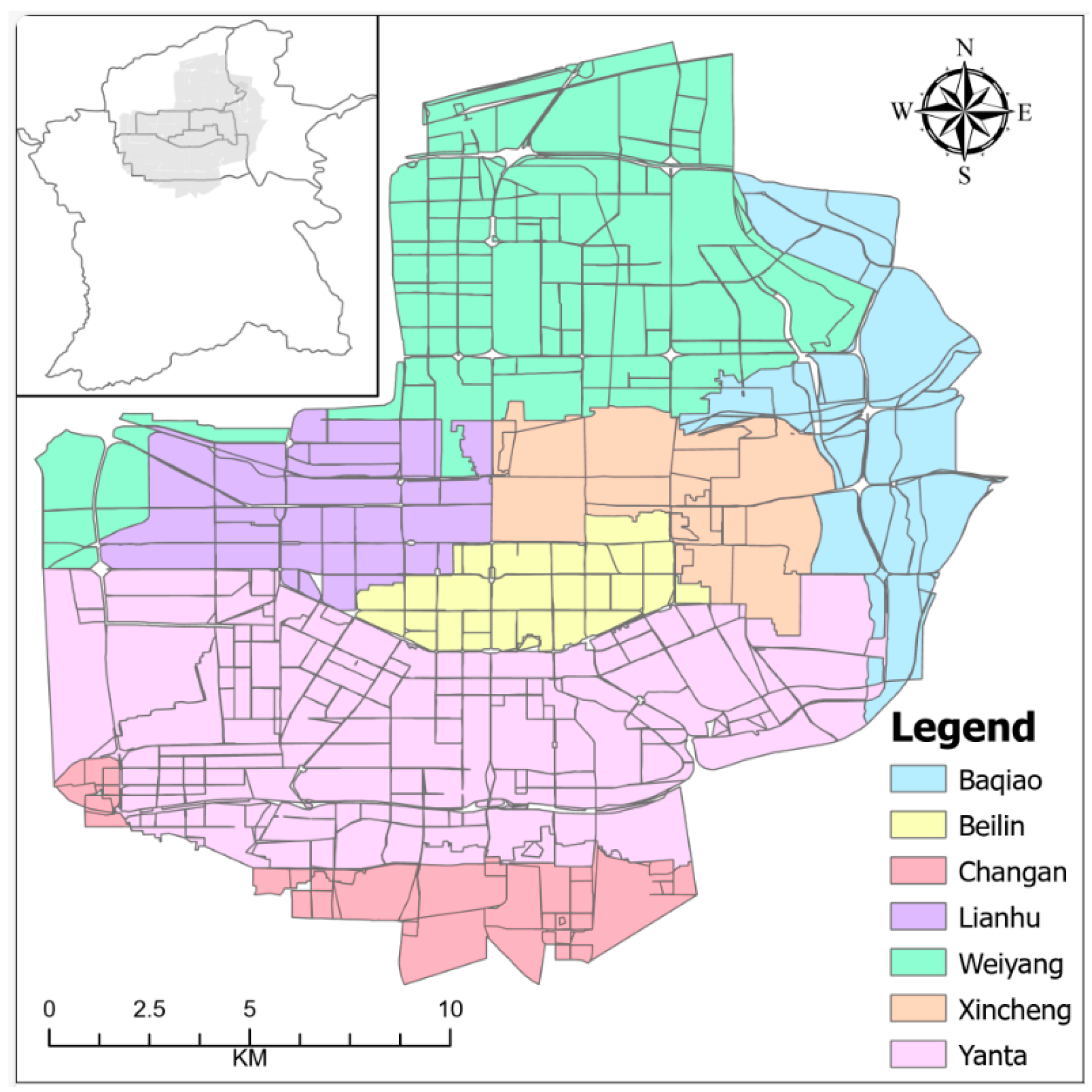
3.1. Study Area

Xi’an, with a total area of 10,108 square kilometers and a permanent population of 12.9959 million, is a central city in the northwest region of China. The number of vehicles in Xi’an increased from 180,000 in 1997 to 4.02 million by 2021 due to the rapid expansion of urban roads and a substantial influx of population. This study focuses on the area within Xi’an’s 3rd Ring Road, which is a prominent urban center characterized by dense population and commercial activities, as well as facing serious congestion issues. To thoroughly analyze the congestion in this area, we divided the study area into 680 separate plots based on the main road network and land properties. After a meticulous selection process to exclude smaller units, 520 effective plots were identified as the subjects of this study, as illustrated in Figure 1.

3.2. Data Introduction

In this study, land use data and mobile signaling data were used from the perspectives of traffic planning and congestion mitigation, offering new insights into individual travel trajectories and land distribution under different activities. The integration and analysis of these datasets primarily aimed to investigate the root causes of congestion from external factors of the transportation system. Specifically, mobile signaling data can identify travel trajectories, congested roads, travel OD (Origin-Destination) volumes, and residential population numbers, while POI (Point of Interest) can pinpoint the spatial distribution of different land uses. By analyzing these multi-source datasets, this research reveals potential causes of congestion, identifies the main external factors contributing to traffic congestion, and proposes targeted strategies to alleviate congestion in urban areas.

(1) The land use data primarily reflects the land development status within the study area, including POI and road network data. POI data, such as businesses, restaurants, financial institutions, etc., are sourced from the Gaode development platform. Additionally, road network data are obtained from OpenStreetMap.

(2) Mobile signaling travel data are provided by the “Smart Footprint” company, with the original data coming from China Unicom. To ensure data security, the platform sets the user ID as a prohibited field (not accessible by users), allowing only aggregated data to be exported for users. The data description is illustrated in

Table 1. Data description.

Item	Type	Explanation
Uid	String	The unique identifier of a user
time	Timestamp	The time when a user enters the road
route_id	Int	The unique identifier of road
rn_seq	Int	The sequential order of a road within the trip
is_start	Binary	Is it the starting point of the trip?
is_end	Binary	Whether it is the endpoint of the trip
trip_id	Int	The unique identifier for a user’s trip

, where the time extracts the time of entry into the road section, the route_id identifies the road section, the rn_seq recognizes the trajectory sequence, the is_start indicates whether it is the start of the trip, the is_end indicates whether it is the end of the trip, and the trip_id indicates the sequence number of the trip within a day for a user.

3.3. Built Environment Variables

In this paper, 12 variables were selected from land use, transportation-related, and socio-economic aspects. The land use variables included shopping center density, community services density, recreational density, catering density, financial institutions density, company enterprise density, educational services density, and land-use mix. The transportation-related variables included road density and transit station density, and the socio-economic variables included residential population density and working population density. To analyze these variables, we calculated the Mean and Standard Deviation (Std) for each, and further computed the Variance Inflation Factor (VIF). The results of VIF indicated that all variables had VIF values less than 5, suggesting the absence of multicollinearity issues. The descriptive statistics of the variables are shown in

Table 2. Descriptive statistics for variables.

Variables	Description	Mean	Std	VIF
Dependent variable
Congestion Contribution	The ratio of a plot’s congestion contribution to its area (persons/km2)	105.71	148.61	1.67
Independent variable: land use variables
Shopping Center Density	Ratio of the number of shopping centers to the area of the plot (units/km2)	195.02	261.98	2.98
Community Services Density	Ratio of number of amenity services to the area of the plot (units/km2)	100.50	97.83	2.88
Recreational density	Ratio of the number of recreational uses to the area of the plot (units/km2)	8.430	17.51	2.89
Catering Density	Ratio of the number of food and beverage establishments to the area of the plot (units/km2)	138.64	149.87	4.47
Financial Institutions Density	Ratio of the number of financial institutions to the area of the plot (units/km2)	11.96	20.76	2.16
Company Enterprise Density	Ratio of the number of corporate enterprises to the area of the plot (units/km2)	59.89	111.81	1.98
Educational Services Density	Ratio of the number of KES to the area of the plot (units/km2)	37.13	38.53	3.94
Land Use Mix	Entropy index of POI types within the plot	1.91	0.33	3.07
Independent variable: transportation-related variables
Road Density	Ratio of the length of the road network to the area of the plot (km/km2)	54.35	109.73	1.37
Transit Stations Density	Ratio of the number of bus stops and metro stations to the area of the plot (units/km2)	1.01	2.48	1.29
Independent variable: socio-economic variables
Residential Population Density	Ratio of the total population living in the plot (persons/km2)	13,600.53	11,342.62	4.21
Working Population Density	Ratio of the total number of the population working in the plot (persons/km2)	7343.87	7360.35	4.36

.

3.4. Research Methodology

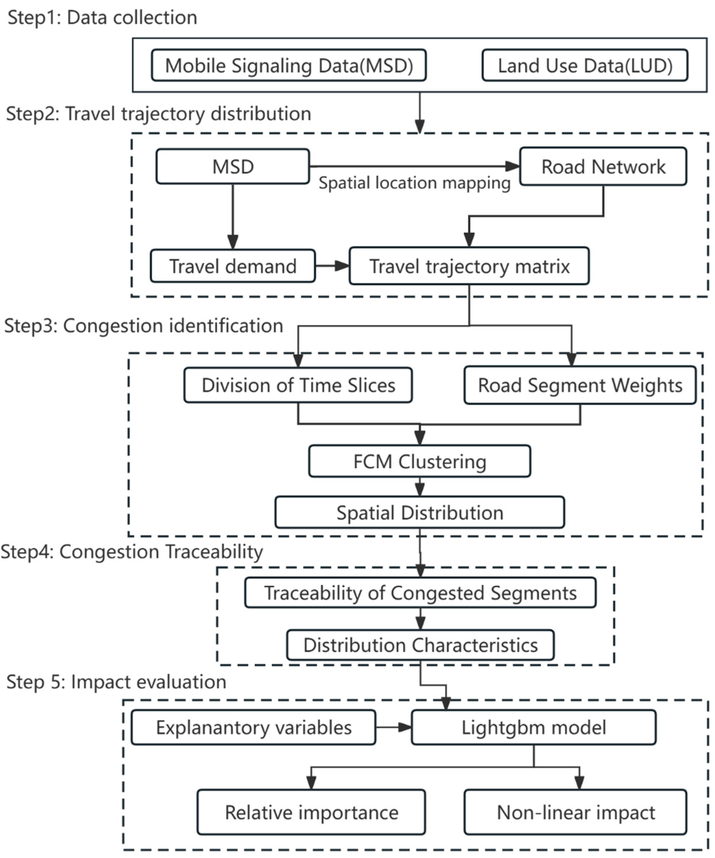
Figure 2 presents an analytical framework for investigating the distribution characteristics and influencing factors of congestion sources. Initially, mobile phone signaling data was mapped onto the road network to construct travel trajectory matrices. Subsequently, the data underwent time-slice processing to calculate the undirected weight values of roads in each time slice. The Fuzzy C-Means (FCM) clustering method was then applied to identify congested sections on expressways, main roads, and secondary roads. Following this, the origins of congested sections were traced to analyze the distribution characteristics of different source plots. Lastly, the LightGBM method was employed to study the impact of various factors on congestion contribution, revealing the non-linear relationships between these factors and congestion contribution.

3.4.1. Construction of Network Weights

In this study, we used the undirected weight value ${\mu }_{ij}$ to simplify the road network structure. For bidirectional traffic segments: if $K_{ij}<\frac{2}{3}$, it is assumed that the traffic distribution is balanced in both directions, and thus the segment’s undirected weight value is the average of the bidirectional weights. Conversely, if $K_{ij}\ge \frac{2}{3}$, it is assumed that the traffic distribution is significantly imbalanced, and in this case, the undirected weight value of the segment is taken as the weight value of the direction with heavier traffic load. For unidirectional traffic segments, the undirected weight value is the sole directional weight value. This is expressed in Equation (1).

$$u_{ij}=\left\{\begin{array}{l}{a}_{ij}{w}_{ij}+a_{ji}{w}_{ji},a_{ij}=1 or a_{ij}=1,a_{ji=0}\\ \frac{w_{ij}+w_{ji}}{2},a_{ij}=a_{ji}=1 and K_{ij}<\frac{2}{3}\\ \max \left\{w_{ij},w_{ji}\right\},a_{ij}=a_{ji}=1 and K_{ij}\ge \frac{2}{3}\end{array}\right.$$

(1)

In the formula, $w_{ij}(w_{j\mathrm{i}})$ represents the weight value of the edge from node i to node j (or from node j to node i). $a_{ij}$ indicates whether the network is connected from node i to node j. $K_{ij}$ denotes the directional distribution coefficient.

3.4.2. Fuzzy C-Means

The Fuzzy C-Means (FCM) algorithm is a clustering method for soft clustering, which establishes the affiliation of each sample data to all cluster centers by optimizing the objective, and classifies the sample data based on the size of the affiliation. Given the dataset $X=\{x_1,x_2,\cdots ,x_n\}$, it is assumed that the number of clusters is m, with $K={[k_1,k_2,\cdots ,k_m]}^T$ denoting the cluster center. $A={[u_{ij}]}_{n\times m}$ represents the fuzzy classification matrix, where $u_{ij}$ denotes the sample data $x_i$ to the clustering center $k_j$. The essence of the FCM algorithm is an iterative process that converges the objective function by continuously updating the cluster centers $K$ and the membership degree matrix $A$. The objective function is shown in Equation (2).

$$J(A,K)={\displaystyle {\sum }_{i=1}^n{\displaystyle {\sum }_{j=1}^m{u}_{ij}^t}}{‖x_i-k_j‖}^2 , 1.0\le m\le \infty$$

(2)

In this equation, $t$ represents the weighted exponent, which is commonly set to $t=2$. The algorithm steps are as follows:

(1) Determine the number of cluster centers m, set the iteration count $l=0$, and initialize the classification matrix $A={[u_{ij}]}_{n\times m}$.

(2) Calculate the affiliation matrix $A$ (Equation (3)).

$${\mu }_{ij}=\frac{1}{{\displaystyle {\sum }_{C=1}^{\mathrm{m}}{(\frac{‖x_i-k_j‖}{‖x_i-k_C‖})}^{\frac{2}{t-1}}}}$$

(3)

(3) Update the cluster centers $k_j$. (Equation (4)).

$$k_j=\frac{{\displaystyle {\sum }_{i=1}^n{\mu }_{ij}^t\cdot x_i}}{{\displaystyle {\sum }_{i=1}^n{\mu }_{ij}^t}}$$

(4)

Choose an appropriate norm $\epsilon >0$. If the condition $‖A^{l+1}-A^l‖<\epsilon$ is satisfied, terminate the operation; otherwise, let $l=l+1$ and repeat steps (3) and (4) until the condition is satisfied.

The classification coefficient is commonly used to evaluate the effectiveness of clustering algorithms. For a given number of clustering centers m and a classification matrix $A$, the classification coefficient is defined by Equation (5).

$$F=\frac{1}{n}{\displaystyle \sum _{i=1}^n{\displaystyle \sum _{j=1}^m{u}_{ij}^2}}$$

(5)

The classification coefficient is a standard indicating the fuzziness of clustering results; the closer $F$ is to 1, the better the clustering effect.

3.4.3. Traceability of Congested Segments

In this study, we define P as the set of all plots within the research area. For any two plots a and b, we are concerned with the set of travel ODs (Origin-Destination) from plot a to plot b, denoted as (a, b). Additionally, $crowd$ represents the set of congested roads in the area. Based on this, $q_{ab}$ is defined as the number of travelers from plot $a$ to plot $b$, and $r_{ab}$ represents the set of paths taken by these travelers. Specifically, ${r^l}_{ab}({r^l}_{ab}\in r_{ab},l\in crowd)$ denotes the set of travel trajectories passing through a specific congested segment $l$. The number of travelers passing through congested segment $l$ from plot a to plot b is $Q_{abl}$. The contribution of plot a to congested segment $l$ during the selected time period is expressed in Equation (6).

$$C{O}_l(a)={\displaystyle \sum _{b\in P}{\displaystyle \sum _{r_{ab}^l}{Q}_{abl}}}$$

(6)

3.4.4. LightGBM Model

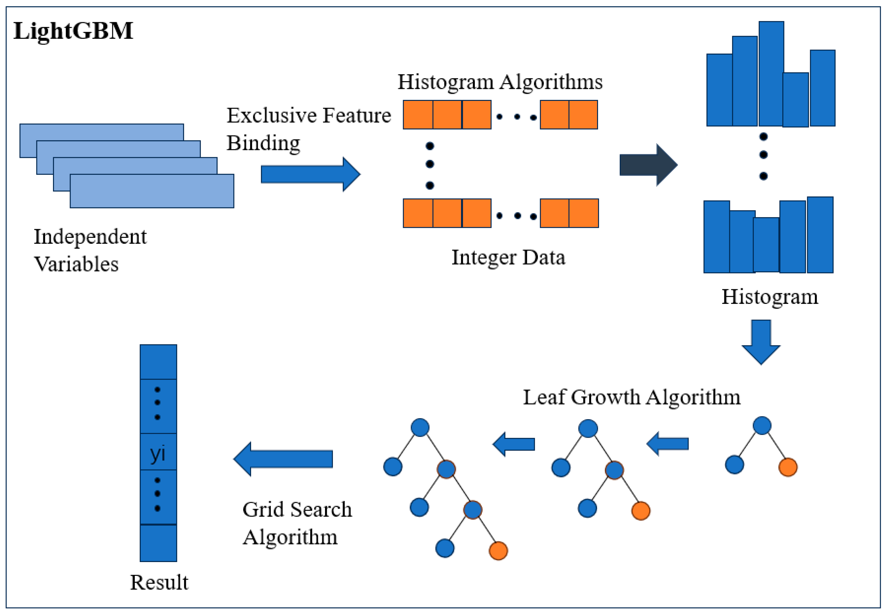
LightGBM is an advanced iterative decision tree algorithm, exhibiting significant advantages in efficiency and space usage compared to traditional models like GBDT. This is primarily attributed to its integration of two innovative technologies: Gradient-based One-Side Sampling (GOSS) and Exclusive Feature Bundling (EFB). GOSS significantly reduces computational load by retaining samples with larger gradient values while randomly sampling those with smaller gradients, thus enhancing the model’s efficiency. On the other hand, EFB, leveraging the sparsity of high-dimensional data, combines exclusive features, ensuring both the integrity of information and a reduction in feature dimensions. Additionally, LightGBM employs a histogram-based strategy for node splitting in decision trees, effectively identifying and splitting features that offer the maximum information gain. It also utilizes a leaf-wise growth strategy with depth limitations, which not only ensures efficiency but also effectively prevents overfitting by choosing the leaf with the maximum splitting gain for splitting. The structure and main experimental procedure of the LightGBM model are elaborately illustrated in Figure 2. This algorithm excels in handling large-scale datasets, particularly suitable for machine learning tasks that demand high efficiency and accuracy. The structural details and primary experimental flow of the LightGBM model are depicted in Figure 3.

In this study, the dataset was randomly divided into a training dataset and a validation dataset at a ratio of 7:3, with the training dataset being utilized for model fitting. Subsequently, the Grid Search algorithm was employed to adjust several hyperparameters, including the lambda_l1, lambda_l2, min_data_in_leaf, num_leaves, and feature_fraction, to identify the optimal parameter combination. Thereafter, the predictive capability of the LightGBM model was assessed using the validation dataset. The model’s performance was evaluated through statistical metrics such as the coefficient of determination (R²), Root Mean Square Error (RMSE), and Mean Absolute Error (MAE). Finally, the model was interpreted through feature importance and partial dependence plots.

4. Results

4.1. Congestion Identification Results

The time of 20 July 2021 was chosen for analysis due to the significant traffic congestion caused by heavy rainfall on that day. The data of the three types of roads were clustered in Python using the FCM algorithm and the results are shown in

Table 3. Range of congestion thresholds.

Road Class	Smooth Traffic	Mild Congestion	Moderate Congestion	Severe Congestion
expressway	[1, 0.8515)	[0.8515, 0.6200)	[0.6200, 0.3376)	[0.3376, 0)
trunk road	[1, 0.8128)	[0.8128, 0.6077)	[0.6077, 0.3562)	[0.3562, 0)
secondary road	[1, 0.7755)	[0.7755, 0.5448)	[0.5448, 0.2964)	[0.2964, 0)

The value of 1 is considered of a free-flow state, with smaller values indicating increasing congestion.

. The congestion levels were classified into four categories: smooth traffic, mild congestion, moderate congestion, and severe congestion. The table reveals that the clustering centers for the three road types are not significantly different, but the threshold decreases as the road grade lowers.

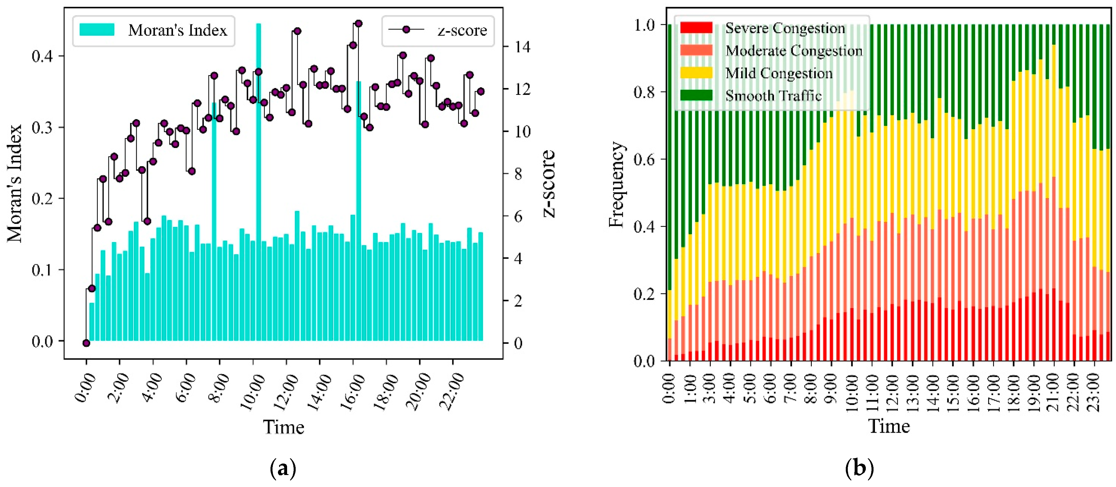
The spatial distribution and frequency characteristics of congestion status at different times were further analyzed, as shown in Figure 4. Figure 4a reveals the spatial autocorrelation numbers for each time node, with a time granularity of 20 min. The study utilized the Fuzzy C-Means (FCM) method to ascertain that the traffic congestion status within Xi’an’s third ring road is fundamentally correlated with space and exhibits a positive correlation throughout the day. Specifically, during the morning rush hour, the spatial distribution exhibits the highest degree of clustering and the highest level of congestion, with the peak Moran’s index observed at 10:00 a.m. This phenomenon suggests that targeted congestion management strategies during these peak hours could be highly effective, especially in clustered areas where congestion is most pronounced. As time progresses, the correlation between congestion intensity and spatial distribution remains stable, with certain clustering characteristics in the spatial distribution. Figure 4b illustrates the frequency of occurrence for each congestion level, using a 24-h daily granularity. From 0:00 to 6:00 a.m., the traffic network is at a low due to the rest period, with fewer residents traveling and the congestion level generally remaining unimpeded. Starting from 7:00 a.m., with the onset of the morning rush hour, the frequency of unimpeded road sections gradually decreases, and the level of congestion progressively increases, peaking around 10:00 a.m. Post noon, the congestion status undergoes slow changes until 18:00, when the congestion trend starts to intensify significantly, reaching its peak around 21:00. The sharp increase in congestion in the evening highlights the necessity for efficient public transit systems and real-time traffic management. The observed pattern of congestion intensification and subsequent easing further underscores the need for dynamic congestion management systems that can adapt to changing traffic conditions throughout the day.

4.2. Distribution of Congestion Sources

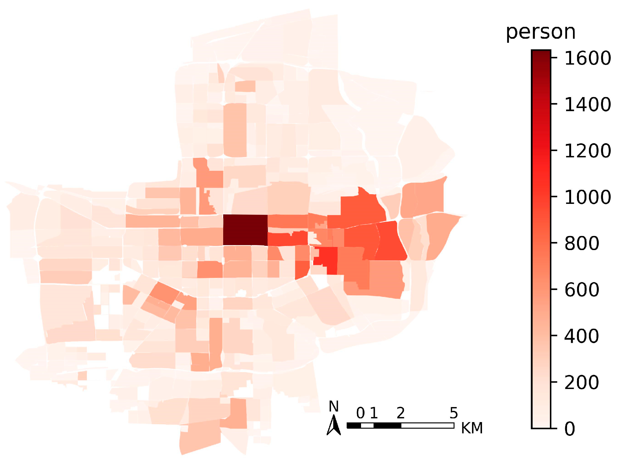
In response to the pronounced traffic congestion during the evening rush hour, this study selected this time period for a source analysis. After identifying the congested roads during the evening peak hours, the study further analyzed the origin distribution of travelers. As illustrated in Figure 5 (based on 20-min average travel flows), although the origins of travelers on congested roads are widespread, most areas contribute only limited travel flow. In contrast, there are fewer sources that significantly influence the main traffic flow, primarily concentrated within the city’s first ring and the residential areas on the right side between the first and second rings. The practical implications of these findings are profound, offering a nuanced understanding of congestion contributions. By identifying the primary sources of congestion, policymakers can tailor their approaches to address the specific needs and characteristics of the most impactful areas, thereby improving the efficiency of the transportation network. For example, promoting public transportation options or encouraging alternative modes of travel in these areas can help alleviate congestion throughout the entire region.

4.3. Impact Evaluation Results

4.3.1. Parameter Experiments

In this study, the suitable parameter combination for the LightGBM model is identified using the Grid Search algorithm (

Table 4. The tuning parameters of the LightGBM model.

Hyperparameter	Range	Value
lambda_l1	[0, 0.1, 0.2, 0.3, 0.4, 0.5, 0.6, 0.7, 0.8, 0.7]	0.1
lambda_l2	[0.5, 0.6, 0.7, 0.8, 0.9, 1]	0.6
min_data_in_leaf	[10, 20, 30, 40, 50, 60]	30
num_leaves	[10, 20, 30, 40, 50, 60, 70]	20
feature_fraction	[0.4, 0.5, 0.6, 0.7]	0.5

). This combination effectively prevents model overfitting and significantly enhances the model’s predictive accuracy by controlling parameters such as the lambda_l1, lambda_l2, min_data_in_leaf, num_leaves, and feature_fraction. Additionally, the robustness of the LightGBM model optimized through Grid Search is further evaluated using Five-fold Cross-validation. This involves calculating R², RMSE, and MAE for each test set, with results shown in

Table 5. Results of five-fold cross-validation.

Five-Fold Cross-Validation	RMSE	MAE	R2
0	149.48	97.08	0.71
1	162.99	114.61	0.56
2	137.83	115.02	0.69
3	153.26	121.15	0.55
4	124.69	91.57	0.58

. Among the five subsets, the R² values ranged from 0.55 to 0.71, RMSE values are between 124.69 and 162.99, and MAE values vary from 91.57 to 121.15. These results demonstrate that the LightGBM model exhibits good robustness.

4.3.2. Ranking of Independent Variable Importance

Table 6. Order of importance of independent variables.

Category	Variable	Rank	MRI (%)	Mean (%)
Land use variables	Shopping Center Density	7	7.55	7.29
	Community Services Density	10	6.04
	Recreational Density	9	7.13
	Catering Density	6	7.61
	Financial Institution Density	8	7.25
	Company Enterprise Density	5	8.46
	Educational Services Density	12	4.84
	Land Use Mix	4	9.43
Transportation-related variables	Road Density	2	12.27	9.16
	Transit Stations Density	11	6.04
Socio-economic variables	Residential Population Density	1	12.93	11.69
	Working Population Density	3	10.45

presents the mean relative importance (MRI) of different independent variables on the contribution to network-level congestion. The results indicate that socio-economic variables have the highest average importance, accounting for 11.69%, signifying their most significant impact on congestion contribution. This is primarily because areas with more developed economies typically have higher travel demands, leading to network-level congestion. In comparison, the importance of traffic-related characteristics is slightly lower, at 9.16%. Furthermore, the average importance of land-use characteristics is 7.29%, suggesting that land features also influence network-level congestion to a certain extent.

On the level of individual variables, residential population density is of the highest importance, with a significance of 12.93%, followed by road density at 12.27%. Working population density ranks third among all built-environment variables, with an importance of 10.45%. Additionally, land use mix, company enterprise density, catering density, and shopping center density also demonstrate significant predictive capabilities.

4.3.3. Non-Linear Relationships between Variables and Congestion Contributions

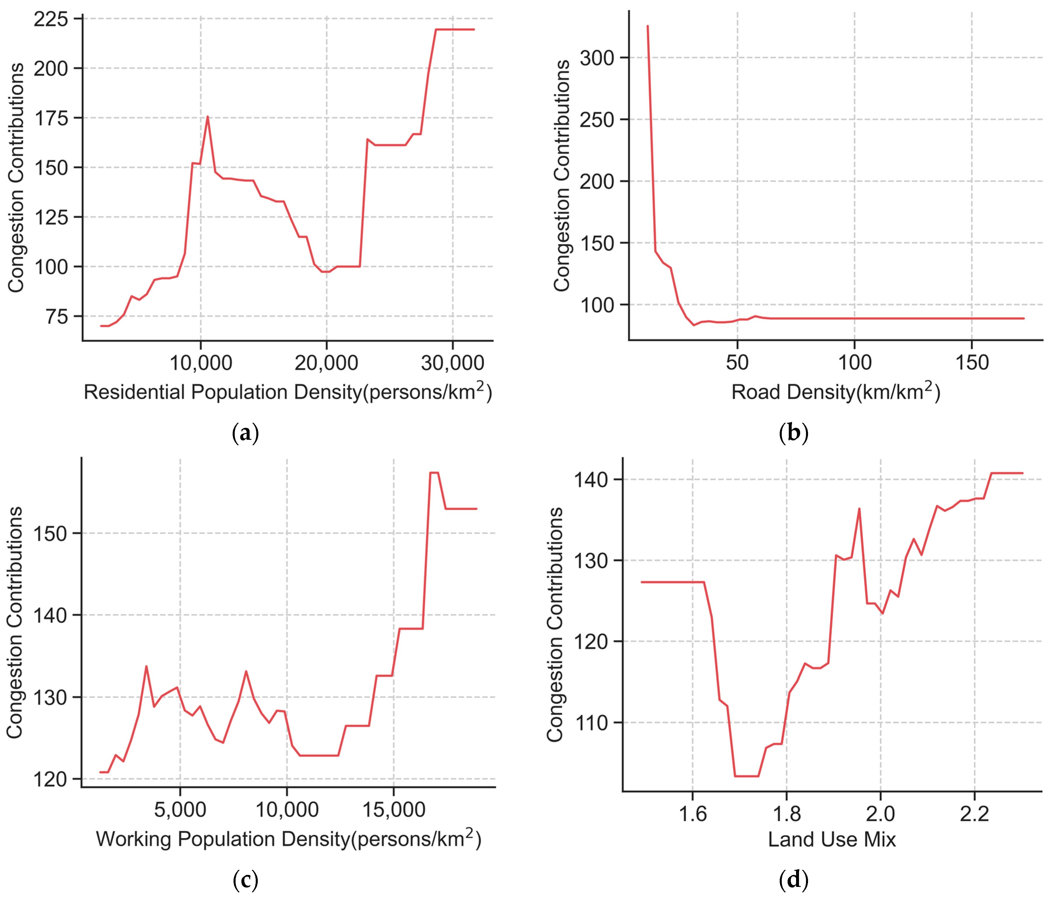
The four most important factors affecting the amount of congestion contribution were extracted and analyzed in a partial dependency diagram (PDP, Figure 6). These factors are residential population density, road network density, workforce population density, and land-use mix. The plots reveal a clear threshold effect of these four built-environment variables on congestion contribution.

Figure 6a illustrates the N-shaped correlation between residential population density and congestion contribution. The analysis reveals a significant increase in the impact of residential population density on congestion contribution as it escalates from 4000, peaking at 11,000. Beyond this peak, the trend inversely declines until reaching 20,000, indicating a complex interplay where additional population density does not linearly translate to increased congestion. It suggests that certain thresholds of population density may activate more efficient use of available transportation infrastructure, or a saturation point where the incremental impact on congestion diminishes. Subsequently, the trend witnesses a pronounced increase once more as the density escalates to 26,000. This resurgence underscores the overwhelming effect of very high residential population densities. Even with increased public transportation usage, the significant growth in travel demand leads to an increase in congestion contribution.

Figure 6b reveals the relationship between road density and congestion contribution, displaying a sharp downward trend. This decline peaks at a road density of 50, then stabilizes, indicating that higher road densities provide more route options, thus reducing congestion. This inverse correlation suggests that strategic increases in road infrastructure in densely trafficked areas can effectively alleviate congestion. However, the stabilization of this trend beyond a certain density highlights the diminishing returns of simply adding more roads, pointing towards the necessity for smarter traffic management and infrastructure development strategies that go beyond road expansion.

Figure 6c shows the relationship between working population density and congestion contribution, exhibiting a positive correlation with a distinct threshold effect. The congestion contribution decreases around a working population density of 8000 but significantly increases beyond 12,000, peaking at approximately 16,300. This pattern reflects the critical role of the working population’s movement patterns, especially during rush hours, in exacerbating congestion. It underscores the potential benefits of policies aimed at dispersing work start times or promoting remote work arrangements to ease peak congestion pressures. Moreover, this insight into the congestion contribution of the working population can guide targeted interventions in urban transport planning, such as the enhancement of public transit services or the development of new mobility solutions tailored to the needs of working individuals.

Figure 6d demonstrates the relationship between land use mix and congestion contribution, overall displaying a V-shaped pattern. Specifically, the congestion contribution sharply declines in a near-linear fashion within the land-use mix range of about 1.6–1.7. Beyond 1.73, the congestion contribution significantly increases, peaking around 1.9. However, the congestion contribution rises again beyond a land-use mix of two. Given the continuous increase thereafter, caution should be exercised with land-use mixes above 1.8.

5. Discussion and Conclusions

In summary, this study identified the congestion and traced its origins, exploring the explicability of different factors in network-level congestion contributions. Compared to previous research [25,26,27], our study discriminated congestion from a macro perspective and considered network structure, offering new insights into the dynamics of traffic congestion.

Our work shows that congestion clustering centers, which represent the degree of traffic congestion, are influenced by road levels, with congestion thresholds decreasing as road levels lower. Despite congestion being a ubiquitous issue across all road types, its severity becomes more pronounced on lower-level roads. Moreover, a stable positive correlation between congestion status and geographic location was observed, indicating significant spatial clustering. This suggests that congestion is not random but closely linked to specific geographic areas, emphasizing the importance of location-specific strategies in congestion mitigation for urban planners and traffic managers.

In addition, we traced the geographic origins of congestion, identifying the location where the travelers who participate in the network congestion primarily originate from. Interestingly, we found that a few spots are responsible for the majority of network congestion, primarily located in city centers and their surrounding areas. Therefore, optimizing traffic flow within these areas is essential for improving overall traffic efficiency. For example, promoting public transportation options in these areas or alternative routes to divert traffic from these congested hotspots could help alleviate congestion in the entire region [10,11].

Furthermore, we delved into the explicability of different factors contributing to network-level congestion. Unlike previous studies that focused on internal factors like traffic facilities and signal control [15,16], our study reveals the impact of external factors on congestion. The results indicate that residential population density is the most significant factor causing congestion. Additionally, road density, working population density, and land use mix also have considerable impacts on congestion. Notably, our study uncovered significant non-linear relationships between some built environment variables and congestion factors, notably the thresholds for residential population density and land use mix. This highlights the complex interplay between urban planning decisions and congestion outcomes, suggesting a more comprehensive approach to urban development strategies that consider how population dynamics, infrastructure capacity, and land use patterns collectively impact congestion. We recommend that efforts to mitigate congestion should not only aim to expand road capacity but also manage demand through housing planning, zoning regulations, and the promotion of mixed-use developments to reduce the necessity for long commutes.

In the end, this study has some limitations. First, congestion is considered not only in terms of the impact of the built environment variables but also requires further examination of specific aspects or influencing factors of congestion to explore the causes of congestion from a more comprehensive perspective. Second, this study highlights the significant impact of residential population density and working population density on congestion. Future research could delve deeper into how the travel patterns of different population groups (such as commuters, students, etc.) affect urban congestion. Finally, this study observes cyclical variations in congestion levels at different times of the day. Future research could further explore the spatiotemporal characteristics of congestion over longer periods or during special events (such as heavy rain or large-scale events) to provide a more detailed understanding of congestion dynamics.

References

- People’s Daily (PRC Newspaper). Many Countries Are Actively Exploring New Ideas to Combat Congestion (International Viewpoint). Available online: https://world.gmw.cn/2020-08/21/content_34106239.htm?from=search (accessed on 29 December 2023).
- Bao, Z.; Ng, S.T.; Yu, G.; Zhang, X.; Ou, Y. The effect of the built environment on spatial-temporal pattern of traffic congestion in a satellite city in emerging economies. Dev. Built Environ. 2023, 14, 100173. [Google Scholar] [CrossRef]
- SOHU. The Impact of Traffic Congestion on Us. Available online: https://www.sohu.com/a/227929997_99964784 (accessed on 5 February 2024).
- Chan, C.K.; Yao, X. Air pollution in mega cities in China. Atmos. Environ. 2008, 42, 1–42. [Google Scholar] [CrossRef]
- Ren, Y.; Shen, L.; Wei, X.; Wang, J.; Cheng, G. A guiding index framework for examining urban carrying capacity. Ecol. Indic. 2021, 133, 108347. [Google Scholar] [CrossRef]
- Li, Y.; Xiong, W.; Wang, X. Does polycentric and compact development alleviate urban traffic congestion? A case study of 98 Chinese cities. Cities 2019, 88, 100–111. [Google Scholar] [CrossRef]
- Yang, H.; Li, M.; Guo, B.; Zhang, F.; Wang, P. A vector field approach for identifying anomalous human mobility. IET Intell. Transp. Syst. 2023, 17, 649–666. [Google Scholar] [CrossRef]
- Zhang, D. Research on Urban Traffic Congestion Propagation Mechanism Analysis and Prediction Method Based on Multi-source GPS Data. Bachelor’s Thesis, Shenzhen University, Shenzhen, China, 2021. [Google Scholar]
- Wang, P.; Hunter, T.; Bayen, A.M.; Schechtner, K.; González, M.C. Understanding Road Usage Patterns in Urban Areas. Sci. Rep. 2012, 2, 1001. [Google Scholar] [CrossRef]
- Wang, P.; Wang, C.; Lai, J.; Huang, Z.; Ma, J.; Mao, Y. Traffic control approach based on multi-source data fusion. IET Intell. Transp. Syst. 2019, 13, 764–772. [Google Scholar] [CrossRef]
- Wang, J.; Wei, D.; He, K.; Gong, H.; Wang, P. Encapsulating Urban Traffic Rhythms into Road Networks. Sci. Rep. 2014, 4, 4141. [Google Scholar] [CrossRef] [PubMed]
- Li, M.; Yang, H.; Guo, B.; Dai, J.; Wang, P. Driver Source-Based Traffic Control Approach for Mitigating Congestion in Freeway Bottlenecks. J. Adv. Transp. 2022, 2022, 3536979. [Google Scholar] [CrossRef]
- Wang, C.; Xu, Z.; Du, R.; Li, H.; Wang, P. A vehicle routing model based on large-scale radio frequency identification data. J. Intell. Transp. Syst. 2020, 24, 142–155. [Google Scholar] [CrossRef]
- Wang, C.; Wang, P. Data, Methods, and Applications of Traffic Source Prediction. In Transportation Analytics in the Era of Big Data; Ukkusuri, S.V., Yang, C., Eds.; Springer International Publishing: Cham, Switzerland, 2019; pp. 105–120. [Google Scholar]
- Song, J.; Zhao, C.; Zhong, S.; Nielsen, T.A.S.; Prishchepov, A.V. Mapping spatio-temporal patterns and detecting the factors of traffic congestion with multi-source data fusion and mining techniques. Comput. Environ. Urban Syst. 2019, 77, 101364. [Google Scholar] [CrossRef]
- Yue, C.; Changle, L.; Wenwei, Y.; Hehe, Z.; Guoqiang, M. Root Cause Identification for Road Network Congestion Using the Gradient Boosting Decision Trees. In Proceedings of the GLOBECOM 2020—2020 IEEE Global Communications Conference, Taipei, Taiwan, 7–11 December 2020; p. 6. [Google Scholar]
- Vlahogianni, E.I.; Karlaftis, M.G.; Golias, J.C. Short-term traffic forecasting: Where we are and where we’re going. Transp. Res. Part C-Emerg. Technol. 2014, 43, 3–19. [Google Scholar] [CrossRef]
- Kamarianakis, Y.; Prastacos, P. Space–Time modeling of traffic flow. Comput. Geosci. 2005, 31, 133. [Google Scholar] [CrossRef]
- Liang, X.; Chen, S.; Li, D. Diagnosis and analysis of congested sections of urban road network based on WGN algorithm. Sci. Technol. Eng. 2021, 21, 11783–11789. [Google Scholar]
- Wang, Q.; Xie, Y.; Duan, H.; Li, J.; Zhao, D. A Study of Traffic Congestion in Xi’an Based on Real-Time Road Condition. J. Northwestern Univ. Nat. Sci. Ed. 2017, 47, 622–626. [Google Scholar] [CrossRef]
- Zhu, L.; Wen, X.; Zhang, J.; LIU, H.; Li, M. Urban Traffic Congestion Section Discrimination Based on Bus Floating Vehicle Data. J. Wuhan Univ. Technol. Transp. Sci. Eng. Ed. 2021, 45, 666–671. [Google Scholar]
- Jiang, Y. Traffic Congestion Discrimination and Prediction Based on Spatio-Temporal Correlation Analysis. Master’s Thesis, North Industrial University, Beijing, China, 2019. [Google Scholar]
- Zhang, J. Traffic Congestion Determination, Diversion and Simulation on Urban Roads. Doctoral Thesis, Southeast University, Nanjing, China, 2017. [Google Scholar]
- Zhao, L.; Xu, T.; Zhang, Z.S.; Hao, Y.J. Lane-Changing Recognition of Urban Expressway Exit Using Natural Driving Data. Appl. Sci. 2022, 12, 9762. [Google Scholar] [CrossRef]
- Yang, H. A Study on the Evolution of Frequent Urban Traffic Congestion Based on Taxi GPS Data. Doctoral Thesis, Harbin Institute of Technology, Harbin, China, 2019. [Google Scholar]
- Kong, X.; Xu, Z.; Shen, G.; Wang, J.; Yang, Q.; Zhang, B. Urban traffic congestion estimation and prediction based on floating car trajectory data. Future Gener. Comput. Syst. 2016, 61, 97–107. [Google Scholar] [CrossRef]
- Liu, Z.; Li, H.; Kang, H. Real-time Discriminative Algorithm Implementation for Lane Congestion at Urban Highway Intersections Based on YOLOv3. Electron. Prod. 2020, 2020, 40–41+37. [Google Scholar] [CrossRef]
- Zeng, J.; Xiong, Y.; Liu, F.; Ye, J.; Tang, J. Uncovering the spatiotemporal patterns of traffic congestion from large-scale trajectory data: A complex network approach. Phys. A Stat. Mech. Its Appl. 2022, 604, 127871. [Google Scholar] [CrossRef]
- Wang, X.; Wang, X.; Xin, X. Urban Residents’ Commuting, Land Use Layout and Traffic Congestion—An Empirical Study Based on Area Scale. Fudan J. Nat. Sci. Ed. 2018, 57, 199–204. [Google Scholar] [CrossRef]
- Zhang, T.; Sun, L.; Huang, Y.; Zhou, L.; Zeng, W. Study on the Relationship between Traffic Congestion and Land Use Based on Real-time Network Data--Taking Tianjin Binhai New Area as an Example. Transp. Stud. 2017, 3, 1–8. [Google Scholar] [CrossRef]
- Wang, M.; Debbage, N. Urban morphology and traffic congestion: Longitudinal evidence from US cities. Comput. Environ. Urban Syst. 2021, 89, 101676. [Google Scholar] [CrossRef]
- Sun, C.; Lu, J. The Relative Roles of Socioeconomic Factors and Governance Policies in Urban Traffic Congestion: A Global Perspective. Land 2022, 11, 1616. [Google Scholar] [CrossRef]
- Bao, Z.; Ou, Y.; Chen, S.; Wang, T. Land Use Impacts on Traffic Congestion Patterns: A Tale of a Northwestern Chinese City. Land 2022, 11, 2295. [Google Scholar] [CrossRef]
- Rothman, L.; Buliung, R.; Howard, A.; Macarthur, C.; Macpherson, A. The school environment and student car drop-off at elementary schools. Travel Behav. Soc. 2017, 9, 57. [Google Scholar] [CrossRef]
- Zhang, T.; Sun, L.; Yao, L.; Rong, J. Impact Analysis of Land Use on Traffic Congestion Using Real-Time Traffic and POI. J. Adv. Transp. 2017, 2017, 7164790. [Google Scholar] [CrossRef]
- Wang, D.; Chen, H.; Li, C.; Liu, E. Exploring the Relationship between Land Use and Congestion Source in Xi’an: A Multisource Data Analysis Approach. Sustainability 2023, 15, 9328. [Google Scholar] [CrossRef]
- Liu, J.; Xiao, L. Non-linear relationships between built environment and commuting duration of migrants and locals. J. Transp. Geogr. 2023, 106, 103517. [Google Scholar] [CrossRef]
- Li, L.; Zhong, L.; Ran, B.; Du, B. Analysis of the relationship between metro ridership and built environment: A machine learning method considering combinational features. Tunn. Undergr. Space Technol. 2024, 144, 105564. [Google Scholar] [CrossRef]