Research on the Spatial Disparities and Convergence of Guangdong’s Urban Economy Based on Industrial Agglomeration and Industrial Proximity

Abstract

Understanding the spatial differences and evolutionary characteristics of urban economy and exploring the impact of industrial agglomeration and industrial proximity on urban economic convergence are the bases for scientifically formulating policies for coordinated regional economic development. This study used QGIS 3.10.10 software and the Theil index to analyze the spatial distribution characteristics and regional disparities of urban economy. Then, a spatial econometric model was constructed to analyze the convergence and influencing factors of Guangdong’s urban economy. The results indicate that from 2006 to 2020, Guangdong’s urban economy grew rapidly and the degree of economic agglomeration gradually weakened, but its economic pattern always maintained the “Core-Edge” structural feature. The interval disparities between the Pearl River Delta Urban Agglomeration (PRD) and the edge area have always been greater than the intra-regional disparities, so they are main source of disparities in Guangdong. In Guangdong’s urban economy, σ-convergence and β-convergence coexist. The conditional β-convergence rate is 0.96~1.53%, and the half-life cycle is 45.4~72.36 years. Compared to the PRD, the economic disparities in the edge area are smaller but the convergence speed is faster and the half-life cycle is shorter. Both industrial agglomeration and industrial proximity have a significant impact on the economic convergence of Guangdong’s cities. Among them, industrial agglomeration has a positive impact, while industrial proximity has a negative impact. There is spatial heterogeneity in the impact of industries on economic development. Industrial agglomeration has a positive impact on the overall economic development of Guangdong, but it is not significant within the regions. Industrial proximity has significant negative externalities in the PRD region, and its impact is not significant in the edge area.

1. Introduction

Unbalanced regional economic development is one of the prominent problems that have long existed in China’s economic development [1]. Therefore, as a geographical phenomenon of unbalanced development, regional growth disparity has always been the focus of academic and political circles [2]. At present, China’s economy is in a transition period from high-speed growth to high-quality development. The 19th National Congress of the Communist Party of China proposed firmly implementing the strategy of regional coordinated development and establishing a more effective new mechanism for regional coordinated development. Objectively describing the current situation of regional economic disparities and convergence is the basic premise for formulating positive policies to enhance regional development coordination.

The economic convergence hypothesis provides a description for the less developed regions to narrow the gap with the developed regions [3]. If convergence is established, then the gap between the rich and the poor will be narrowed. Scholars mostly acknowledge that China’s global economy has gone through a process of “convergence divergence convergence” [4,5]. There are club convergence characteristics in the regional differences divided by the east, middle, west, or north and south [4,5]. The difference in economic development is ultimately caused by the disparity in the allocation and utilization of production factors between regions. But the flow and allocation of production factors not only depend on the price adjustment mechanism of the factor market but also on the industrial organization mode and characteristics within a specific industry. With the rapid growth of the Chinese economy, the urban industrial structure has also undergone significant adjustments, and regional layout is undergoing drastic changes. In the process of changing the industrial layout, due to the increasing returns to scale and positive external economic benefits, some regions have become the “centers” of industrial agglomeration due to their superior conditions. Therefore, the formation and evolution mechanism of industrial agglomeration will definitely have an impact on economic convergence and may even become a decisive factor in the change of regional disparities. There are two different views on the understanding of agglomeration economies in existing research. Some scholars believe that the current urban scale of China is still insufficient, and there is still much room for improvement in the level of agglomeration [4,6,7]. Agglomeration externalities have significant spatial spillover effects, which help to narrow regional economic disparities [8]. Another scholar believes that negative effects of agglomeration on the economy have emerged, the scale of megacities should be controlled, and the investment in small and medium-sized cities should be increased [9]. With the continuous subdivision of industries, scholars are not only concerned about the agglomeration characteristics of individual industries but also the co-location of industries [10]. Forming a reasonable industrial spatial division of labor pattern is also the key to coordinated development among cities. For a long time, scholars at home and abroad have been actively exploring how to promote the improvement in overall economic efficiency by guiding the adjustment of industrial structure. However, there is still controversy over whether cities should adopt industrial division policies or homogenization positioning strategies [11]. One viewpoint holds that the convergence of industrial structures within a region is a manifestation of vicious competition among industries within the region, and it is viewed negatively [12,13]. There is also a view that the convergence of regional industrial structures also has a “desirable” convergence [14]. The index of industrial structure similarity between regions reflects the level of industrial integration in the region [15,16]. The economic growth is not isolated in geographical space, and there is a flow of factors and spatial interaction between regions [17]. The increasing industrial connections between cities have made spatial spillover an important driving force for narrowing regional economic disparities [18,19,20]. Therefore, it is necessary to consider spatial spillover effects in economic convergence research.

Previous studies have typically used industrial agglomeration or industrial proximity as the explanatory variable, examining the impact of transportation, population, and natural resources on industrial agglomeration or inter-urban industrial structure similarity. There are few studies on the role of industrial agglomeration and industrial proximity in regional economic convergence. In this context, the main objective of this study is to reveal the impact of industrial agglomeration and convergence of industrial structure on economic convergence. In view of this, this study uses panel data from 21 cities in Guangdong from 2006 to 2020. First, various indexes are used to measure the spatial distribution characteristics and regional differences of urban economies. Secondly, a spatial econometric model is constructed to test the role of industrial agglomeration and convergence of industrial structure on regional economic convergence. The marginal contributions are as follows: (1) using the index method combined with spatial econometric models to reveal the economic differences and convergence of Guangdong’s cities; (2) revealing the mechanism of industrial agglomeration and convergence of industrial structure on regional economic convergence.

2. Theoretical Mechanism and Research Hypothesis

2.1. Industrial Agglomeration and Regional Economic Convergence

Industrial agglomeration is a form of regional industrial organization, and localized growth induced by industrial agglomeration in spatial economics has attracted widespread attention. Industrial agglomeration plays an important role in economic growth [4]. The scale effect brought by industrial agglomeration can reduce production costs and achieve increasing economic returns. The agglomeration region thus obtains positive externalities and develops faster economically. At this point, the agglomeration region will produce a “centripetal force” that attracts further agglomeration of factors and further expands regional differences. When the agglomeration exceeds a certain level, the exclusiveness of the market begins to emerge, and fierce market competition will cause certain crowding-out effects for enterprises. The “crowding-out effect” leads to industrial migration, which produces a “centrifugal force”. In the process of industrial migration, it is accompanied by the flow and diffusion of factors such as capital, technology, and human capital, which has a spillover effect on the surrounding region and is conducive to narrowing the gap in regional economic development. In view of this, we propose the following hypothesis:

H1. 

Industrial agglomeration can have a significant impact on regional economic convergence. When the “centripetal force” is stronger than the “centrifugal force”, industrial agglomeration will have a negative impact on regional economic convergence (H1a). When the “centrifugal force” is stronger than the “centripetal force”, industrial agglomeration will have a positive impact on regional economic convergence (H1b).

In addition, the gradient differences in the relative abundance of factors such as capital, technology, and human resources are the basis for the transfer, undertaking, and collaboration of industries in various regions. Therefore, we propose the hypothesis that:

H2. 

The promotion effect of industrial agglomeration on economic convergence is stronger in regions with large economic development differences.

2.2. The Convergence of Industrial Structure and Regional Economic Convergence

Industrial proximity refers to the phenomenon where the structural characteristics of industries, such as types and scale ratios, are similar among cities in a region [21]. Different cities within a region, excluding their special endowment resources, often have similar factor endowment structures. Similar endowment structures lead to similar comparative advantages, which in turn lead to the development of similar industries in various regions, resulting in industrial convergence. In this case, regional integration development will inevitably lead to industrial convergence [21]. Through imitation learning, industrial convergence can not only strengthen the positive externalities of technology but also bring late-mover advantages to less developed regions [22,23]. Therefore, it can bring positive spatial spillover effects [21]. There are also views that industrial convergence brought about by redundant construction and vicious competition will hinder economic development [24,25]. In view of this, we propose the hypothesis that:

H3. 

Industrial proximity can have a significant impact on regional economic growth. Industrial proximity brings positive externalities and promotes regional economic convergence (H3a). When industrial proximity leads to vicious competition, it will have a negative effect on regional economic convergence (H3b).

3. Overview of the Study Area and Materials

Guangdong is located in the south of China’s Nanling Mountains on the coast of the South China Sea. It is one of the earliest provinces to have undergone reform and opening up and one of the most economically dynamic provinces in China. Since 1989, Guangdong’s economic aggregate has ranked first in China—more than 30 years. The Pearl River Delta Urban Agglomeration (PRD) in Guangdong Province is one of the most influential urban agglomerations in China and plays an important leading role in Guangdong’s economic development. According to statistics, about 80% of the contribution of Guangdong’s Gross Domestic Product (GDP) comes from the PRD. In 2020, the GDP of the PRD was as high as CNY 8.94 trillion and the per-capita GDP was CNY 114,429, which are 4.22 times and 2.59 times those of the edge area. In addition, the PRD region is also one of the most important industrial agglomeration areas in China. The “core-edge” agglomeration economic pattern in the PRD and its surrounding areas is typical and representative. Therefore, we chose Guangdong as the research area to conduct research on industrial and economic convergence.

This study used the socio-economic data of 21 prefecture-level cities in Guangdong Province from 2006 to 2020. Among them, the data of GDP, resident population, area, government budget expenditure, fixed asset investment, foreign direct investment (FDI), research and development (R&D) expenditure, R&D personnel, number of industrial enterprises and added value of industrial sub-industries of each city were from the Guangdong Statistical Yearbook from 2007 to 2021 (http://stats.gd.gov.cn/gdtjnj/, accessed on 3 May 2023). The vector data of Guangdong city administrative divisions in 2019 come from the National Geographic Information Center (https://www.webmap.cn/main.do?method=index, accessed on 20 March 2021).The shortest driving time between cities in Guangdong is from the search results of Baidu Map (https://map.baidu.com/, accessed on 21 June 2021).

4. Methods

4.1. Regional Difference Analysis

The Theil coefficient can measure the gap of regional economic level. The higher the value is, the greater the regional economic difference is; otherwise, the smaller the economic difference is [26]. The formula is expressed as follows:

$$TL=\frac{1}{n}{{\displaystyle \sum }}_{i=1}^n\frac{y_i}{\mu }ln\frac{y_i}{\mu },$$

(1)

where $TL$ is the overall Theil index, n is the number of cities, $\mu$ is the average per-capita GDP of the cities, and $y_i$ refers to the per-capita GDP of city i.

The Theil coefficient can be further decomposed into interval disparities (T_b) and intra-regional disparities (T_w), enabling a more accurate identification of the sources of regional disparities [27]. The formula is expressed as follows:

$$\begin{array}{l}TL=T_{\mathrm{b}}+T_{\mathrm{w}}\\ T_{\mathrm{b}}={\displaystyle \sum _{k=1}^n\frac{n_k}{n}}\times \frac{n_k}{\mu }\times \ln \frac{n_k}{\mu }\\ T_{\mathrm{w}}={\displaystyle \sum _{k=1}^n\frac{n_k}{n}}\times \frac{n_k}{\mu }(\frac{1}{n}{\displaystyle \sum _{i\in gk}^n\frac{y_i}{y_k}}\ln \frac{y_i}{y_k})={\displaystyle \sum _{k=1}^n\frac{n_k}{n}}\times \frac{y_k}{\mu }\times T(y_k)\end{array},$$

(2)

where $y_k$ and $n_k$ refer to the average and quantity of per-capita GDP of the $k$-th group of cities, respectively. In this article, cities in Guangdong Province were divided into two groups: the PRD and the edge area. Among them, the PRD includes Guangzhou, Shenzhen, Dongguan, Huizhou, Foshan, Jiangmen, Zhongshan, Zhuhai, and Zhaoqing; the edge area includes Shantou, Shaoguan, Heyuan, Meizhou, Shanwei, Yangjiang, Zhanjiang, Maoming, Qingyuan, Chaozhou, Jieyang, and Yunfu.

4.2. Industry Analysis

4.2.1. Industry Agglomeration

The geographic agglomeration degree is used to characterize industry agglomeration. It is often used to reflect the degree of imbalance in the spatial distribution of regional economic factors [28]. The formula is expressed as follows:

$$R_{{}_{\mathrm{it}}}=\frac{X_{it}}{Y_{it}},$$

(3)

where $R_{it}$ denotes the geographical concentration of economic factors in unit $i$ at time $t$; $X_{it}$ represents the proportion of GDP in the unit $i$ at time $t$; and $Y_{it}$ represents the proportion of the total area of the region in the unit $i$ at time $t$.

4.2.2. Industrial Proximity

Industrial proximity ($IP$) is characterized by the industrial structure similarity coefficient. In 1979, the International Industrial Research Center of the United Nations Industrial Development Organization (UNIDO) proposed a structural similarity coefficient, which was used to measure the industrial structure similarity of countries to measure the degree of industrial proximity [29]. The formula is expressed as follows:

$$\begin{array}{l}I{P}_{ij}^{}=\{\begin{array}{c}\frac{{\displaystyle {\sum }_{k=1}^n(X_{ik}{X}_{jk})}}{\sqrt{{\displaystyle {\sum }_{k=1}^n{X}_{in}^2{\displaystyle {\sum }_{k=1}^n{X}_{jk}^2}}}}\begin{array}{cc}& \end{array}(i\ne j)\\ \begin{array}{l}\\ 0\begin{array}{cc}& \begin{array}{cc}\begin{array}{cc}\begin{array}{cc}& \end{array}& \end{array}& \end{array}\end{array}(i=j)\end{array}\end{array}\\ I{P}_i={\displaystyle \sum _{j=1}^m{S}_{ij}}\begin{array}{cc}& \end{array}(i\ne j)\end{array},$$

(4)

where $I{P}_{ij}$ is the industrial proximity coefficient of $i$ city and $j$ city. $X_{ik}$ and $X_{jk}$ represent the proportion of industrial added value of $k$ industry to the industrial added value of city $i$ and city $j$, respectively. $X_{ik}$ represents the proportion of $k$ industry added value in industrial added value in city $i$. $X_{jk}$ represents the proportion of $k$ industry added value in industrial added value in city $j$. $I{P}_i$ represents the industrial proximity between city $i$ and other cities within the study area. $m$ represents the number of cities; $m$ = 21. $n$ is the classification number of industrial industries. From 2006 to 2010, $n$ = 39; from 2011 to 2020, $n$ = 41.

4.3. Spatial Autocorrelation

The existence of significant spatial agglomeration is a prerequisite for empirical research using spatial econometric models. The spatial autocorrelation index is a common tool for measuring the spatial correlation of values. The global Moran’s I index is calculated as follows:

$$\begin{array}{l}I=\frac{{\displaystyle \sum _{i=1}^n{\displaystyle \sum _{j=1}^n{W}_{ij}(X_i-\overline{X})}(X_j-\overline{X})}}{S^2{\displaystyle \sum _{i=1}^n{\displaystyle \sum _{j=1}^n{W}_{ij}}}}, \mathrm{and}\\ S^2=\frac{1}{n}{\displaystyle \sum _{i=1}^n{(X_i-\overline{X})}^2}\end{array}$$

(5)

where the range of I is [−1, 1]; $X_i$ and $X_j$ are the attribute values of regions i and j; $\overline{X}$ is the average of the attribute values; n is the number of units studied; $W_{ij}$ is the spatial weight; and $S$² is the variance of the attribute values.

4.4. Economic Convergence Model

4.4.1. σ-Convergence

The σ-convergence represents the process of regional economic disparities narrowing over time [30]. Referring to the practice of predecessors [31], this paper used the time series change trend in the standard deviation of the logarithm of per-capita GDP to judge whether there is convergence.

$${\sigma }_t=\sqrt{\frac{1}{n}{{\displaystyle \sum }}_{i=1}^n{(ln{D}_{it}-\frac{1}{n}{{\displaystyle \sum }}_{i=1}^{n}ln{D}_{it})}^2},$$

(6)

where i and $t$ are city and year, respectively. $lnD$ represents the logarithm of per-capita GDP. ${\sigma }_t$ is the $t$-year convergence coefficient $\sigma$ value. If the ${\sigma }_t$ value shows a trend of convergence year by year, there is $\sigma$-convergence.

4.4.2. β-Convergence

• β-convergence and conditional β-convergence

The β-convergence judges whether there is convergence by observing the relationship between the urban economic growth rate and base period level [32]. If there is a significant negative correlation between the economic growth rate and the base period level, it means that the economic growth rate of underdeveloped areas is higher than that of developed areas, and the economy of the study area has β-convergence. The β-convergence can be divided into absolute β-convergence and conditional β-convergence [32,33].

The conditional β-convergence means that the region will be in a state of convergence when controlling other influencing factors, while the absolute β-convergence indicates that the region will also be in a state of convergence without controlling these factors [34]. The absolute β-convergence formula is expressed as follows:

$$\frac{1}{T}\ln (\frac{D_{i,t+T}}{D_{i,t}})=\alpha +\beta \ln D_{i,t}+{\epsilon }_{i,t},$$

(7)

The control variables affecting economic development are added to Formula (7) to construct a conditional β-convergence model. The formula is expressed as follows:

$$\frac{1}{T}\ln (\frac{D_{i,t+T}}{D_{i,t}})=\alpha +\beta \ln D_{i,t}+\theta X_{i,t}+\theta Z_{i,t}+{\epsilon }_{i,t},$$

(8)

where $D_{i,t}$ represents the per-capita GDP of city $i$ in period $t$, and $D_{i,t+T}$ is the per-capita GDP at the end of the period. It represents the growth rate of per-capita GDP of city $i$ in period $T$, and $T=1$ in the regression; that is, the annual growth rate of per-capita GDP is a constant term and an error term. If it is significantly less than 0, it indicates that the urban economy has convergence. $\theta$ is the regression coefficient of the variables. $X$ and $Z$ are the core variables and control variables, respectively (

Table 1. Main variables.

Type	Name	Unit	Description
Dependent variable ($D$)	Per-capital GDP	CNY	GDP/year-end permanent population
Core variables ($X$)	Industry agglomeration (R)	--	Calculated according to Formula (3)
	Industrial proximity (IP)	--	Calculated according to Formula (4)
Control variables ($Z$)	Investment (Inves)	CNY/person	Fixed asset investment/year-end permanent population
	Foreign direct investment (FDI)	%	Actual use of foreign direct investment/GDP
	Research and development (R&D)	CNY/person	R&D spending/year-end permanent population
	Government fiscal expenditure (fiscal)	CNY/person	Local general public budget expenditure/year-end permanent population

). The core variables include industrial agglomeration ($R$) and industrial proximity ($IP$). They have significant impacts on economic development, but their mechanisms of action are not yet clear. The control variables include investment (Inves), foreign direct investment (FDI), research and development (R&D) and government fiscal expenditure (fiscal). Investment and FDI are important influencing factors for regional economic growth [35,36]. As the foundation and key pillar of national governance, fiscal expenditure plays a positive role in improving economic efficiency and balancing regional development [37]. R&D can significantly promote industrial structure upgrading and is also an important driving force for economic growth [38]. $\epsilon$ is a random error term. To avoid heteroscedasticity, both the dependent variable and the independent variable are taken as logarithms.

2.

Conditional space β-convergence

In the process of regional economic convergence, spatial factors play an important role [39,40]. In order to avoid the bias of the estimation results, it is necessary to introduce spatial factors on the basis of the β-convergence model. The spatial autoregression model (SAR), spatial error model (SEM) and spatial Durbin model (SDM) are three commonly used spatial econometric models. The SAR model assumes that the explained variables affect regional economic growth through spatial interaction. The SEM represents the influence of error term transmission on economic growth. The SDM model considers both the spatial interaction of explanatory variables and the conduction of the error term [41].

SAR is added into the β-convergence framework, and it can be expressed as follows:

$$\frac{1}{T}\ln (\frac{D_{i,t+T}}{D_{i,t}})=\alpha +\beta \ln D_{i,t}+\rho W\ln (\frac{D_{i,t+T}}{D_{i,t}})+\theta \ln X_{i,t}+\theta \ln Z_{i,t}+{\epsilon }_{i,t},$$

(9)

SEM is added into the β-convergence framework, and it can be expressed as follows:

$$\begin{array}{l}\frac{1}{T}\ln (\frac{D_{i,t+T}}{D_{i,t}})=\alpha +\beta \ln D_{i,t}+\theta \ln X_{i,t}+\theta \ln Z_{i,t}+{\epsilon }_{i,t}\\ {\epsilon }_{i,t}=\lambda W{\epsilon }_{i,t}+{\mu }_{i,t}\end{array},$$

(10)

SDM is added into the β-convergence framework, and it can be expressed as follows:

$$\frac{1}{T}\ln (\frac{D_{i,t+T}}{D_{i,t}})=\alpha +\beta \ln D_{i,t}+\theta \ln X_{i,t}+\theta \ln Z_{i,t}+\rho W\ln (\frac{D_{i,t+T}}{D_{i,t}})+\delta W\ln D_{i,t}+\theta W\ln X_{i,t}+\theta W\ln Z_{i,t}+{\epsilon }_{i,t},$$

(11)

where $D_{i,t}$ represents the per-capita GDP of city $i$ in period $t$; $\alpha$ is a constant term. $\theta$ is the regression coefficient of the variables. $X$ and $Z$ are the core variables and control variables, respectively (Table 1). $\beta$ is the regression coefficient of the model. If $\beta$ < 0, it shows that the per-capita GDP of Guangdong’s cities has convergence characteristics. The $\rho$ is a spatial autoregressive coefficient, which is used to measure the spatial spillover effect of the explained variable. $\delta$ is the coefficient of spatial interaction term, which represents the spatial spillover effect of explanatory variables. $\lambda$ is the spatial error effect coefficient. $\mu$ and $\epsilon$ are random error terms, which are independent and identically distributed. $W$ is the spatial weight matrix. To avoid heteroscedasticity, logarithms are taken for both the dependent and independent variables.

3.

Spatial weight matrix

We constructed spatial weight matrixs based on geographic distance and time distance, respectively. The spatial distance weight matrix takes the reciprocal of the spatial distance between cities as the weight of the spatial matrix. The formula is as follows:

$$w_{ij}^1=\{\begin{array}{c}0 \left(i=j\right)\\ 1/d_{ij} \left(i\ne j\right)\end{array},$$

(12)

where $W^1{}_{i,j}$ is the inverse distance space weight matrix, and $d_{\mathrm{ij}}$ is the distance between cities $i$ and $j$.

The construction of a time distance weight matrix is related to the shortest driving time between cities, which is expressed as:

$$w_{ij}^2=\{\begin{array}{c}0 \left(i=j\right)\\ 1/min\left(t_{ij}\right) \left(i\ne j\right)\end{array},$$

(13)

where $W^2{}_{i,j}$ is the time distance weight matrix, and $min(t_{\mathrm{ij}})$ is the shortest driving time between cities $i$ and $j$.

4.

Convergence rate and half-life year

According to the estimated value of the regression coefficient $\beta$ of the convergence model, the convergence rate ($\theta$) and half-life year ($\tau$) can be calculated. $\theta$ and $\tau$ can be expressed, respectively, as:

$$\begin{array}{l}\theta =-\log (1+\beta )/T\\ \tau =\ln (2)/\theta \end{array}$$

(14)

where $\theta$, $\tau$, $\beta$, and $T$ are the convergence rate, half-life year, regression coefficient, and sample period, respectively. The unit of the half-life year and sample period is years.

5. Results

5.1. Analysis of the Spatial Distribution Characteristics and Regional Disparities of Urban Economy

In order to intuitively reflect the spatial distribution characteristics of urban economy in Guangdong, this paper used QGIS 3.10.10 software to divide the per-capita GDP of 21 cities in Guangdong from low to high in 2006 and 2020 into five groups: “lowest”, “lower”, “medium”, “higher”, and “highest” (Figure 1). The spatial distribution of per-capita GDP in Guangdong’s cities shows a “core-edge” structure, and the imbalance of regional development is significant. For 2020, the cities with per-capita GDP in the “higher” and “highest” groups are basically located in the PRD, while the cities in the “medium”, “lower”, and “lowest” groups are distributed in the edge area. Most of the cities along the Pearl River have good port conditions to facilitate import and export trade. The original economic foundation is good, the industrialization process is fast, and the scientific and technological innovation is at the forefront of the country, making the economic development level of the PRD superior. The economy of the edge area has also made different degrees of progress. Except for Meizhou and Jieyang, other cities have been separated from the “Lowest” group, and cities such as Yangjiang, Shantou, and Maoming have also entered the “Medium” group. The economic development of the edge area shows that there is an economic spillover phenomenon in Guangdong’s cities. In addition, the number of cities in the “Medium”, “Lowest”, and “lower” groups accounts for more than half of the province, indicating that Guangdong’s urban economy as a whole is at a low level. This corresponds to the basic national conditions that China is still the world’s largest developing country, and the overall industrial chain is at the low-end level. Compared with 2006, the number of cities in the groups of “Highest”, “Higher”, “Medium”, and “Lower” in 2020 increased by 5, 3, 2, and 6, respectively, and the “Lowest” group decreased by 15. The number of cities in the highest and higher groups increased significantly, indicating that the economic growth rate of Guangdong’s cities was faster.

The phenomenon that the economic growth of regional or spatial units with the same or similar economic conditions and structural characteristics eventually tends towards their respective steady states is called club convergence. The Theil index was used to measure the economic development disparities in Guangdong. Based on the two groups of the PRD and the edge area, the Theil index was further decomposed into the interval difference (T_b) and the intra-regional difference (T_w), and whether there is club convergence was judged. From 2006 to 2020, the TL of Guangdong’s urban per-capita GDP continued to shrink from 0.269 to 0.126 (

Table 2. The Theil index and decomposition.

Year	Theil	Interval Difference (Tb)	Intra-Regional Difference (Tw)
2006	0.262	0.186	0.075
2007	0.257	0.184	0.073
2008	0.222	0.158	0.064
2009	0.220	0.155	0.065
2010	0.210	0.148	0.062
2011	0.207	0.147	0.060
2012	0.205	0.143	0.062
2013	0.207	0.143	0.065
2014	0.155	0.103	0.052
2015	0.151	0.102	0.050
2016	0.145	0.097	0.047
2017	0.145	0.097	0.048
2018	0.138	0.093	0.045
2019	0.133	0.089	0.045
2020	0.126	0.083	0.042

). This shows that the difference in urban economic development in Guangdong is narrowing. The values of T_b and T_w continue to shrink, indicating that the development disparities between the PRD and the edge area and the development disparities within the two regions are shrinking. T_b is always greater than T_w, which indicates that the interval gap has long been the main source of economic disparities in Guangdong.

5.2. Analysis of Urban Economic Spatial Convergence in Guangdong

Preliminary Study on Economic Convergence

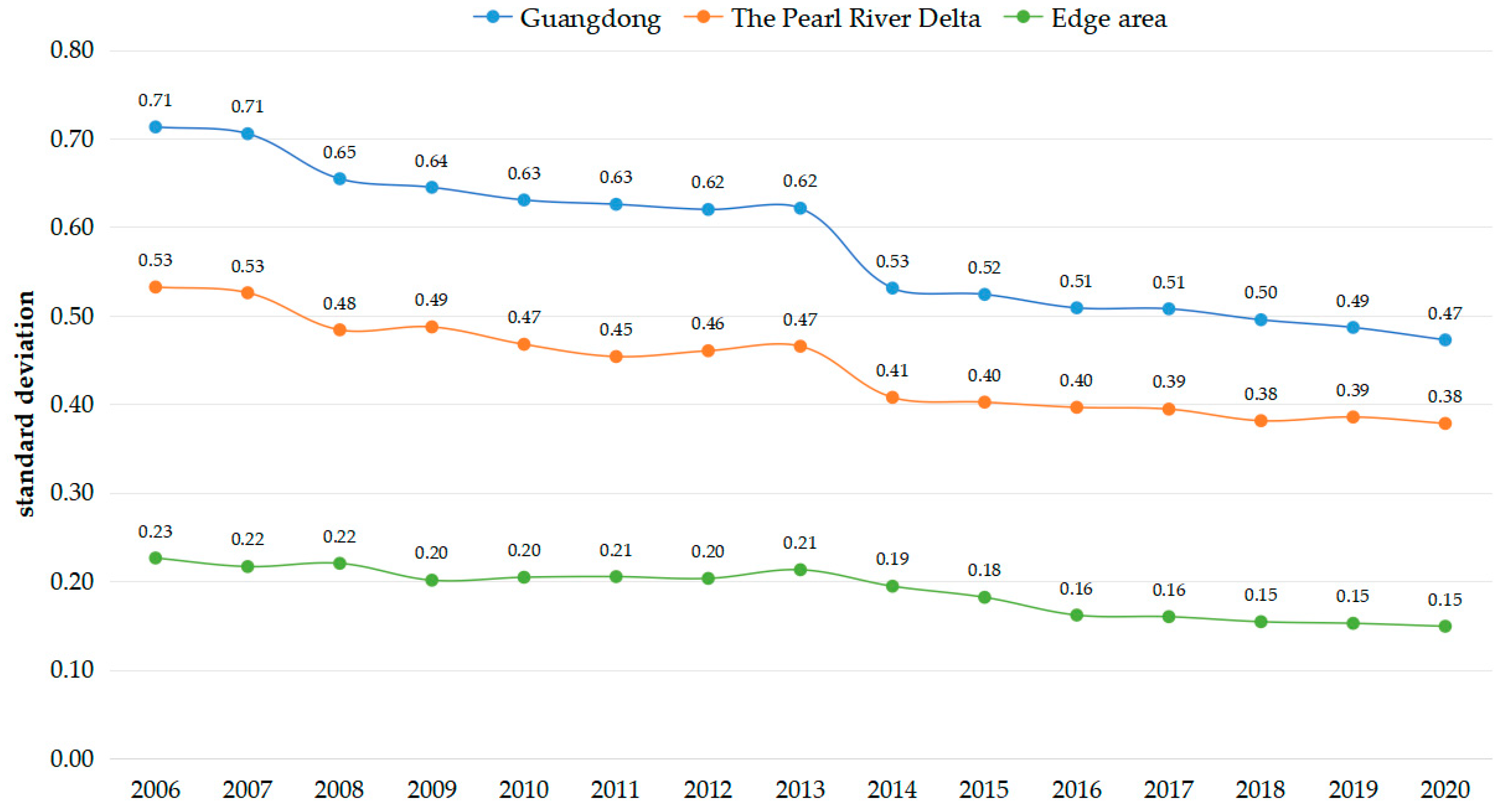
The standard deviation of per-capita GDP is used to reflect the $\sigma$-convergence of urban economy in different regions of Guangdong. From 2005 to 2020, the standard deviation coefficient (SD) of per-capita GDP continued to shrink, indicating that there is σ-convergence in Guangdong (Figure 2). In terms of regions, the convergence trend in the PRD and the edge area is similar to that of Guangdong. From 2005 to 2020, the SD values of the PRD and the edge area decreased by 30.45% and 35.02%, respectively. The SD of the PRD is larger, but the decline is smaller, while the edge area is the opposite. It can be seen that the urban disparities in the PRD are larger but the convergence speed is smaller, and the urban disparities in the edge area is smaller, but the convergence speed is faster.

• The selection of a spatial econometric model

Geoda 1.18 software was used to test the spatial autocorrelation of urban per-capita GDP in Guangdong from 2006 to 2020. The results show that the global Moran’s I of per-capita GDP in Guangdong’s cities is greater than 0.47, and the statistical $Z$ value is greater than 3.6, and all pass the 1% significance level test (

Table 3. Global Moran’s I of per-capita GDP.

Year	W1	W2	Year	W1	W2
2006	0.573 ***	0.619 ***	2014	0.499 ***	0.554 ***
	(4.6173)	(4.0579)		(4.0773)	(3.7112)
2007	0.583 ***	0.630 ***	2015	0.497 ***	0.557 ***
	(4.6808)	(4.1120)		(4.0594)	(3.7239)
2008	0.586 ***	0.631 ***	2016	0.487 ***	0.549 ***
	(4.6966)	(4.1173)		(4.0109)	(3.6924)
2009	0.558 ***	0.607 ***	2017	0.478 ***	0.540 ***
	(4.4956)	(3.9913)		(3.9405)	(3.6400)
2010	0.554 ***	0.603 ***	2018	0.484 ***	0.545 ***
	(4.4655)	(3.9841)		(3.9810)	(3.6684)
2011	0.556 ***	0.606 ***	2019	0.473 ***	0.539 ***
	(4.4924)	(4.0138)		(3.9076)	(3.6224)
2012	0.543 ***	0.591 ***	2020	0.476 ***	0.542 ***
	(4.3829)	(3.9216)		(3.9354)	(3.6397)
2013	0.532 ***	0.583 ***
	(4.3028)	(3.8647)

*** refer to significance at the 1% levels.

). It shows that the urban economy of Guangdong presents the distribution characteristics of spatial positive correlation, and there is spatial agglomeration between cities with similar per-capita GDP levels. The Moran’s I values of $W^1$ and $W^2$ showed a decreasing trend, indicating that the spatial agglomeration characteristics of the urban economy in Guangdong continued to weaken.

The urban economy in Guangdong presents a spatial positive correlation distribution feature, and if spatial factors are not taken into account when conducting convergence analysis, it may lead to bias in the results. Drawing on previous research [38] to select the model, we note the following: On the one hand, the LM and robust LM statistics of SAR and SEM were both significant at the 1% level (

Table 4. Conditional space β-convergence model test.

	Parameter	W1	W2
LM test	Moran’s I	3.258 ***	1.617 *
	LM-error	264.549 ***	354.191 ***
	Robust LM	63.724 ***	58.646 ***
	LM-lag	212.054 ***	334.217 ***
	Rubust LM	11.230 ***	38.672 ***
Hausman test	Hausman test	17.19 ***	8.54 ***
Wald test	Wald spatial lag	11.25 *	30.87 ***
	Wald spatial error	16.70 ***	16.96 ***

***, and * refer to significance at the 1%, and 10% levels.

), indicating that SDM has the best fitting effect. In addition, combining Hausman, it was found that the Walds statistics of SAR and SEM also passed the 10% significance test (Table 4), rejecting the hypothesis that the model can simplify. This means that the two spatial transmission mechanisms included in SDM cannot be ignored in terms of their impact on economic growth. The Hausman test results rejected random effects (Table 4), so we selected the SDM fixed effects model.

2.

Robustness testing

Using the time distance weight matrix ($W^2$) for spatial econometric analysis, the geographic distance weight matrix ($W^1$) was used in robustness tests for comparison. The results show that although there were some disparities in the size of the variable estimation coefficients, the direction and significance did not change fundamentally, in particular $\beta$ and $\rho$, which are always strongly significant (

Table 5. Absolute space β-convergence estimation results.

	W1	W2	PRD a	Edge Area a
$\beta$	−0.1334 ***	−0.0955 ***	−0.0918 ***	−0.1890 ***
	(−4.81)	(−4.49)	(−2.98)	(−4.27)
$W \times Y$	0.1062 ***	0.0620 ***	0.0586 **	0.1582 ***
	(3.59)	(2.78)	(1.87)	(3.50)
$\rho$	0.6766 ***	0.6688 ***	0.7369 ***	0.6437 ***
	(17.33)	(11.13)	(14.40)	(9.70)
Log-likelihood	572.3487	529.1923	240.0055	331.1577
Convergence speed ($\theta$)	0.41%	0.29%	0.22%	0.73%
Half-life ($\tau$)	167.21	238.51	314.49	95.57
${\mathrm{R}}^2$	0.2582	0.3033	0.2450	0.3017
$N$	294	294	123	168

^a using the time distance weighting matrix ($W^2$); numbers in parentheses are $t$ values; *** and ** refer to significance at the 1% and 5% levels.

and

Table 6. Conditional space β-convergence estimation results.

	W1	W2	PRD a	Edge Area a
$\beta$	−0.2817 ***	−0.4098 ***	−0.3412 ***	−0.4177 ***
	(−12.33)	(−12.29)	(−6.48)	(−8.23)
$lnR$	0.0157	0.0230 **	0.0366	0.0121
	(1.27)	(2.03)	(0.95)	(0.90)
$lnIP$	−0.0235	−0.0386 *	−0.2125 ***	−0.0178
	(−1.13)	(−1.85)	(−3.54)	(−0.89)
$lnInves$	0.0535 ***	0.0231 ***	0.0935 **	0.0562 ***
	(5.66)	(5.96)	(3.50)	(5.95)
$lnR\&D$	0.0064 **	0.0129 ***	0.0060	0.0093 **
	(3.50)	(3.92)	(1.41)	(2.15)
$lnFDI$	−0.0057	−0.0090 **	−0.0080	−0.0097 **
	(−1.52)	(−2.14)	(−1.08)	(−2.33)
$lnfiscal$	0.087 ***	0.1630 ***	0.1016 ***	0.0996 ***
	(4.08)	(7.55)	(3.53)	(3.12)
$W\times Y$	0.0741	0.0110	0.0016	0.1240
	(1.54)	(−0.11)	(0.02)	(1.24)
$W\times lnR$	−0.0016	−0.0213	−0.1649	−0.0052
	(−0.09)	(−0.56)	(−1.03)	(−0.21)
$W\times lnIP$	−0.0354 ***	−0.2124 ***	0.0306	−0.1514 **
	(−0.83)	(−2.85)	(0.31)	(−2.30)
$W\times lnInves$	−0.0376 **	0.0266	0.0577	0.0289
	(−2.24)	(0.48)	(0.72)	(0.75)
$W\times lnR\&D$	0.0105 **	0.0487 ***	−0.0054	0.0260 ***
	(2.11)	(3.07)	(−0.39)	(2.60)
$W\times lnFDI$	0.0006	0.0175	0.0242	0.0210
	(0.09)	(1.16)	(1.55)	(1.62)
$W\times lnfiscal$	−0.0129	−0.0307	−0.0091	−0.0100
	(−0.42)	(−0.50)	(−0.16)	(−0.14)
$\rho$	0.5946 ***	0.3658 ***	0.5891 ***	0.4381 ***
	(12.44)	(3.18)	(7.34)	(4.32)
$Log-likelihood$	610.2081	593.1951	268.9268	362.7365
$Convergence speed \left(\theta \right)$	0.96%	1.53%	1.21%	1.57%
$Half-life \left(\tau \right)$	72.36	45.40	57.37	44.27
${\mathrm{R}}^2$	0.2464	0.3036	0.6406	0.2872
$N$	294	294	126	168

^a using the time distance weighting matrix ($W^2$); numbers in parentheses are $t$ values; ***, **, and * refer to significance at the 1%, 5%, and 10% levels.

). These indicate that the model design of this study is feasible and the results are robust.

When using SDM for analysis, Wald statistic testing is required to demonstrate the applicability of the model. The Wald spatial lag and Wald spatial error statistics corresponding to the $W^1$ and $W^2$ both passed the significance test (Table 4), indicating that using SDM is appropriate.

3.

Space β-Convergence analysis

The test results of the absolute space β-convergence model are shown in Table 4. The $\rho$ corresponding to the two spatial weight matrices is significantly positive, which indicates that there is a significant positive spatial effect in Guangdong’s urban economy. The $\rho$ of $W^2$ is greater than $W^1$, indicating that economic spillovers between cities with close temporal distance is stronger than that of geographical distance.

The convergence coefficients of $W^1$ and $W^2$ are both significantly negative, indicating that there is absolute β-convergence in the per-capita GDP of Guangdong’s cities. The economically backward cities show a catch-up trend with the leading cities. According to Formula (14), the $\theta$ and $\tau$ can be calculated (Table 5). The convergence rate of $W^1$ and $W^2$ is between 0.29% and 0.41%, and the half-life year is between 167.21 and 238.51 years. This shows that the absolute convergence rate of per-capita GDP in Guangdong’s cities is relatively low, the half-life year is long, and the economic disparities will exist for a long time. A regional comparison shows that the absolute value of convergence coefficient and convergence speed in the edge area is larger than that in the PRD, and the half-life year is shorter. Therefore, the convergence trend in urban economic development disparities in the edge area is stronger than that in the PRD.

Overall, the per-capita GDP of Guangdong’s cities has an absolute convergence trend, but the convergence cycle is relatively long, and the current situation of unbalanced economic development will not change in a short period of time. There are disparities in the convergence of different regions, and the convergence trend in the edge area is stronger than that of the PRD.

Considering the influence of industrial agglomeration ($R$), industrial proximity ($IP$), investment ($\mathrm{Inves}$), $\mathrm{FDI}$, $\mathrm{R}\&\mathrm{D}$, and fiscal, the conditional space β-convergence model was used to test the spatial convergence of per-capita GDP in Guangdong. The results are shown in Table 5. The $\beta$ of $W^1$ and $W^2$ is significantly negative, and the absolute values are greater than the absolute space convergence (Table 5 and Table 6). It shows that when setting variables, the urban economy of Guangdong still has convergence, and the convergence intensity is greater. This once again proves the convergence of the urban economy in Guangdong. The convergence speeds ($\theta$) of $W^1$ and $W^2$ are 0.96% and 1.53%, respectively, and the half-life ($\tau$) is between 45.4 and 72.36 years (Table 6). The conditional convergence trend is stronger than the absolute convergence. Barro et al. (1991) considered a convergence rate of 2% and half-life year of 35 years to be typical features of cross-regional economic convergence research [42]. Wenqing P. (2010) calculated that the economic convergence rate of Eastern, Central and Western China is only 1.15%, and the catch-up cycle is 60.4 years [43]. The speed and period of conditional convergence in our study are close to the above research results, which indicates that the estimation results of the conditional β-convergence model are more robust and reliable. A regional comparison shows that the absolute values of $\beta$ and $\theta$ in the edge area are greater than those in the PRD, and the $\mathsf{\tau }$ is shorter, which again shows that the conditional convergence trend in the edge area is stronger.

In $W^2$, the regression coefficients of industrial agglomeration ($lnR$) are significantly positive, indicating that industrial agglomeration has positive externalities.Convenient transportation between cities can contribute to economic spillover. Hypothesis (H1a) is validated. The regression coefficient ($lnIP$) and spatial lag coefficient ($W\times lnIP$) of industrial proximity are significantly negative, indicating that industrial proximity has a negative impact on the local economy and the economic development of neighboring regions. Hypothesis (H3b) is validated. The regression coefficients of $lnInves$, $lnR\&D$, and $lnFiscal$ in Guangdong are all positive. Among them, the coefficient of $lnFiscal$ is the largest. It shows that investment, R&D and fiscal have a positive effect on urban economic convergence, and fiscal has the greatest effect. The coefficients of lnFDI are all negative, indicating that the growth of FDI is not conducive to Guangdong’s economic convergence. FDI is more profit-driven and often gathers in areas with superior geographical conditions and fast investment returns, resulting in higher spatial differentiation. Yang et al. (2015) demonstrated the positive impact of fiscal expenditure on economic development [37]. As an important means of government intervention in the economy, fiscal plays an important role in optimizing resource allocation and strengthening macro-control. The coefficients of lnInves and lnfiscal are larger in the PRD than in the edge area, indicating that investment and fiscal have a more positive impact on the economic convergence of the PRD. The coefficient of lnFDI is significantly negative in the edge area, but not significant in the PRD, indicating that FDI has a greater negative impact in the edge area. 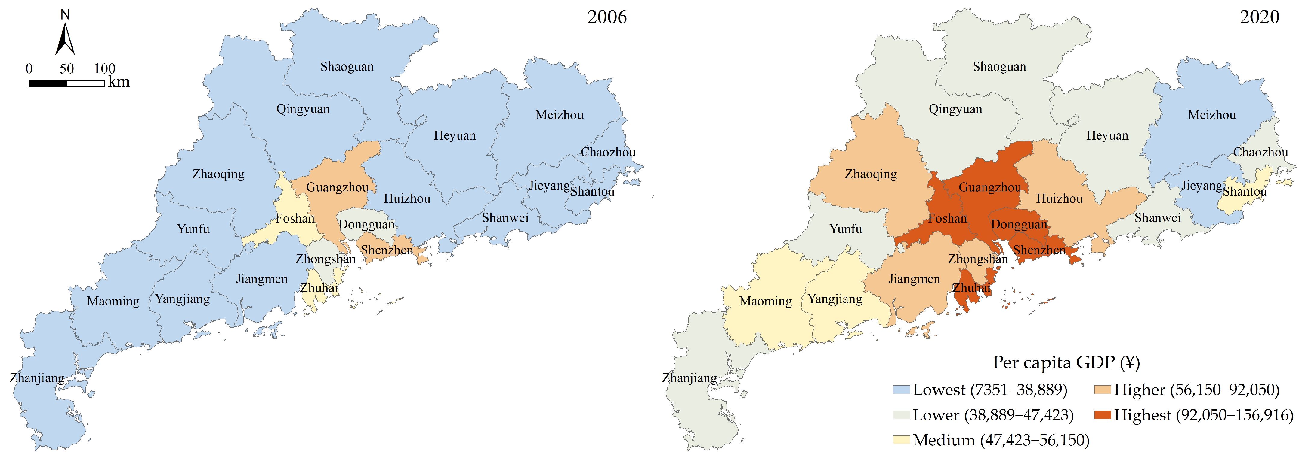As shown in Figure 1, there is a gradient difference in the economic level between the PRD and edge area, and the urban economic levels within the two regions are relatively similar. The coefficient of industrial agglomeration in the PRD and edge area is not significant, but it is significantly positive throughout Guangdong Province. This indicates that the “squeezing effect” generated by industrial agglomeration occurs between the PRD and edge area. The economic spillovers brought about by industrial agglomeration occur between regions with significant economic gradients, and hypothesis (H2) is validated.

6. Discussion

6.1. Understanding Regional Economic Disparities and Convergence

The per-capita GDP among Guangdong’s cities exhibits substantial variations, yet notable spatial convergence is observed. The phenomenon of economic convergence suggests that it is feasible to foster coordinated regional development and narrow the regional development disparity. The decomposition of the Theil index further indicates that the main source of the overall gap in Guangdong is the development gap between the PRD and the edge area. Consequently, the key to addressing the heterogeneity issue in Guangdong’s urban economic development is to narrow this gap. Fortunately, not only is there a convergent trend within the more developed PRD and the less developed edge area themselves, but the disparities between the two regions are also narrowing. In recent years, Guangdong Province has actively broken through the limitations of administrative divisions, experimented with cross-regional economic cooperation, and established many successful examples of an enclave economy [44,45], for instance, the Guangdong Shenshan Special Cooperation Zone, the Guangdong Shunde Qingyuan (Yingde) Industrial Park, and the industrial park jointly established by Jiangsu Sunan and Subei. The cooperation model of an “enclave economy” has achieved remarkable results in promoting coordinated regional development [46]. Therefore, there is no phenomenon of underdeveloped areas converging into the “poverty trap” in Guangdong’s economy. As one of the most unbalanced provinces in China’s regional development, Guangdong’s urban economy has maintained a spatial convergence trend over the past decade, demonstrating that China’s regional development model is uniquely inclusive.

6.2. The Spatial Spillover Effect and Economic Convergence

Cities serve as spatial platforms for human economic activities. The interplay among cities serves as a pivotal driving force in reducing regional development disparities and fostering coordinated regional development [47,48]. We incorporated factors such as geographical distance and spatial adjacency to provide a richer perspective on examining spatial spillover effects. Our research confirms that Guangdong’s urban economy has significant spatial spillover effects and convergence. Meanwhile, we found that regions with strong spatial spillovers do not necessarily have stronger convergence, as spatial convergence is not only influenced by spatial spillovers but also by economic factors. The spatial spillover effect of the PRD is stronger than that of the edge area, but the negative externalities brought about by industrial proximity in the region are also significantly stronger than those in the peripheral areas. Under the comprehensive influence of spatial effects and industrial proximity, the convergence speed of the PRD is weaker than that of the edge area.

6.3. The Impact of Industry on Economic Convergence

We used spatial econometric models to reveal the impact of industrial agglomeration and industrial proximity on Guangdong’s economic development, which is not easily discernible through traditional index methods. Industrial agglomeration and industrial proximity have both had significant impacts on economic convergence. Industrial agglomeration in the PRD region has already had a “crowding-out effect”. The “crowding out effect” triggers industrial migration and the flow of labor, capital, and other factors, resulting in economic spillovers to the surrounding areas, which is conducive to narrowing the regional development gap. However, the convergence of industrial structure shows a significant negative value, indicating that it has a hindering effect on economic growth. One potential reason is that the convergence of industrial structure can easily lead to vicious competition, which is not conducive to economic development. We further discovered regional differences in the impact of industrial proximity on the economy. The similarity of industries between cities in the PRD and other cities will have adverse effects on their own economic development, while the edge area will have adverse effects on the economies of other cities. This may be due to the central cities with obvious industrial advantages in the PRD, while competition in other cities is relatively weak. The specific reasons need further research in the future.

7. Conclusions

This study examined the spatial distribution characteristics and regional differences of the urban economy in Guangdong. Then, a spatial econometric model was constructed to analyze the convergence and influencing factors of Guangdong’s urban economy. The research conclusions are as follows:

(1) The spatial layout of Guangdong’s urban economy exhibits a pronounced “core-periphery” structure, with pronounced regional disparities. Although the gap between the PRD and edge area, as well as within the two regions, continues to narrow, the interval gap has always been the main source of the overall differences.

(2) The urban economic development in Guangdong Province exhibits both σ-convergence and β-convergence. The conditional β-convergence rate is approximately 1.52%, and the half-life is approximately 45 years. The PRD has a developed economy with significant disparities, but the convergence rate is relatively slow, while the edge area is the opposite.

(3) Industrial agglomeration has a positive effect on urban economic convergence, while industrial proximity has a negative spillover effect. There is spatial heterogeneity in the impact of industries on economic development. Industrial agglomeration has a positive impact on the overall economic development of Guangdong, but it is not significant within the regions. The convergence of industrial structure has significant negative externalities in the PRD region, and its impact is not significant in the edge area.

(4) Industrial agglomeration in the PRD generates economic spillovers to the surrounding areas, which is conducive to narrowing the regional development gap. However, the phenomenon of industrial proximity in Guangdong has brought about vicious competition, which has a negative impact on economic development. Therefore, local governments should fully leverage the positive spillover effects of industrial agglomeration. At the same time, attention should also be paid to solving the problem of industrial homogenization development.

This study not only provides empirical evidence for practical research on measuring regional differences and convergence, but it also serves as a beneficial supplement to the study of Guangdong’s economic convergence and its influencing factors. There are still some shortcomings: (1) As China is currently undergoing a pivotal period of economic transformation, compounded by challenges like an aging population and the global economic downturn leading to a contraction in exports, these factors will have profound implications for the evolution of regional economic growth patterns. Thus, it is imperative to incorporate additional factors to continuously monitor and unveil China’s regional economic patterns and convergence trends in the coming years. (2) Empirical testing of the impact of various types of inter-regional economic connections on regional economic convergence is lacking. This is a crucial aspect of future research.

References

1. Lee, B.S.; Peng, J.; Li, G.; He, J. Regional Economic Disparity, Financial Disparity, and National Economic Growth: Evidence from China. Rev. Dev. Econ. 2012, 16, 342–358. [Google Scholar] [CrossRef]
2. Wang, S.J.; Wang, Y.; Zhao, Y.B. Spatial spillover effects and multi-mechanism for regional development in Guangdong province since 1990s. Acta Geogr. Sin. 2015, 70, 965–979. [Google Scholar]
3. Fu, Q.; Li, S.W. Review of Research on Economic Convergence Theory Based on Economic Growth Theory. Inq. Into Econ. Issues 2016, 11, 161–172. [Google Scholar]
4. Xuebing, D.; Ruonan, C. Characteristics of the Temporal and Spatial Pattern of the Economic Disparity and Convergence Between Different Regions in China. Econ. Geogr. 2020, 40, 11–21. [Google Scholar]
5. Zeng, P.; Pang, Y. Regional Differences and Convergence Analysis of Economic Development in Chinese Urban Agglomerations. Stat. Decis. 2023, 39, 132–136. [Google Scholar]
6. Lu, M.; Li, P. Coordinated development between urban and rural areas and regions. Econ. Res. J. 2022, 57, 16–25. [Google Scholar]
7. Pengfei, L.; Ming, L. Urban Systems: Understanding and Predicting the Spatial Distribution of China’s Population. China World Econ. 2021, 29, 35–62. [Google Scholar]
8. Gege, C.; Teng, L.; Weiqi, L. Producer Services Agglomeration, Spatial Spillover and Urbanization: From the Perspective of New Economic Geography. Front. Sci. Technol. Eng. Manag. 2022, 41, 76–82. [Google Scholar]
9. Bindong, S. Highlighting the Scientific Concept in the Future Spatial Planning. Frontiers 2020, 4, 81–88. [Google Scholar]
10. Helsley, R.W.; Strange, W.C. Coagglomeration, clusters, and the scale and composition of cities. J. Political Econ. 2014, 122, 1064–1093. [Google Scholar] [CrossRef]
11. Feng, Q.; Guoping, Z.; Heng, Z. Research on Problem of Industrial Structure in the Yantse River Delta. China Ind. Econ. 2005, 4, 77–85. [Google Scholar]
12. Hong, D. Spatial Spillover Effects of Industrial Isomorphism on Regional Economic Growth—Taking the Beijing-Tianjin-Hebei Region as Example. J. Cap. Univ. Econ. Bus. 2021, 23, 44–54. [Google Scholar]
13. Liu, X.; Wang, N.; Ji, X. Siphon Effect of Central Cities and Coordinated Development of Regions. China Soft Sci. 2022, 4, 76–86. [Google Scholar]
14. Dachun, F.; Mengdi, P. Research on the Characteristics of Network Structure of Isomorphism in China’s High-tech Industry. Contemp. Econ. Manag. 2020, 42, 59–65. [Google Scholar]
15. Fuzhuo, F. An Improved Method of Measuring Industrial Structure Similarity Degree between Areas. J. Quant. Technol. Econ. 2013, 7, 98–115. [Google Scholar]
16. Chen, L.; Liu, X. A Study on the Converging Evolution of Industrial Structure among Cities in the Yangtze River Delta Region and Its Influencing Factors. J. Soochow Univ. (Philos. Soc. Sci. Ed.) 2023, 44, 55–66. [Google Scholar]
17. Krugman, P. The role of geography in development. Int. Reg. Sci. Rev. 1999, 22, 142–161. [Google Scholar] [CrossRef]
18. Sergio, J.R.; Montouri, B.D. US Regional Income Convergence: A Spatial Econometric Perspective. Reg. Stud. 1999, 33, 143–156. [Google Scholar]
19. Abreu, M.; de Groot, H.L.F.; Florax, R.J.G.M. Space and Growth: A Survey of Empirical Evidence and Methods. SSRN Electron. J. 2004, 21, 13–44. [Google Scholar] [CrossRef]
20. Pfaffermayr, M. Conditional β- and σ-convergence in space: A maximum likelihood approach. Reg. Sci. Urban Econ. 2009, 39, 63–78. [Google Scholar] [CrossRef]
21. Yin, Y.; Yaoqi, T. From Industrial Convergence to Industrial Clusters: A New Structural Economics Analysis of the Manufacturing Industry in the Yangtze River Delta. J. Hohai Univ. (Philos. Soc. Sci.) 2022, 2, 45–52. [Google Scholar]
22. Wu, Y.; Zhu, X. Industrial policy and economic geography: Evidence from China. J. Asia Pac. Econ. 2016, 22, 173–190. [Google Scholar] [CrossRef]
23. Zhang, H.; Sun, T. Network Externalities of Urban Economic Growth in Chinese Urban Agglomerations and the Mechanism. Res. Econ. Manag. 2022, 43, 48–64. [Google Scholar]
24. Yu, D.; Zhang, K. Factor Market Segmentation, Convergence of Industrial Structure and Advanced Development of Manufacturing Industry. Res. Econ. Manag. 2020, 41, 36–47. [Google Scholar]
25. Peilin, D.; Bingxin, Z. The Convergence Evolution and Spatial Pattern of Regional Industrial Structure from the Perspective of K-cores. Inq. Into Econ. Issues 2014, 11, 87–93. [Google Scholar]
26. Wenjie, Z.; Bao, S. Created unequal: China’s regional pay inequality and its relationship with mega-trend urbanization. Appl. Geogr. 2015, 61, 81–93. [Google Scholar]
27. Theil, H.; Scholes, M. Forecast evaluation based on a multiplicative decomposition of mean square errors. Econom. Soc. 1967, 35, 70–88. [Google Scholar] [CrossRef]
28. Hengmei, G.; Xiaodong, M. Evolution of Economic Spatial Pattern and Centrality Measure of Huaihai Economic Zone Based on Night-Time Light Data. Geogr. Geo-Inf. Sci. 2020, 36, 34–40. [Google Scholar]
29. UNIDO. World Industry Since 1960: Progress and Prospects; United Nations: New York, NY, USA, 1979. [Google Scholar]
30. Friedman, M. Do Old Fallacies Ever Die? J. Econ. Lit. 1992, 4, 229–2132. [Google Scholar]
31. Xie, H.; Wang, W. Spatiotemporal differences and convergence of urban industrial land use efficiency for China’s major economic zones. J. Geogr. Sci. 2015, 25, 1183–1198. [Google Scholar] [CrossRef]
32. Ramsey, F.P. A Mathematical theory of Saving. Econ. J. 1928, 38, 543–559. [Google Scholar] [CrossRef]
33. William, J.B. Productivity Growth, Convergence, and Welfare What the Long-Run Data Show. Am. Econ. Rev. 1986, 5, 1072–1085. [Google Scholar]
34. Melvyn, W.; Yao, J.Y. Provincial Conditional Income Convergence in China, 1953–1997: A Panel Data Approach. Econom. Rev. 2007, 22, 59–77. [Google Scholar]
35. Houkai, W. Effects of Foreign Direct Investment on Regional Economic Growth in China. Econ. Res. J. 2002, 4, 19–26. [Google Scholar]
36. Katircioglu, S.; Fethi, S.; Caner, H. Testing the Higher Educationled Growth Hypothesis in a Small Island: An Empirical Investigation from a New Version of the Solow Growth Model. Qual. Quant. 2014, 2, 729–744. [Google Scholar] [CrossRef]
37. Yang, W.; Fidrmuc, J.; Ghosh, S. Macroeconomic effects of fiscal adjustment: A tale of two approaches. Int. Money Financ. 2015, 57, 31–60. [Google Scholar] [CrossRef]
38. Bai, J.; Wang, Y.; Jiang, F.; Li, J. R&D Element Flow, Spatial Knowledge Spillovers and Economic Growth. Econ. Res. J. 2017, 52, 109–123. [Google Scholar]
39. López-Bazo, E.; Vayá, E.; Mora, A.J.; Suriñach, J. Regional economic dynamics and convergence in the European Union. Ann. Reg. Sci. 1999, 33, 343–370. [Google Scholar] [CrossRef]
40. Andrés, R.P.; Fratesi, U. Between development and social policies: The impact of European structural funds in objective regions. Reg. Stud. 2004, 38, 97–113. [Google Scholar]
41. Dawson, J.W.; Strazicich, M.C. Time-series tests of income convergence with two structural breaks: Evidence from 29 countries. Appl. Econ. Lett. 2010, 17, 909–912. [Google Scholar] [CrossRef]
42. Barro, R.J.; Sala-i-Martin, X.; Blanchard, O.J.; Hall, R.E. Convergence across States and Regions. In Brookings Papers on Economic Activity; Brookings Institution: Washington, DC, USA, 1991; pp. 107–182. [Google Scholar]
43. Wenqing, P. Regional Economic Differences and Convergence in China. Soc. Sci. China 2010, 1, 72–84+222–223. [Google Scholar]
44. Hangjun, H.; Jingxiang, Z. Innovation-Driven Reverse Enclaves: The Cross-Gradient Innovation Development. Plan. Stud. 2022, 46, 30–39. [Google Scholar]
45. Xuan, W.; Kuai, Y. The Governance Logic of Enclave Economy in Terms of the Spatial Production: A Case Study of Shenzhen-Shanwei Special Cooperation Zone. Chin. Public Adm. 2021, 2, 76–83. [Google Scholar]
46. Li, M.; Huang, Z. “Enclave Economy” for Promoting Regional Coordinated Development: Development Mode and Future Trend. Tianjin Soc. Sci. 2020, 4, 97–102. [Google Scholar]
47. Benjamin, D.; Brandt, L.; Giles, J. Did Higher Inequality Impede Growth in Rural China? Econ. J. 2011, 121, 1281–1309. [Google Scholar] [CrossRef]
48. Guoxin, L.; Junkuang, W.; Yao, C. Innovation incentives and R&D spillover. Chin. J. Manag. Sci. 1999, 7, 68–75. [Google Scholar]
Figure 1. Spatial distribution of urban per-capita GDP in Guangdong.
Land 13 00073 g001
Figure 2. The standard deviation of urban economy in different regions.
Land 13 00073 g002