Complex Methodology for Spatial Documentation of Geomorphological Changes and Geohazards in the Alpine Environment

Abstract

The alpine environment with a high degree of nature protection is characterized by complete non-intervention. The processes and phenomena occurring in it are exclusively of a natural origin. Related geohazards are threatening the safety of people’s movement. They arise as a result of a combination of meteorological, hydrological, and geological–morphological factors permanently operating in the country. Therefore, the prevention of fatal events is limited to monitoring and predicting changes in selected objects where we expect change. Changes in the shape and dimension, or the object’s deformation, can be documented using geodetic and photogrammetric measurements. Our research focuses on monitoring a rock talus cone in High Tatras, Slovakia, at an altitude of 1700 m above sea level (ASL), created mainly due to erosion and seasonal torrential rains. To monitor changes in selected objects, we used mass non-contact methods of terrestrial laser scanning (TLS), UAS photogrammetry based on the principle of structure-from-motion–multi-view stereo (SfM–MVS), and airborne laser scanning (ALS). From the selective measurement methods, spatial measurement by a total station (TS) and height measurement based on the principle of precise leveling were used in the monitoring deformation network on a stand-alone boulder. The research results so far analyze and evaluate the possibilities, limits, effectiveness, and accuracy of the measurement and data processing methods used. As a result, we propose a complex methodology for monitoring similar phenomena in alpine environments.

1. Introduction

Collecting spatial data using non-contact methods is possible using modern technology, which consists of sensors of various types with appropriate methodology. These methods are efficient and accurate, allowing us to obtain a large amount of data in a short time without the need for direct contact with the measured object. The current trend in the use of non-contact technologies is their use for monitoring hard-to-reach areas, objects, or phenomena. Non-contact methods are also effectively used to monitor geohazards, natural processes, or the development of changes in the landscape in an alpine environment. The alpine environment is specific due to its georelief, climatic conditions, and natural processes, which are triggered by climatic and temperature influences such as water, snow, frost, or sunshine. Due to these indicators, tracking the changes and dynamics of the georelief is very demanding from both technical and financial aspects. However, progress in data collection using non-contact methods [1,2] enables more efficient, accurate, and simple terrain monitoring in alpine environments. The advantage of non-contact methods is that they can capture a large area of the Earth’s surface relatively quickly with high accuracy and provide digital terrain models, point clouds, aerial photographs, or orthophoto maps [3,4].

Photogrammetric and TLS methods are the most commonly used non-contact methods in alpine environments because the measurement in the field is carried out without direct contact with the object or the Earth’s surface. TLS measurement consists of surveying the shape and size of a scanned object or surface. As a result, a set of surveyed points (point cloud) is obtained, while data of every point contains a spatial coordinate and a value of the reflected beam’s intensity [5]. High-quality panoramic images are taken during measurement, which partially serves to color the scanned points. In most cases, it is necessary to survey from several instrument positions. This is due to the size of the scanned area, the complexity of the object, and the required level of detail in the scan. Care must be taken when choosing the next scanning position to ensure that individual scans are sufficiently overlapped for successful mutual registration [6]. TLS, using the reflection of electromagnetic radiation, enables the recording of the 3D geometry of objects and landscape relief with high accuracy and detail in a short time [7,8]. Another method for collecting data in an alpine environment is aerial photogrammetry. In photogrammetry, the task is to convert information from the central projection of the image to the orthogonal projection. The photogrammetric method SfM–MVS is one of the most modern and advanced procedures in the photogrammetric processing of captured images [9,10,11]. The SfM–MVS method’s main principle is estimating a spatial object’s three-dimensional structure based on two-dimensional images from a moving camera [12,13].

In recent years, the novelty has been applying the method of close-range aerial photogrammetry, where the camera is mounted on a remotely piloted or autonomous aerial carrier called an unmanned aerial system (UAS) [14]. UASs are preferred, especially in smaller areas, due to their ease of use and low acquisition costs. The advantages of using a UAS are the shortening of fieldwork time and speed of photogrammetric data collection with processing, resulting in high detail and accuracy of terrain models. Terrain models generated by modern software have become a suitable non-contact method regarding quality results and measurement efficiency [15,16]. Nowadays, UASs make it possible to capture the Earth’s surface with an improvement in the level of detail at the same flight height above ground level (AGL), reducing the required number of images and thus the flight time and cost of imaging [17,18,19]. In an alpine environment, it is also possible to use Lidar (light detection and ranging) technology, which can be characterized as optical, modern, and progressive technology for remote sensing of the Earth. The advantage of this method is the achievement of a high-resolution point cloud. The use of Lidar technology is addressed in many publications [20,21,22,23]. National campaigns in Slovakia, the Czech Republic, Austria, and Germany are also dedicated to Lidar technology, which uses ALS to document entire countries [24] by comprehensive digital elevation models (DEM). Non-contact methods can quickly capture many irregular objects in high detail and accuracy, which is their advantage over classical geodetic techniques. However, classical geodetic methods such as total station surveying or GNSS (global navigation satellite system) surveying are used to determine the coordinates of ground control points (GCPs). GCPs are used for georeferencing and are designed to be clearly visible in images [25,26]. Georeferencing involves the process of transforming image coordinates to ground coordinates through GCP. The number, distribution, and accuracy of GCPs affect the accuracy of georeferencing. In cases where GCP stabilization is not possible, it is recommended to use a UAS with an on-board GNSS RTK/PPK module, where each image is assigned a precise position and georeferencing by GCPs is not necessary [27,28,29].

Geodetic and geological monitoring, analyzing, and predicting landslides, shifts and changes in the landscape’s development, and georelief are also important in the alpine environment. The staged measurements can determine changes in the position of objects, the morphology of landslides, and the shape of the terrain [30]. After the base measurement, another measurement is taken, either at a predetermined period or after a significant event, and the differences between the two epochs are subsequently analyzed. Displacements or shifts, especially their vertical component, can be determined by various physical measurement methods, such as mechanical, optical, electrical, electronic, and hydrostatic methods. Geodetic methods are commonly used, especially leveling [31,32], trigonometric methods [33], hydrostatic leveling, and photogrammetric methods.

This article summarizes the possibilities of monitoring spatial changes in the specific alpine environment in a small-scale area. Our research is focused on the methodology of spatial data collection in a specific alpine terrain using selected methods with their mutual comparison. We analyze results based on proven surveying methods and technologies available to a wide range of scientists and practical users. As a result, we show that these methods bring high work efficiency, are economically acceptable, and achieve significant quality in terms of accuracy and detail of obtained data. An important factor is also the fast repeatability of measurements, which can have a practically daily frequency if necessary. This research is intended to devise a comprehensive methodology with results that can be generalized for scientific and practical purposes in areas of a similar nature and scope.

2. Study Area

The Small Cold Valley, located in the northern part of the Slovak Republic, in the Prešov region, in the village of Vysoké Tatry, was chosen as the study area in this article. It is a terraced valley with a length of 4.5 km, which has been under the management of the Tatra National Park (TANAP) with five levels of protection since 1948. The Small Cold Valley belongs to the highest, fifth level of protection. Since 1993, it has been included in the international list of UNESCO biosphere reserves. The area of TANAP is 73,800 hectares, on which there are 25 peaks above 2500 m above sea level. The highest is Gerlachovský štít, with an altitude of 2655 m ASL. The geomorphological division of the territory of Mala Studena dolina is described in

Table 1. Characteristics of the study area Small Cold Valley.

Territorial Classification
Region	Prešov
District	Poprad
Village	Vysoké Tatry
Cadastral area	Tatranská Lomnica
Geomorphological classification
Geomorphological system	Alps–Himalaya System
Geomorphological sub-system	Carpathian Mountains
Geomorphological province	Western Carpathians
Geomorphological sub-province	Inner Western Carpathians
Geomorphological area	Fatra-Tatra Area
Geomorphological unit	Tatra Mountains
Geomorphological sub-unit	Eastern Tatras
Geomorphological part	High Tatras
Regional geological division	Fatra-Tatra zone

[34].

The Small Cold Valley (Figure 1) is located between the Lomnické Saddle, which borders the eastern side, and the Prostredný Ridge, which separates it from the Large Cold Valley on the west. At the end of the Small Cold Valley, below the Ľadový Peak massif (2627 m ASL), there is the Basin of the Five Spišské ponds, and The Small Cold Stream crosses the valley [35]. The Small Cold Valley stretches from the Studené streams’ confluence to the High Tatras’ main ridge. The lower, approximately 130 m high rock threshold lies just below the forest line at an altitude of 1330–1460 m ASL. It is called the Schodíky. The grassy forest glade above Schodíky, at the beginning of its own valley, just to the east of the Small Cold stream, is called Malá Lomnická Garden. The lower part of the valley is dammed by a moraine rampart, behind which is a vast plain covered with grass and rhododendrons at an altitude of 1620–1700 m ASL called Veľká Lomnická Garden. Above this plain rises a prominent valley terrace approximately 200 m high, the Jazerná Wall, above which there are separate valley parts: the Basin of the Five Spišské ponds. There is a Great Hang and a Small Hang in the Jazerná Wall. In the upper part of the valley, above the Great Hang, is the well-known Téryho cottage (2015 m ASL) [35,36,37].

High mountain terrain with specific georelief and climatic conditions supports a wide range of natural processes with various morphodynamic phenomena. Various influences, including water, sunshine, snow, frost, and temperature changes, are reflected in the spatial occurrence and intensity of morphological processes. Many of these processes occur in the highest positions of ridges and peaks; others affect the slopes of valleys. The entire study area has several geomorphological formations with debris flows and currents. These can be classified as geohazards since they cross frequent high-mountain hiking trails. Various falls of rock blocks, rock collapses, talus cones, or avalanche falls occur. These geohazards can be observed mainly on the valley’s side and rock walls. Talus cones are accumulation zones for material washed out of steep gullies. Stone blocks and boulders are common in the Small Cold Valley [38,39].

In the Small Cold Valley, the area at its end, which is located under the western wall of Lomnický Peak, at an altitude of approximately 2200 m ASL, with a geographical position of 49.186° N and 20.208° E, was chosen for this research. The accumulation area, where stones and debris are collected, is approximately 1600 m ASL. The total length of the research area is approximately 400 m. Rock size in the area ranges from a few centimeters to approximately 5 m. The width of the accumulation zone ranges from 20 m in its upper part to 80 m in its lower part. The site of this research is only accessible via a hiking trail.

3. Materials and Methods

In the research location in the Small Cold Valley, base and stage measurements were carried out between June 2018 and June 2022. The measurement methods and surveying devices are shown in

Table 2. Used measurement methods and measuring devices in individual epochs.

Measuring Device	Epoch
Spatial polar method
Leica TS 02	2018
Leica TS06	2022
GNSS method
GNSS set Leica GPS900cs	2018
GNSS set Leica GS07	2022
Photogrammetric method 20 megapixelov
UAS DJI Phantom 4 Pro	2018
DJI Phantom 4 RTK UAS	2022
TLS method
Leica P40	2018
Leica RTC360	2022
Leveling method 15.2 V
Leica DNA03	2022

.

Using the mentioned methods, it is possible to document the site’s current state, capture the terrain morphology in detail, and generate a digital terrain model (DTM), digital surface model (DSM), or DEM. The work was carried out in the field according to the following procedure (Figure 2):

• Terrain reconnaissance.
• Stabilization and surveying of fixed points of the geodetic reference network.
• Measurement of GCP coordinates for photogrammetry and TLS.
• Preparatory work and pre-flight preparation.
• Measurement by photogrammetric and TLS methods.
• Control and verification measurement.

3.1. Stabilization and Surveying of the Geodetic Network

In the first stage of measurement in June 2018, it was necessary to build a precise geodetic network, which formed the basis for other measurement methods. The precise geodetic network was formed by 7 permanently stabilized points located outside the survey area. Four geodetic network points were stabilized with stainless steel pins (Figure 3a), drilled into the rock, and fixed with Fischer chemical mortar. The three points of the geodetic network were stabilized by retro-reflective targets in the form of reflective foils (Figure 3b) stuck to large and compact stone blocks using a special Pattex Chemoprén Universal adhesive (Schwarzkopf & Henkel, Düsseldorf, Germany).

The geodetic network also included three temporarily stabilized points, measured using the GNSS method. These three points were used to connect the precise geodetic network to standard reference systems: Datum of Uniform Trigonometric Cadastral Network (S-JTSK) and Baltic Vertical Datum after adjustment (Bpv).

The temporarily stabilized points of the geodetic network were measured using the GNSS set Leica GPS900CS using the RTK (real-time kinematic) method with connection to the Slovak Real-time Positioning Service (SKPOS). The GNSS set Leica GPS900CS was placed in a stand during the measurement. Measurement at every point took 5 min, and the temporarily stabilized points of the geodetic network reached an accuracy of up to 2.0 cm in position and up to 4.0 cm in height. Permanently stabilized points of the precise geodetic network were measured in the first epoch using a Leica TS02 total station with a value of horizontal and zenith angle measurement accuracy of 7″ (0.0020 gon) and a distance measurement accuracy of 1.5 mm + 2 ppm. Each point of the geodetic network was measured in two faces of the telescope and three groups to achieve high measurement accuracy, reaching a standard deviation of up to 0.3 cm at each point. In the second epoch in 2022, a Leica TS06 total station was used to measure the geodetic network. A precise geodetic network was supplemented with three newly built points, which were stabilized like in the first measurement epoch. A comparison of the parameters of both total stations is shown in

Table 3. Comparison of technical parameters of Leica TS02 and Leica TS06 total stations [40,41].

	Leica TS02	Leica TS06
	Angle measurement
Accuracy	7″ (2.0 mgon)	2″ (0.6 mgon)
Compensator	Dual-axis	Dual-axis
	Distance measurement with a prism
Range	3–500 m	3–500 m
Accuracy	Standard: 1.5 mm + 2 ppm Fast: 3.0 mm + 2 ppm Tracking: 3.0 mm + 2 ppm	Standard: 1.5 mm + 2 ppm Fast: 3.0 mm + 2 ppm Tracking: 3.0 mm + 2 ppm
Standard measurement time	1.0 s	1.0 s
	Distance measurement without a prism
Range	>400 m	>500 m
Accuracy	2 mm + 2 ppm	2 mm + 2 ppm
Laser dot size	at 30 m: 7 × 10 mm at 50 m: 8 × 20 mm	at 30 m: 7 × 10 mm at 50 m: 8 × 20 mm
	Operation
Temperature range	−20 °C to +50 °C	−20 °C to +50 °C

. The position of permanently and temporarily stabilized points of the precise geodetic network is shown in Figure 4.

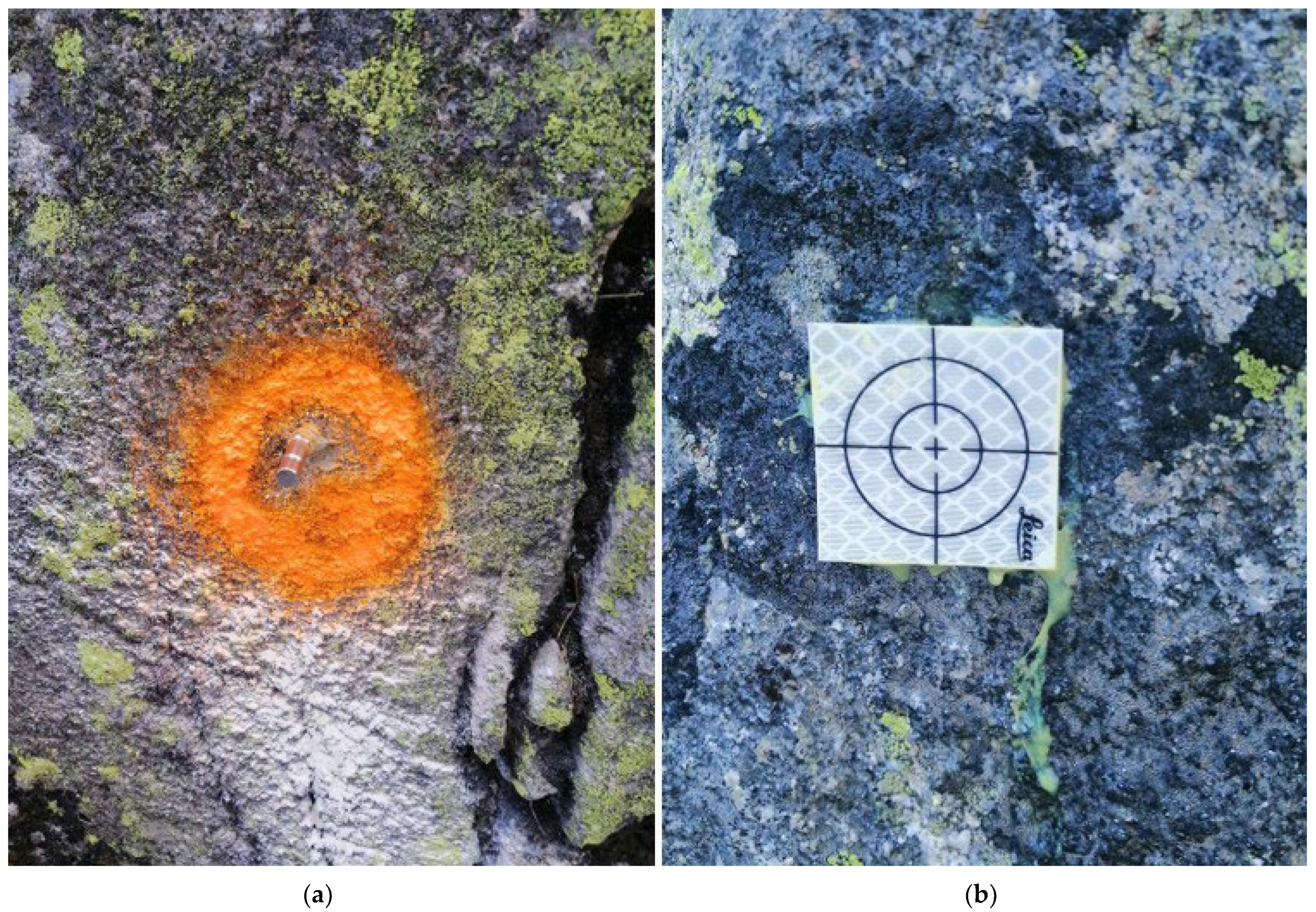
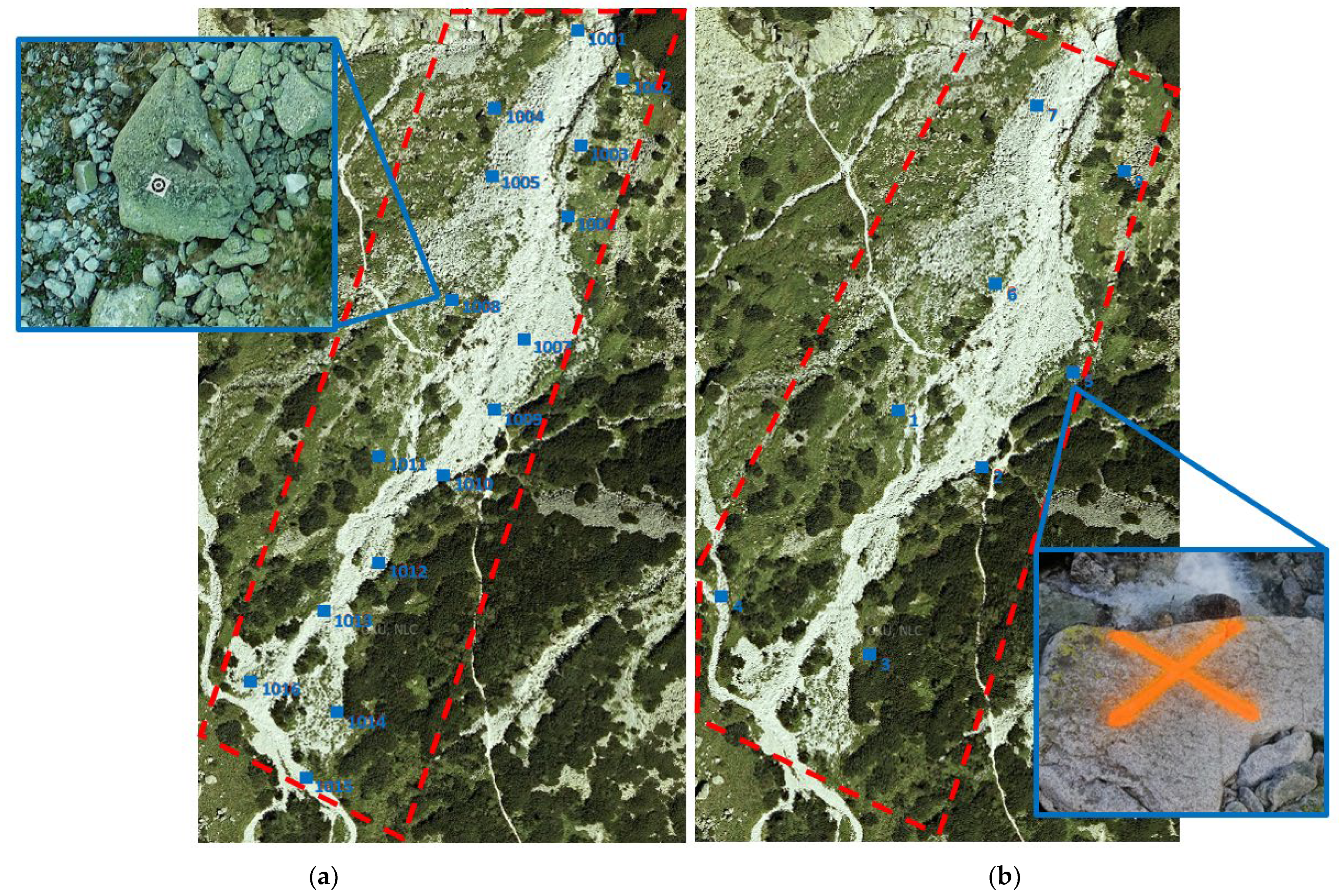
3.2. Surveying of GCP for Photogrammetry and TLS

In the first epoch in 2018, 16 black-and-white 12-bit targets with dimensions of 0.3 × 0.3 m were chosen as GCPs for photogrammetry, which were temporarily stabilized and placed around the talus cone (Figure 5a). GCP coordinates for photogrammetry were determined using the spatial polar method by the Leica TS02 (Leica Geosystems AG, Heerbrugg, Switzerland) total station (Figure 6a) in two groups of measurement. In the second epoch, 8 GCPs for photogrammetry (Figure 5b) were stabilized and evenly spaced using orange spray paint. The red line marks the boundaries of flight missions. The coordinates of GCPs were determined by a fast static method using the GNSS set Leica GS07 (Figure 6b). The estimated accuracy of GCP coordinate determination was 0.02 m in position and 0.04 m in height.

In the first epoch in 2018, the talus cone was also surveyed using the TLS method. As GCP for TLS, 14 black and white magnetic circular rotating Leica GZT21 HDS 4.5″ targets were used, which were evenly deployed over the scanning area (Figure 7). At least 3 GCPs for TLS were scanned from each position and used for mutual scan registration and georeferencing of TLS measurements. To determine the coordinates of the GCP points for TLS, a spatial polar method was used with a prismless measurement using a Leica TS02 total station with two repetitions of measurement.

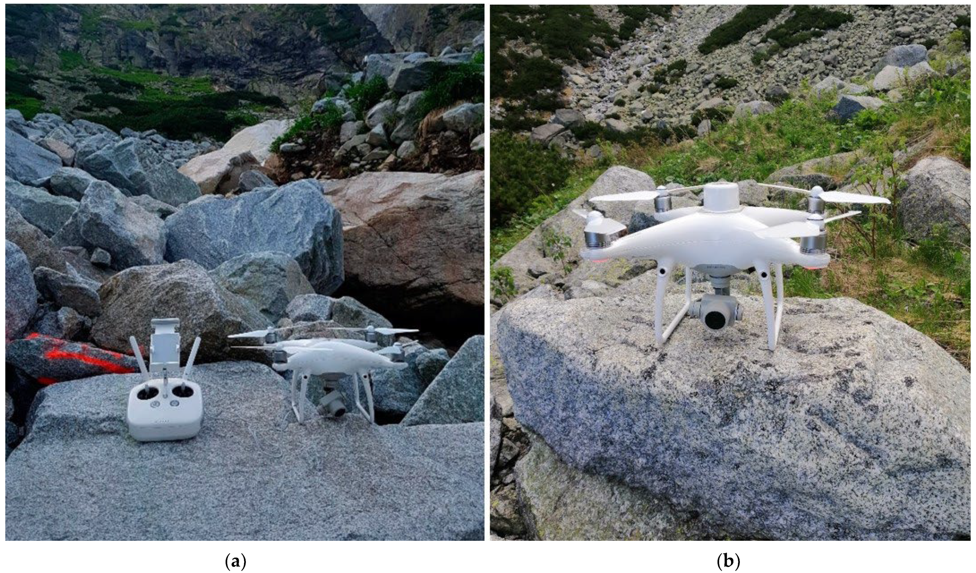
3.3. Measurement by Photogrammetric Methods

Photogrammetric surveying of the talus cone was carried out in 2018 using the UAS DJI Phantom 4 Pro (Figure 8a) equipped with a digital camera with a 20 Mpix CMOS sensor and a resolution of 5472 × 3648 pixels in automatic mode with a fixed ISO (100). Other technical parameters are shown in

Table 4. Comparison of technical parameters of UAS DJI Phantom 4 Pro and DJI Phantom 4 RTK [42,43].

	DJI Phantom 4 Pro	DJI Phantom 4 RTK
	Aircraft
Weight	1388 g	1391 g
Max ascent/descent speed	6 m/s and 4 m/s	6 m/s and 3 m/s
Max flight speed	20 m/s (mode S)	16 m/s (mode A)
Satellite positioning system	GPS/GLONASS	GPS/GLONASS/Galileo/BeiDou
Max flight time	28 min.	30 min.
Wind speed resistance	10 m/s
Operating temperature range	0 °C to +40 °C
	Camera
Sensor	1″ CMOS
Effective pixels Active pixels	20 Megapixels
Image size	4864 pixels × 3648 pixels (4:3)
Gimbal pitch	−90° to +30°
	GNSS Positioning Accuracy
Horizontal	up to 5 m (without augmentation service)	1 cm + 1 ppm (RTK)
Vertical		1.5 cm + 1 ppm (RTK)
	Battery
Type	LiPo 4S	LiPo 4S
Capacity	5350 mAh	5870 mAh
Voltage	15.2 V	15.2 V

. The flight plan was made in the Pix4D Capture application, which in 2018 could only perform automatic flights in a horizontal position. Therefore, 1389 images in the first epoch were acquired during four separate flights, which lasted approximately 3 h. Three flights were performed automatically with partial overlap at a flight height of 35 m AGL. Elevation between the upper and lower parts of the talus cone was 100 m, so each flight captured a different part of the cone. The first flight captured the upper part of the talus cone, the second documented the middle part, and the third covered the cone’s lower part. The fourth flight tried to capture the entire area of the talus cone in three bands with the camera oriented against the slope using manual piloting of the UAS at a flight height of up to 30 m above the ground. The first measurement epoch’s ground sampling distance (GSD) reached a 0.95 cm/pix value.

In the second epoch in 2022, a UAS DJI Phantom 4 RTK (Figure 8b) equipped with a camera with the same parameters was used for photogrammetric imaging of the researched area. Other technical parameters of UAS DJI Phantom 4 RTK are shown in Table 4. The advantage of this UAS is that it includes an on-board GNSS RTK receiver that can ensure centimeter accuracy of coordinates, which is significantly higher than the UAS used in 2018. Another advantage is that in 2022, the DJI GS RTK application was used for flight planning. Using this application, we can achieve a constant flight height over the terrain of different slopes or shapes. Using the Terrain Awareness mode strategy, flight trajectory was defined considering a generalized terrain model from epoch 2018. Therefore, in 2022, only one flight with a flight height of 45 m AGL was carried out. In total, 605 images with a GSD of 1.5 cm/pix were captured.

Parameters of flights in both epochs are shown in

Table 5. Comparison of flight parameters in both measurement epochs.

	DJI Phantom 4 Pro	DJI Phantom 4 RTK
Epoch of measurement	2018	2022
Number of images	1389	605
Number of GCP	16	8
Number of control points	10	5
Flight height [m]	35	45
GSD [cm/pix]	0.95	1.50
Overlap of the image [%]	80	70
Roll angle of the camera [°]	90	30
Pitch value of the gimbal [°]	75	80
Total flight time [h]	3	1

. In both epochs, a double-grid pattern of the flight scheme was used, where one flight line is perpendicular to the slope while the second flight line is in the direction of the slope.

3.4. TLS Measurement

In the first epoch of measurement in 2018, the TLS method was applied using a 3D terrestrial laser scanner, Leica ScanStation P40 (Figure 9). Selected technical parameters are listed in

Table 6. Technical parameters of terrestrial laser scanner Leica ScanStation P40 [44].

Type	Compact, pulse, time-of-flight, Laser class 1
Tilt compensator	Dual-axis
Scan rate	Up to 1,000,000 points/s
Accuracy	Distance: 1.2 mm + 10 ppm
	Angular:	horizontal: 8″
		vertical: 8″
	3D position: 3 mm at 50 m; 6 mm at 100 m
Target acquisition	2 mm standard deviation at 50 m
Range and reflectivity	Minimum range: 0.4 m
	Maximum range:	120 m @ 8% reflexivity surface;
		270 m @ 34% reflexivity surface
Field of view	Horizontal: 360° Vertical: 290°
Temperature range	−20 °C to +50 °C

. The whole area of the talus cone was captured from 25 positions, with a scanning resolution of 12 mm/10 m and a range of 120 m. A total of 16 black and white circular Leica GZT21 HDS 4.5′ targets were used for scanning. At least 3 GCPs for TLS were scanned at each position. The scan took approximately 12 h and was chosen as a reference ground-truth method.

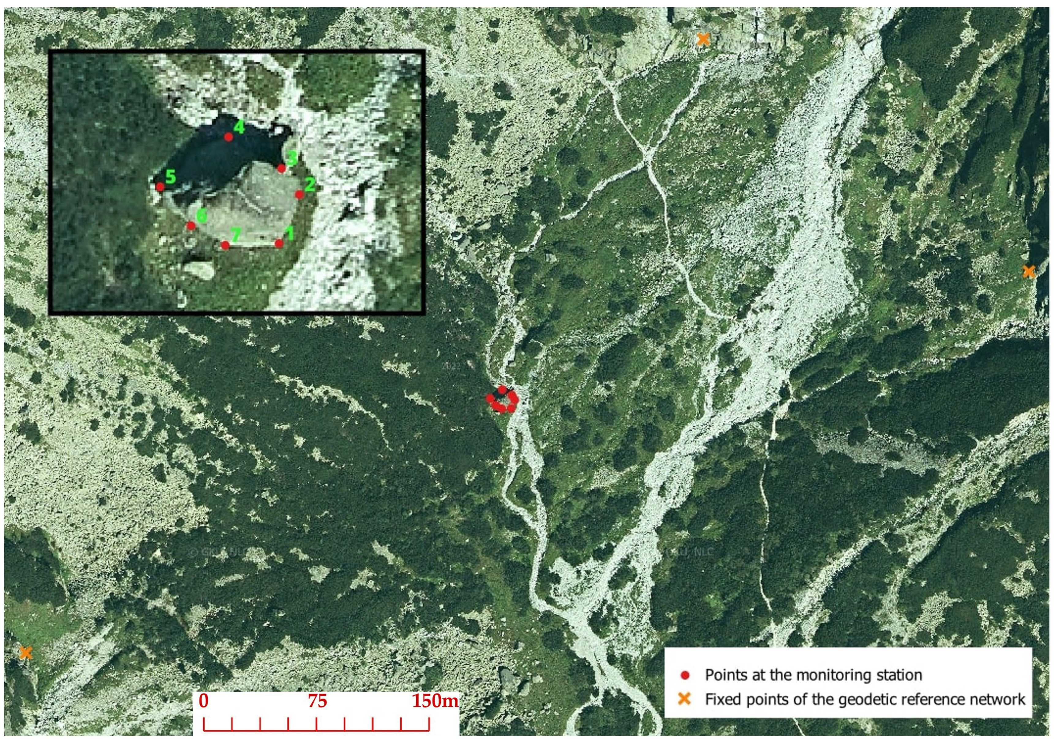
3.5. Establishment of a Monitoring Station

In 2022, a monitoring station was established on the massive boulder to monitor shifts and inclinations in three directions of its movement. On this boulder, 7 points were permanently stabilized by stainless steel pins. Stainless steel pins were drilled into the rock and fixed with Fischer chemical mortar. The location of the geodetic reference network points with 7 permanently stabilized points on the massive boulder is shown in Figure 10. The monitoring station was established on this boulder because its position is at the bottom of the Small Cold Valley in the bed of the Small Cold Stream. It is permanently washed by streams, especially in torrential rainfall events. We expect that the boulder can move in any direction in the future. Monitoring of shifts in the direction of the X, Y, and Z axes was realized using the following methods:

• Precise leveling.
• Spatial polar method with adjustment using Total Station.
• Terrestrial laser scanning.

The most accurate of these methods is precise leveling, where the expected height accuracy is up to 0.3 mm. Using the other two mentioned methods, we can determine the shifts at individual points in height and position, but these methods are less accurate. When measuring points by the spatial polar method, the expected accuracy in position is up to 1 mm and in height up to 2 mm and depends on the parameters of the total station and configuration of the surveying network. Using the TLS method, we can achieve an accuracy of 2–3 mm in position and up to 4 mm in height.

Precise leveling was carried out using a Leica DNA03 digital leveling instrument (Figure 11a) and two Leica invar code staffs. Selected technical parameters of the Leica DNA03 leveling device are listed in

Table 7. Technical specification of the leveling instrument Leica DNA03 [45].

Accuracy	±0.3 mm
Range	1.8–60 m
Resolution	0.01 mm
Magnification	24×
Compensator	Slope range: ± 10′ Setting accuracy: 0.3″
Measuring time	3 s
Internal memory	6000 measurements
Weight	2.8 kg
Operating temperature range	–20 °C to +50 °C

. During the leveling measurement, geometric leveling from the center and a closed leveling line with adjustment were used. It consists of 7 permanently stabilized points. The leveling line was measured twice, forth and back.

The second method in the first stage of measuring shifts at the monitoring station in the Small Cold Valley was the spatial polar method with adjustment. Measurement using this method was carried out by a Leica TS 06 total station (Figure 11b). A Leica GMP111 mini reflector prism was placed at each point of the monitoring station. The mini reflector prism was aimed from a free position of the total station on two faces of the telescope with three repetitions to increase the accuracy of the measurement.

The last method of monitoring shifts on the boulder was terrestrial laser scanning. A Leica RTC360 laser scanner was used for the TLS method (Figure 11c). This scanner is a mobile, automated, and efficient 3D laser scanner with a range of up to 130 m. Significant progress in this technology has been made using VIS technology to register the point cloud automatically in the field. VIS technology reduces the processing time and double scanning, thanks to which moving objects can be automatically removed. Selected technical parameters are shown in

Table 8. Technical parameters of laser scanner Leica RTC360 [46].

Type	High-speed, pulse, time-of-flight, Laser class 1
Weight	5.35 kg
Speed	Up to 2,000,000 points/s
Range	0.5 m–130 m
Accuracy	Distance: 1.0 mm + 10 ppm Angular: 18″
	3D points:	1.9 mm @ 10 m;
		2.9 mm @ 20 m;
		5.3 mm @ 40 m
Resolution	3 mm @ 10 m 6 mm @ 10 m 12 mm @ 10 m
Field of view	Horizontal: 360° Vertical: 300°
Operating temperature	−5 °C to +40 °C

. The measurement by the TLS method was carried out at eight positions for a little over one hour. At each station, at least three temporary black and white circular rotating scanning targets Leica GZT21 HDS 4.5 were scanned. They served as GCPs for the TLS method and were attached to permanently stabilized reference points of the monitoring station. The scanning resolution was set to medium, representing a value of 6 mm/10 m with a range of 130 m.

4. Data Processing

Data obtained using UAS photogrammetry were processed in Agisoft Metashape Professional software v. 1.8.0. Data obtained through terrestrial laser scanning were processed using Leica Cyclone software v. 9.2 (2018) and Leica Cyclone Register 360 software v. 2022.1 (epoch 2022). Trimble Realworks 10.0.4 software was used to prepare point clouds from UAS photogrammetry and TLS. Comparison and spatial analysis of point clouds was made using CloudCompare software v. 2.10.2.

4.1. Photogrammetric Processing

The first-stage (2018) photogrammetric images of the talus cone in the Small Cold Valley obtained using UAS were processed in the Agisoft Metashape Professional 1.5.0 software using the standard SfM workflow. A total of 1389 images were imported and aligned at high quality, resulting in a tie point. Due to the high level of detail and insufficient hardware performance in 2018, the entire talus cone area was divided into nine sub-blocks. A dense point cloud was individually generated with high-quality and mild-depth filtering. Subsequently, these nine point clouds were combined into one resulting point cloud, comprising 261,097,729 points. Other parameters of the resulting point cloud from 2018 obtained by the UAS photogrammetry method are shown in

Table 9. Parameters of point clouds from the first and second epoch.

	Point Cloud in Epoch 2018	Point Cloud in Epoch 2022
Number of images	1389	605
The number of tie points	337,415	286,306
The number of points of a dense point cloud	261,097,729	168,456,750
GSD [cm/pix]	0.95	1.50
Error in the X coordinate [mm]	5	13
Error in the Y coordinate [mm]	9	15
Error in the Z coordinate [mm]	4	9
RMSE on GCPs [mm]	11	36
RMSE on CPs [mm]	15	38

.

Using the UAS DJI Phantom 4 RTK, in the second measurement epoch of the talus cone in 2022, 605 images were captured. Photogrammetric data processing was carried out using Agisoft Metashape Professional 1.8.0 software. After importing the images and aligning them in high quality, 286,306 tie points were created. A dense point cloud with high-quality and mild-depth filtering was created in 5 h and 53 min and consisted of 168,456,750 points. In this case, dividing the area was unnecessary, and a dense point cloud was generated in one block. A closer specification of the dense point cloud from 2022 is described in Table 9.

4.2. TLS Data Processing

In 2018, in the first measurement epoch, the talus cone in the study area was scanned. Field data were processed using Leica Cyclone 9.2 software. Point clouds obtained from 25 positions were mutually registered and transformed into a unified coordinate system and georeferenced based on 16 GCPs. The resulting dense point cloud contained 597,031,328 points. The registration accuracy reached an average RMSE value of 0.001 m; at each station, the RMSE value was less than 0.003 m. After point cloud classification and vegetation removal, the point cloud contained 532,956,824 points. Despite the high number of points, the data obtained by the TLS method do not cover the entire terrain. It is a consequence of the terrain’s ruggedness and character, the scanner’s low position on the tripod and various obstacles during scanning.

In the second epoch in 2022, the Leica RTC360 laser scanner was used. Data were processed using Leica Cyclone Register 360 software. Point clouds from eight stations were imported into this software, registered, and georeferenced based on seven GPCs. The resulting dense point cloud consists of 445,171,906 points, reaching a total scan overlap of 38% and a strength of 75%. The bundle error value reached 0.006 m, and the Cloud-to-Cloud RMSE value was 0.009 m. The RMSE value on GCPs was determined to be 0.002 m.

4.3. ALS Data Processing

In the first epoch, data were also obtained from airborne laser scanning provided by The Geodesy, Cartography, and Cadastre Authority of the Slovak Republic (ÚGKK SR). They are divided to 42 areas (Figure 12) and available free of charge on a public web portal [47], where the full specification is provided. Data collection of area 26 was carried out in 2018 from June to September, and the selected territory extended into five flight strips. The parameters before the flight and the results obtained after the flight are available in

Table 10. Parameters of ALS in the epoch 2018.

Download date	12 February 2020
Version	Free
Format	Las 1.4 (classified point cloud), DTM, DSM
Coordinate system	Datum of Uniform Trigonometric Cadastral Network S-JTSK (implementation JTSK03); Baltic Vertical Datum—After Adjustment; ETRS89-h
Sensor	Riegl LMS-Q780
Flight height	3224 m ASL
Point density	before the classification	40 points/m2
	after the classification	14 points/m2
Overlap	40%
Point cloud	122,000 points

, where the resulting point cloud consists of 122,000 points. The point density value reaches an average of 15 cm, resulting in a thinner and less detailed point cloud.

5. Results

Concerning the final data obtained using UAS photogrammetry, TLS, and ALS, it was possible to perform analyses where point clouds were compared based on their mutual distance, detail, and accuracy. Before the actual comparison, the data were pre-processed, and we filtered unwanted and redundant points from each point cloud. Leica Cyclone 3DR v. 2020.0.6, Trimble Realworks ^® 10.0.4, and CloudCompare 2.10.2 software were used for processing, filtering, visualization, and comparison.

5.1. Comparison of Data from UAS Photogrammetry and TLS in 2018

In 2018, the talus cone was surveyed using two primary methods: UAS photogrammetry and TLS. After the processing of data sets, analysis of the resulting point clouds was carried out. Each point cloud was trimmed to the boundary of the study area of 4400 m². It guarantees the same compared area for both sets. The mean overall RMSE in UAS photogrammetry reached values of 11 mm and 1.2 mm for TLS. The area of the talus cone (Figure 13) was analyzed based on the comparison of height difference with the setting of the scale range to 75 mm, 150 mm, and 600 mm. With the scale range set to 75 mm, the Leica Cyclone 3DR software showed that most points (91%) ranged from 37.5 mm to −37.5 mm. In this case, there was a systematic shift in the entire range by −6 mm. If the scale range was set to 150 mm, the total systematic shift increased by 1 mm from the previous comparison. The largest representation of points was in the scale range from 75 mm to −75 mm, which represented 97% of the points. The last set range of the scale up to 600 mm presents 98% of the points located in the interval from 150 mm to −150 mm, while also, in this analysis, there was a shift. Several aspects had a negative impact on the standard deviation in the entire area, which reached an average value of 20 mm.

To confirm the systematic shift and standard deviation, spatial analyses were also carried out on smaller partial areas without vegetation. The first partial location (Figure 14a) was an area of 66 m², which was formed only by rocks of various sizes. This part was captured by 205,699 points using UAS photogrammetry and 86,771 points using the TLS method. The scale range was set to 150 mm, where the systematic shift of −6 mm was confirmed. As a result, 87% of the points were in the scale range from 56.2 mm to −37.5 mm. The second partial area (Figure 14b) for verification and comparison was a boulder whose total area was 6 m². The boulder was documented by 22,766 points by UAS photogrammetry and 19,180 points by the TLS method. Places that could not be sufficiently captured are marked in gray and are not included in the comparison. For this part, the scale range was set to 25 mm. The average standard deviation for all parts was 20 mm, which verified the cloud of points obtained by UAS photogrammetry.

5.2. Comparison of Data from UAS Photogrammetry and ALS in 2018

In this case, the point clouds from the 2018 epoch, obtained by UAS photogrammetry and ALS, were compared. Both involve acquiring data from different flying carriers and sensors. For UAS photogrammetry, the flight height AGL was set to approximately 35 m. ALS data were captured from an altitude of 3224 m ASL, which represents a difference of 1500 m in height. There is also the difference in the sensors used; a smaller unmanned aerial vehicle was used for UAS photogrammetry, and a larger piloted aircraft was used for ALS. A comparison can be made based on the number of points in the resulting point clouds. In UAS photogrammetry, the resulting point cloud consists of more than 261,000,000 points with a total RMSE value of 11 mm. The resulting point cloud from ALS contains only 122,000 points with an average GSD of up to 15 cm. UAS photogrammetry dominates in smaller areas requiring detail and higher accuracy. We compared both methods in the area of the talus cone, which had a size of 4400 m². The point clouds from both methods were trimmed to reduce the number of points and to unify the range of the compared area. For UAS photogrammetry, the final point cloud consisted of more than 14,000,000 points; for ALS, it consisted of more than 82,000 points. We compared the entire selected area based on the height difference (Figure 15), where the scale range was set to 10 mm, 50 mm, 100 mm, and 750 mm, respectively. When selecting the scale range of 10 mm, most points were located from −7.5 mm to −10 mm, representing 13.6%. When the scale range was set to 750 mm, most points were in the interval from 0 to −188 mm, where the percentual value was 54.5%.

Evaluation and comparison were also carried out at selected locations chosen because of their significance. The first such area was a location with an area of 1727 m² without vegetation. The chosen area contained 6,472,944 points, of which 6,441,540 were UAS photogrammetry points and 31,404 were points from ALS. Similarly, the scale range for this location was determined to be up to 10 mm, 50 mm, 100 mm, and 500 mm, respectively. It was clear from the analysis that most points were located at a difference of up to 100 mm (96%). Another analysis was performed on three almost equally sized areas (Figure 16a), which did not contain vegetation. These were located on the upper, middle, and lower parts of the talus cone. The largest had an area of 66 m², and the smallest had 42 m². Large rocks, various cracks, and gaps formed these places. For all surfaces, the scale range was determined from 150 mm to −150 mm, while the standard deviation of the height difference was 33 mm for all areas. The last comparison was made on three large rocks (Figure 16b), which were in the upper part of the entire site. For this study, the largest boulders with a slightly broken and evenly rounded surface located in the area of interest were chosen. Their area varied from 6 to 15 m². The limit range of the scale in this analysis was also set from 150 mm to −150 mm. The standard deviation of the height difference ranged from 19 to 26 mm. The density of points in UAS photogrammetry ranged from 7712 to 27,003 points, much more than ALS, where it was from 85 to 217 points.

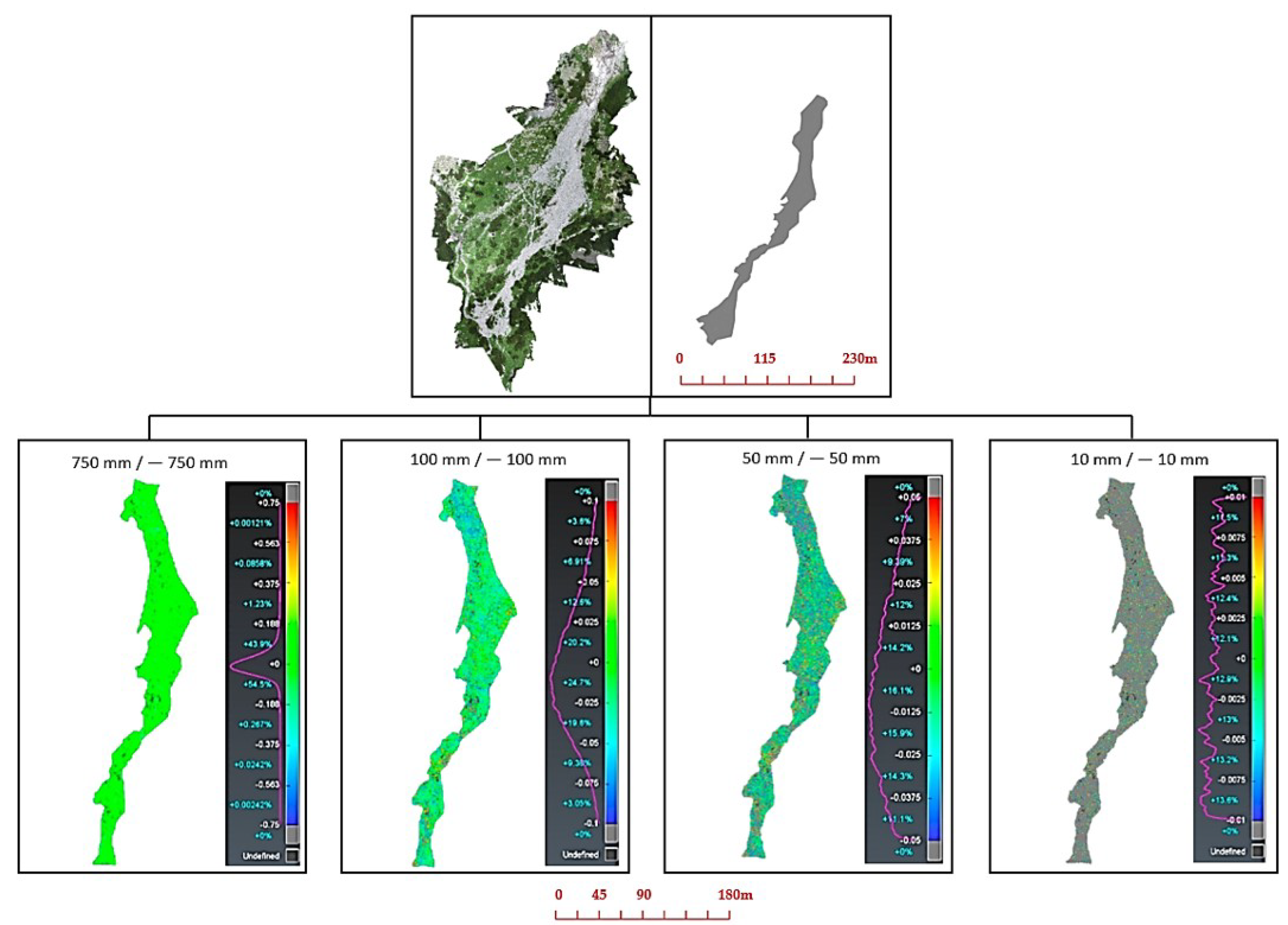
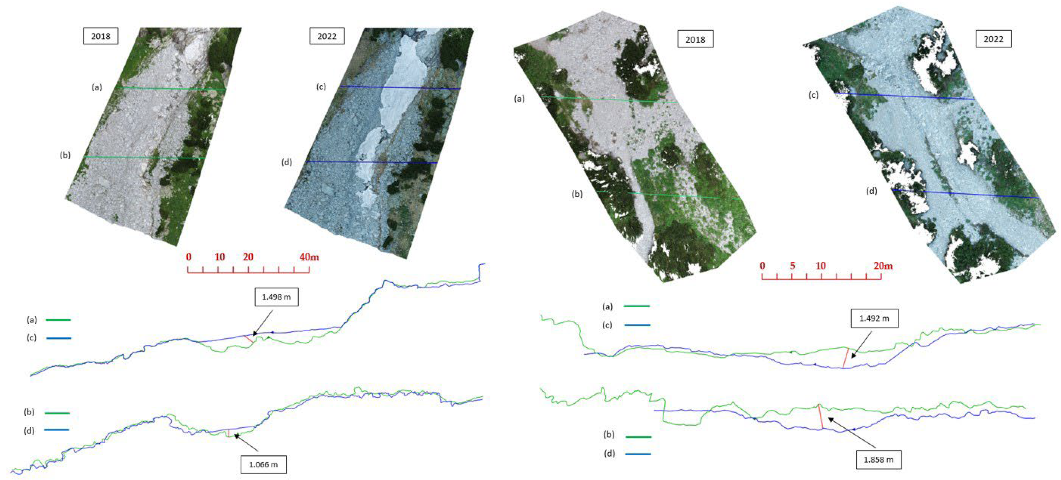
5.3. Comparison of Data from UAS Photogrammetry in Epochs 2018 and 2022

UAS data collection by photogrammetry was initially carried out in 2018 (Figure 17a) and 2022 (Figure 17c). The entire talus cone and its immediate surroundings were surveyed. Each point cloud was cropped, rasterized, and cleaned of vegetation, which reduced the number of points in epoch 2018 by 95% (Figure 17b) and in epoch 2022 by 91% (Figure 17d). When comparing point clouds, the most significant morphological changes occurred, according to Figure 17e, in the upper and lower parts. In the upper part of the study area, the change was caused by snow that had not yet melted. According to Figure 16e, snow thickness reached up to 2.5 m in some places. The most significant height difference also occurred in the area where natural factors created a deep bed in the stream flow. Over the years, flowing water has created a channel with rocks of different sizes. Due to the action of gravitational forces and the gradual release of the rock wall, they reach the lowest parts of the valley. There was a change in their positions, which was captured in the analysis with a height difference of up to 2.5 m.

It was also possible to document these significant changes with isolines and cross-sections (Figure 18), which show the changes caused in a selected part of the site in more detail and accuracy. Figure 18, left, shows the height difference located in the upper part of the monitored site. Two line segments were marked in each epoch. In the first epoch, they are line segments (a) and (b); in the second epoch, they are line segments (c) and (d), representing a cross-section of the terrain. Individual cross-sections are shown in the lower part of Figure 18, where the terrain from epoch 2018 is green, and the terrain from epoch 2022 is blue. During this comparison, the distance between the cross-sections was determined. A more significant change was noted when comparing cross-sections (a) and (c), the value of which was 1.498 m. This value does not represent the most significant distance in the compared section. The analysis in this form was also performed on the lower part of the talus cone (Figure 18 right), where the most significant changes occurred in the entire compared location. In this case, the cross-section distance was more considerable at segments (b) and (d), reaching a value of 1.858 m.

5.4. Monitoring Station: First Findings and Comparisons

First-stage (base) measurement at the monitoring station was carried out in June 2022 to monitor the displacements and shifts of seven permanently stabilized points on a massive stone block, i.e., a boulder. Monitoring the shifts in the direction of the X, Y, and Z axes were realized by precise leveling, spatial polar method, and terrestrial laser scanning. Second-stage measurement using the same methods was carried out in October 2022. We determined the height shift at the individual points of the monitoring station using the precise leveling method and the spatial polar method. The measured values in the first and second epochs are shown in

Table 11. Adjusted values of heights and differences between precise leveling and the spatial polar method.

Observed Point Nr.	Precise Leveling Z [m]		Difference [mm]	Spatial Polar Method Z [m]		Difference [mm]
	Base 1st Epoch	2nd Epoch		Base 1st Epoch	2nd Epoch
1	1640.00476	1640.00505	−0.3	1640.0083	1640.0082	0.1
2	1640.82483	1640.82670	−1.9	1640.8279	1640.8287	−0.8
3	1642.85170	1642.85457	−2.9	1642.8527	1642.8532	−0.5
4	1642.63407	1642.63164	2.4	1642.6328	1642.6331	−0.3
5	1642.98491	1642.98659	−1.7	1642.9896	1642.9886	1.0
6	1641.58462	1641.58395	0.7	1641.5875	1641.5882	−0.7
7	1640.36273	1640.36376	−1.0	1640.3617	1640.3625	−0.8

.

Only relative height differences were determined using the precise leveling method because connecting to any reference point with a given height was impossible. During processing, the heights were related to one observed point. The reason is the absence of reference points of the monitoring network near the measured object. Any reference points could not be stabilized since there was no solid rock in the available distance allowing its stabilization, i.e., the boulder was placed in sediment. Using the precise leveling method, the slightest deviation between the first and second epoch was 0.3 mm. The most significant deviation was found at point nr. 3 and reached 2.9 mm. With the spatial polar method, the smallest deviation in height was 0.1 mm, and the largest was 1.0 mm. The shifts in height between the first and second epoch at individual points measured by the precise leveling method are shown in Figure 19.

The spatial polar method with adjustment was considered the most suitable for determining horizontal shifts. The deviations between X and Y coordinates between epochs are shown in

Table 12. Horizontal coordinates in the first and second epochs and differences.

Observed Point Nr.	Base 1st Epoch		2nd Epoch		Differences
	X [m]	Y [m]	X [m]	Y [m]	X [mm]	Y [mm]
1	1,183,822.8861	336,967.2006	1,183,822.8870	336,967.1990	−0.9	1.6
2	1,183,818.2449	336,965.2630	1,183,818.2459	336,965.2617	−1.0	1.3
3	1,183,815.7554	336,966.9550	1,183,815.7564	336,966.9537	−1.0	1.3
4	1,183,812.7536	336,971.9885	1,183,812.7545	336,971.9871	−0.9	1.4
5	1,183,817.5043	336,978.4984	1,183,817.5053	336,978.4969	−1.0	1.5
6	1,183,821.2140	336,975.5514	1,183,821.2145	336,975.5502	−0.5	1.2
7	1,183,823.0606	336,972.3093	1,183,823.0621	336,972.3085	−1.5	0.8

. The most significant change in the X coordinate was determined at point nr. 7 and reached a value of −1.5 mm. The mean difference in the X coordinate between epochs reached a value of −0.94 mm. On the Y coordinate, the most significant shift was 1.6 mm at point nr. 1. The mean difference in the Y coordinate between epochs reached a value of +1.24 mm. Figure 20 shows spatial shift vectors at all points of the monitoring station. A black point represents the first epoch, the second epoch by an orange point, and the resulting shift is shown as a vector in purple. The X-axis is shown in green, the Y-axis in red, and the Z-axis in purple.

6. Discussion

The initial geodetic measurement in the location of the Small Cold Valley was carried out in June 2018. There, a talus cone created by rock debris from a landslide of a rock wall was documented as a priority. Continually, but mainly as a result of torrential rainfall with the melting of snow, rock massif was found to release huge rocks. Therefore, the first measurements were made to monitor the morphological changes to determine their size and dynamics. In our research [48], we carried out surveying works to establish and survey reference networks and perform base measurements by aerial photogrammetry and laser scanning. The measurements were carried out using up-to-date surveying instruments: UAS DJI Phantom 4 Pro, a Leica P40 laser scanner, GNSS set Leica GPS900cs, and Leica TS02 total station. The processed data provided sufficient results indicating the suitability and applicability of the selected measurement methods in the alpine environment. The spatial RMSE of UAS photogrammetry block adjustment evaluated on checkpoints reached a value of 0.011 m, while in TLS point cloud registration and georeferencing using GCPs, the RMSE value reached 0.001 m. Such accuracy is sufficient to monitor staged spatial morphology changes in the alpine environment. As a more suitable method to survey complex-shape terrain, we prefer aerial photogrammetry, which has its advantages in simplicity, complexity, speed, and low input costs. Therefore, photogrammetry opposes laser scanning, where the heavy instrument must constantly move over a complex surface. Other advantages and disadvantages of the used methods were stated by the authors in the article [48], where the financial costs of instrumentation and hardware equipment are also compared. In [49], the authors compared and evaluated the resulting point clouds from the first epoch. Analyses were performed on smaller partial areas (Figure 16) and the entire area of research. The high accuracy determined that the georeferenced point cloud obtained by the TLS method was designated as a reference. In 2020, airborne laser scanning (ALS) data at the study area, provided free of charge by the Geodesy, Cartography, and Cadastre Authority of the Slovak Republic (ÚGKK SR) through [47], were made available. ALS data were included in the comparison against other methods. A significant disadvantage of these data is the rarely updated sparse point cloud. From data obtained by UAS photogrammetry, TLS, and ALS methods, the RMSE of height differences in the entire compared area was determined to be 20 mm with a systematic shift of 6 mm [50]. When comparing point clouds from UAS photogrammetry and ALS, the average systematic shift had a value of 1 mm, with an RMSE value of 46 mm. After removing vegetation [51], the analysis was repeated, resulting in a change in the better RMSE value of 32 mm while the systematic shift value remained the same. The suitability of applying these methods can also be evaluated based on their density. The point cloud obtained by aerial photogrammetry represents 99.4% more points per m² than the ALS point cloud. Therefore, using UAS photogrammetry, observing small morphological changes in the terrain in more detail is possible. In [48], two point clouds obtained by UAS photogrammetry and TLS methods were compared based on distance, resulting in an RMSE value of 84 mm. After removing the vegetation, this RMSE value was determined to be 32 mm.

In June 2022, a second staged measurement was carried out in the location of the Small Cold Valley. Monitoring morphological changes was carried out using a more modern geodetic technique described by the authors in [52]. The research evaluates and compares the results from the first and second epochs. The final output point cloud accuracy in centimeter values was achieved. At the same time, detected changes represent differences in the range of meters (Figure 18). Significant changes were noted in the upper part of the talus cone, where there was still unmelted snow cover. Another significant morphological change was pointed out in the lower part, where there was a change in the river flow and bed due to the impact of rainfall events over the years. This process also caused a shift in the position of some rocks in the entire location. These changes are graphically shown in Figure 17 and Figure 18.

In June 2022, a monitoring station was also established in the research location to monitor spatial shifts and positional changes of separated stone blocks. Staged measurement allows the analysis of the shifts of seven points located on a massive stone block, i.e., a boulder, where we used the most accurate surveying instruments and methods. The achieved results are shown in Table 11 and Table 12. These tables also include deviations that indicate positional and height shifts. Height differences between stages are provided in (Figure 19). These data were determined using precision leveling (Figure 11a) and the spatial polar method with adjustment (Figure 11b). The application of the spatial polar method for the detection of spatial shifts is among the most suitable methods based on accuracy, speed, and simplicity. Despite the assumption of better results expected from precise leveling in the given environment and configuration of the measured points, the spatial polar method with adjustment appears more appropriate. This conclusion results from the RMSE values listed in Table 11. Worse values of precise leveling are also in the significant height differences between points at short distances. The reason is the necessity of inverse positioning of the leveling staff without the option of using any support stands. Another reason is the need to place the leveling instrument in the sediment or soft ground.

For interpreting the measurement of shifts and deformations, we considered the mean measurement error and the confidence coefficient, expressing the probability according to the chosen level of significance of the results. In practice, we considered the shift to be proven if its size exceeded two to three times the measurement accuracy. In our case, the displacement values reached just the level of measurement accuracy.

Using the TLS method, we documented the entire massive stone block with its surroundings. As a result, we created a 3D model, shown in the images in this chapter. So far, only one surveying stage has been carried out. Concerning the character of results and measurement accuracy of TLS, this method can be applied to survey shifts and deformations of boulders only when more significant movements are detected.

The surveying procedures and results of this study represent a properly proposed methodology for monitoring morphological changes. Of all techniques, UAS photogrammetry is the most effective and affordable method of mapping in the alpine environment, which can be applied to stage measurements in difficult-to-access terrain. This is also confirmed by research [53,54,55,56].

When assessing the TLS method, the advantage is that the result is a georeferenced point cloud with a high density. However, disadvantages include the high purchase cost of the equipment and the necessity for measurements from numerous scanning stations, which increases the time required for field measurements. UAS photogrammetry offers benefits such as speed of measurements in the field, the completeness of the final data, a dense point cloud with high density, and cost-effectiveness using UAS. The main disadvantage is that this method demands higher hardware requirements for image processing and longer data processing times. Due to freely available data, ALS measurements performed without direct field presence are perceived as the cheapest option. However, on the other hand, standard commercial ALS data are the most expensive dataset. The most problematic or expensive issue is also updating the data. Another disadvantage is also the lower density of the point cloud. The accuracy of terrain points obtained through ALS was comparable to the most precise terrestrial laser scanning method and UAS photogrammetry. This high accuracy results from the accuracy parameters of the device. TLS and UAS photogrammetry methods achieved a uniform density of several thousand points per m2. The ALS data had a much lower density. The use of the TLS method differed from the other two methods in terms of the difficulty of measurement due to the ruggedness of the terrain. With the UAS photogrammetry and ALS methods, the ruggedness of the terrain practically did not matter. A comparison of the methods used according to different parameters is presented in

Table 13. Comparison of the used methods according to different parameters.

	UAS Photogrammetry	TLS	ALS
Cost	Low cost	High purchase cost	High purchase and realization costs
Implementation	Flexible, quick, easy	Flexible, quick, difficult	Occasional campaign
Approximate shooting time	hours	days	days
Detail	High, full coverage	High, incomplete coverage	Low, incomplete coverage
Preferred research object	Small or mid-range areas	Small areas	Wide-range areas
Point density	High density	High density	Lower density
	3000 points/m2	3000 points/m2	40 points/m2

.

7. Conclusions

This article summarizes research and analysis of data obtained by various non-contact methods in difficult-to-access and rugged alpine terrain. The talus cone located in the Small Cold Valley in the High Tatras was documented as a priority. The monitoring of this talus cone was carried out in several stage measurements on different dates. Our research aimed to monitor and capture the morphological changes that occurred in some parts of the area. The obtained data were analyzed as point clouds cleaned of vegetation, trimmed, and reduced. During the first stage, based on the results of the analysis, it was possible to verify the suitability of the UAS photogrammetry method for monitoring changes in such locations. Due to the data’s detail, density, accuracy, and quality, this method is suitable for repeated data collection for monitoring changes. The main advantages of UAS photogrammetry are its low price, efficiency, high accuracy, and ease of use. In addition to the data obtained from the field by TLS and UAS photogrammetry, the authors also analyzed freely available data from airborne laser scanning, which was made available to the user in 2020. The results showed a systematic shift that ranged in centimeters. The standard deviation also achieved similar values, where values in the range of 0.03–0.05 m were reached. The significant difference between TLS and UAS photogrammetry data was in almost full area coverage by UAS photogrammetry against the TLS method, where TLS omits many joints and lowlands. The main reason was obstacles and rugged terrain, which made it impossible to reach hidden places with a laser scanner. We also found a difference in the density of points, which in UAS photogrammetry was uniform in the entire area with 3000 points per m². The density of ALS data in the study area was 17 points per m², indicating a lower point density. The TLS method was the most problematic of all the methods used. The reason was the high risk of damage to expensive equipment, high weight, incomplete coverage of the territory, and complicated movement between several positions. We verified the suitability of ALS for monitoring changes, even though this technology has lower accuracy and density than other methods. The presented research was devoted to comparing and evaluating the methods used in case studies, where certain results were achieved. Point clouds and their quality, density, detail, accuracy, and time required for the collection were analyzed. As a future study direction, this research will continue in consequent stages of surveying, even using newer non-contact mass data collection technologies. Data acquisition will be carried out directly in the field, from the air or from space. Further measurement is also planned at the monitoring station, where we monitor shifts in three directions on seven permanently stabilized points. The most suitable methods for monitoring shifts are precise leveling and the spatial polar method with adjustment, which are also planned to be used in further measurements.

References

1. Sepúlveda, S.A.; Alfaro, A.; Lara, M.; Carrasco, J.; Olea-Encina, P.; Rebolledo, S.; Garcés, M. An active large rock slide in the Andean paraglacial environment: The Yerba Loca landslide, central Chile. Landslides 2021, 18, 697–705. [Google Scholar] [CrossRef]
2. Marčiš, M.; Fraštia, M.; Hideghéty, A.; Paulík, P. Videogrammetric Verification of Accuracy of Wearable Sensors Used in Kiteboarding. Sensors 2021, 21, 8353. [Google Scholar] [CrossRef] [PubMed]
3. Tomek, L.; Beran, B.; Erdélyi, J.; Honti, R.; Mikula, K. Multichannel Segmentation of Planar Point Clouds Using Evolving Curves. Comput. Appl. Math. 2023, 42, 332. [Google Scholar] [CrossRef]
4. Salach, A.; Bakuła, K.; Pilarska, M.; Ostrowski, W.; Górski, K.; Kurczyński, Z. Accuracy Assessment of Point Clouds from LiDAR and Dense Image Matching Acquired Using the UAV Platform for DTM Creation. ISPRS Int. J. Geo-Inf. 2018, 7, 342. [Google Scholar] [CrossRef]
5. Kregar, K.; Marjetič, A.; Savšek, S. TLS-Detectable Plane Changes for Deformation Monitoring. Sensors 2022, 22, 4493. [Google Scholar] [CrossRef] [PubMed]
6. Szabó, S.; Enyedi, P.; Horváth, M.; Kovács, Z.; Burai, P.; Csoknyai, T.; Szabó, G. Automated registration of potential locations for solar energy production with Light Detection and Ranging (LiDAR) and small format photogrammetry. J. Clean. Prod. 2016, 112, 3820–3829. [Google Scholar] [CrossRef]
7. Hofierka, J.; Gallay, M.; Bandura, P.; Šašak, J. Identification of karst sinkholes in a forested karst landscape using airborne laser scanning data and water flow analysis. Geomorphology 2018, 308, 265–277. [Google Scholar] [CrossRef]
8. Fraštia, M.; Liščák, P.; Žilka, A.; Pauditš, P.; Bobáľ, P.; Hronček, S.; Sipina, S.; Ihring, P.; Marčiš, M. Mapping of Debris Flows by the Morphometric Analysis of DTM: A Case Study of the Vrátna Dolina Valley, Slovakia. Geogr. Časopis Geogr. J. 2019, 71, 101–120. [Google Scholar] [CrossRef]
9. Blistan, P.; Jacko, S.; Kovanič, Ľ.; Kondela, J.; Pukanská, K.; Bartoš, K. TLS and SfM Approach for Bulk Density Determination of Excavated Heterogeneous Raw Materials. Minerals 2020, 10, 174. [Google Scholar] [CrossRef]
10. Osińska-Skotak, K.; Bakuła, K.; Jełowicki, Ł.; Podkowa, A. Using Canopy Height Model Obtained with Dense Image Matching of Archival Photogrammetric Datasets in Area Analysis of Secondary Succession. Remote Sens. 2019, 11, 2182. [Google Scholar] [CrossRef]
11. Koska, B.; Křemen, T. The Combination of Laser Scanning and Structure from Motion Technology for Creation of Accurate Exterior and Interior Orthophotos of St. Nicholas Baroque Church. ISPRS Int. Arch. Photogramm. Remote Sens. Spat. Inf. Sci. 2013, 40, 133–138. [Google Scholar] [CrossRef]
12. Vanneschi, C.; Di Camillo, M.; Aiello, E.; Bonciani, F.; Salvini, R. SfM-MVS Photogrammetry for Rockfall Analysis and Hazard Assessment along the Ancient Roman via Flaminia Road at the Furlo Gorge (Italy). ISPRS Int. J. Geo-Inf. 2019, 8, 325. [Google Scholar] [CrossRef]
13. Gomez, C.; Setiawan, M.A.; Listyaningrum, N.; Wibowo, S.B.; Hadmoko, D.S.; Suryanto, W.; Darmawan, H.; Bradak, B.; Daikai, R.; Sunardi, S.; et al. LiDAR and UAV SfM-MVS of Merapi Volcanic Dome and Crater Rim Change from 2012 to 2014. Remote Sens. 2022, 14, 5193. [Google Scholar] [CrossRef]
14. Migliazza, M.; Carriero, M.T.; Lingua, A.; Pontoglio, E.; Scavia, C. Rock Mass Characterization by UAV and Close-Range Photogrammetry: A Multiscale Approach Applied along the Vallone dell’Elva Road (Italy). Geosciences 2021, 11, 436. [Google Scholar] [CrossRef]
15. Kovanič, L.; Blistan, P.; Rozložník, M.; Szabó, G. UAS RTK/PPK photogrammetry as a tool for mapping the urbanized landscape, creating thematic maps, situation plans and DEM. Acta Montan. Slovaca 2022, 26, 649–660. [Google Scholar] [CrossRef]
16. Kovanič, Ľ.; Blistan, P.; Štroner, M.; Urban, R.; Blistanova, M. Suitability of Aerial Photogrammetry for Dump Documentation and Volume Determination in Large Areas. Appl. Sci. 2021, 11, 6564. [Google Scholar] [CrossRef]
17. Wen, D.; Su, L.; Hu, Y.; Xiong, Z.; Liu, M.; Long, Y. Surveys of Large Waterfowl and Their Habitats Using an Unmanned Aerial Vehicle: A Case Study on the Siberian Crane. Drones 2021, 5, 102. [Google Scholar] [CrossRef]
18. Ajayi, O.G.; Ajulo, J. Investigating the Applicability of Unmanned Aerial Vehicles (UAV) Photogrammetry for the Estimation of the Volume of Stockpiles. Quaest. Geogr. 2021, 40, 25–38. [Google Scholar] [CrossRef]
19. Bakuła, K.; Pilarska, M.; Salach, A.; Kurczyński, Z. Detection of Levee Damage Based on UAS Data—Optical Imagery and LiDAR Point Clouds. ISPRS Int. J. Geo-Inf. 2020, 9, 248. [Google Scholar] [CrossRef]
20. Pavelka, K.; Matoušková, E.; Pavelka, K., Jr. Remarks on Geomatics Measurement Methods Focused on Forestry Inventory. Sensors 2023, 23, 7376. [Google Scholar] [CrossRef]
21. Kovanič, Ľ.; Topitzer, B.; Peťovský, P.; Blišťan, P.; Gergeľová, M.B.; Blišťanová, M. Review of Photogrammetric and Lidar Applications of UAV. Appl. Sci. 2023, 13, 6732. [Google Scholar] [CrossRef]
22. Braun, J.; Braunová, H.; Suk, T.; Michal, O.; Pěťovský, P.; Kurič, I. Structural and Geometrical Vegetation Filtering—Case Study on Mining Area Point Cloud Acquired by UAV Lidar. Acta Montan. Slovaca 2022, 26, 661–674. [Google Scholar]
23. Matoušková, E.; Pavelka, K.; Smolík, T.; Pavelka, K., Jr. Earthen Jewish Architecture of Southern Morocco: Documentation of Unfired Brick Synagogues and Mellahs in the Drâa-Tafilalet Region. Appl. Sci. 2021, 11, 1712. [Google Scholar] [CrossRef]
24. Available online: https://www.europeandataportal.eu (accessed on 22 August 2023).
25. Kyriou, A.; Nikolakopoulos, K.; Koukouvelas, I.; Lampropoulou, P. Repeated UAV Campaigns, GNSS Measurements, GIS, and Petrographic Analyses for Landslide Mapping and Monitoring. Minerals 2021, 11, 300. [Google Scholar] [CrossRef]
26. Guan, S.; Fukami, K.; Matsunaka, H.; Okami, M.; Tanaka, R.; Nakano, H.; Sakai, T.; Nakano, K.; Ohdan, H.; Takahashi, K. Assessing Correlation of High-Resolution NDVI with Fertilizer Application Level and Yield of Rice and Wheat Crops Using Small UAVs. Remote Sens. 2019, 11, 112. [Google Scholar] [CrossRef]
27. Štroner, M.; Urban, R.; Seidl, J.; Reindl, T.; Brouček, J. Photogrammetry Using UAV-Mounted GNSS RTK: Georeferencing Strategies without GCPs. Remote Sens. 2021, 13, 1336. [Google Scholar] [CrossRef]
28. Forlani, G.; Dall’Asta, E.; Diotri, F.; Cella, U.M.d.; Roncella, R.; Santise, M. Quality Assessment of DSMs Produced from UAV Flights Georeferenced with On-Board RTK Positioning. Remote Sens. 2018, 10, 311. [Google Scholar] [CrossRef]
29. Zeybek, M. Accuracy assessment of direct georeferencing UAV images with on-board global navigation satellite system and comparison of CORS/RTK surveying methods. Meas. Sci. Technol. 2021, 32, 065402. [Google Scholar] [CrossRef]
30. Braun, J.; Kremen, T.; Pruska, J. Micronetwork for Shift Determinations of the New Type Point Stabilization. In Proceedings of the 2018 Baltic Geodetic Congress (BGC Geomatics), Olsztyn, Poland, 21–23 June 2018; pp. 265–269. [Google Scholar] [CrossRef]
31. Pirti, A.; Hosbas, R.G. Evaluation of some levelling techniques in surveying application. Geod. Cartogr. 2019, 68, 361–373. [Google Scholar] [CrossRef]
32. Guevara Lima, J.R.; González Giraldo, S.M.; Sánchez Cárdenas, J.S. Methodological Proposal to Correct and Adjust a Geodesic Leveling Data. Tecciencia 2019, 14, 27. [Google Scholar] [CrossRef]
33. Santos, D.P.D.; Faggion, P.L.; Veiga, L.A.K. Camapuã Hill altitude determination from leap-frog trigonometric leveling method. Bol. De Ciências Geodésicas 2011, 17, 295–316. [Google Scholar] [CrossRef]
34. Lukniš, M. Reliéf Vysokých Tatier a Ich Predpolia; Vydavateľstvo SAV: Bratislava, Slovakia, 1973. [Google Scholar]
35. Bohuš, I. Od A po Z o názvoch Vysokých Tatier, 1st ed.; ŠL TANAPu: Tatranská Lomnica, Slovakia, 1996; ISBN 80-967522-7-8. [Google Scholar]
36. Radwańska-Parysky, Z.; Paryski, W.H. Wielka Encyklopedia Tatrzańska; Wydawnictwo Górskie: Poronin, Poland, 2004; ISBN 83-7104-009-1. [Google Scholar]
37. Fauna na území TANAP-u. Tatranský Národný Park. Available online: https://www.tanap.sk/priroda/fauna-3/ (accessed on 22 August 2023).
38. Černík, A.; Sekyra, J. Zeměpis Velehor; Academia: Prague, Czech Republic, 1969; 396p. [Google Scholar]
39. Midriak, R. Morfogenéza Povrchu Vysokých Pohorí; VEDA: Bratislava, Slovakia, 1983; 516p. [Google Scholar]
40. Available online: https://www.geotech.sk/downloads/Totalne-stanice/FlexLine_TS02_Datasheet_en.pdf (accessed on 24 November 2023).
41. Available online: https://www.geotech.sk/downloads/Totalne-stanice/FlexLine_TS06_Datasheet_en.pdf (accessed on 24 November 2023).
42. Available online: https://www.dji.com/sk/phantom-4-pro-v2/specs (accessed on 24 November 2023).
43. Available online: https://enterprise.dji.com/phantom-4-rtk/specs (accessed on 24 November 2023).
44. Available online: https://www.geotech.sk/downloads/Laserove-skenery-HDS/Leica%20ScanStation%20P30-P40%20FLY%200215_SK_PLANT2_fieldView.pdf (accessed on 24 November 2023).
45. Available online: https://www.geotech.sk/downloads/Nivelacne%20pristroje/Geodeticke/Nivelacny-pristroj-digitalny-DNA-prospekt_EN.pdf (accessed on 24 November 2023).
46. Available online: https://www.geotech.sk/downloads/Laserove-skenery-HDS/Leica_RTC360_sk2.pdf (accessed on 24 November 2023).
47. Available online: https://www.geoportal.sk/sk/zbgis/lls/ (accessed on 27 November 2023).
48. Urban, R.; Štroner, M.; Blistan, P.; Kovanič, Ľ.; Patera, M.; Jacko, S.; Ďuriška, I.; Kelemen, M.; Szabo, S. The Suitability of UAS for Mass Movement Monitoring Caused by Torrential Rainfall—A Study on the Talus Cones in the Alpine Terrain in High Tatras, Slovakia. ISPRS Int. J. Geo-Inf. 2019, 8, 317. [Google Scholar] [CrossRef]
49. Kovanič, Ľ.; Blistan, P.; Urban, R.; Štroner, M.; Blišťanová, M.; Bartoš, K.; Pukanská, K. Analysis of the Suitability of High-Resolution DEM Obtained Using ALS and UAS (SfM) for the Identification of Changes and Monitoring the Development of Selected Geohazards in the Alpine Environment—A Case Study in High Tatras, Slovakia. Remote Sens. 2020, 12, 3901. [Google Scholar] [CrossRef]
50. Štroner, M.; Urban, R.; Línková, L. Multidirectional Shift Rasterization (MDSR) Algorithm for Effective Identification of Ground in Dense Point Clouds. Remote Sens. 2022, 14, 4916. [Google Scholar] [CrossRef]
51. Štroner, M.; Urban, R.; Suk, T. Filtering Green Vegetation Out from Colored Point Clouds of Rocky Terrains Based on Various Vegetation Indices: Comparison of Simple Statistical Methods, Support Vector Machine, and Neural Network. Remote Sens. 2023, 15, 3254. [Google Scholar] [CrossRef]
52. Kovanič, Ľ.; Štroner, M.; Urban, R.; Blišťan, P. Methodology and Results of Staged UAS Photogrammetric Rockslide Monitoring in the Alpine Terrain in High Tatras, Slovakia, after the Hydrological Event in 2022. Land 2023, 12, 977. [Google Scholar] [CrossRef]
53. Szypuła, B. Accuracy of UAV-Based DEMs without Ground Control Points. GeoInformatica 2023, 28, 1–28. [Google Scholar] [CrossRef]
54. Štroner, M.; Urban, R.; Křemen, T.; Braun, J. UAV DTM Acquisition in a Forested Area—Comparison of Low-Cost Photogrammetry (DJI Zenmuse P1) and LiDAR Solutions (DJI Zenmuse L1). Eur. J. Remote Sens. 2023, 56. [Google Scholar] [CrossRef]
55. Šašak, J.; Gallay, M.; Kaňuk, J.; Hofierka, J.; Minár, J. Combined Use of Terrestrial Laser Scanning and UAV Photogrammetry in Mapping Alpine Terrain. Remote Sens. 2019, 11, 2154. [Google Scholar] [CrossRef]
56. Vazquez-Tarrío, D.; Borgniet, L.; Li´ebault, F.; Recking, A. Using UAS optical imagery and SfM photogrammetry to characterize the surface grain size of gravel bars in a braided river (V’en’eon River, French Alps). Geomorphology 2017, 285, 94–105. [Google Scholar] [CrossRef]
Figure 1. Location of the study area in Small Cold Valley, High Tatras.
Land 13 00112 g001
Figure 2. Optimized procedure for performing geodetic works.
Land 13 00112 g002
Figure 3. Stabilization of the points of the precise geodetic network (a) stainless steel pins, (b) reflective foils.
Land 13 00112 g003
Figure 4. Position of stabilized points of the precise geodetic network in 2018 (a) and 2022 (b).
Land 13 00112 g004
Figure 5. Position, numbering and signalization (details in blue boxes) of GCP for photogrammetry in 2018 (a) and 2022 (b).
Land 13 00112 g005
Figure 6. Total station Leica TS02 (a) and GNSS set Leica GS07 (b).
Land 13 00112 g006
Figure 7. Position and numbering of GCPs for TLS method in 2018.
Land 13 00112 g007
Figure 8. UAS DJI Phantom 4 Pro (a) and DJI Phantom 4 RTK (b).
Land 13 00112 g008
Figure 9. Three-dimensional terrestrial laser scanner Leica ScanStation P40.
Land 13 00112 g009
Figure 10. Position and numbering of stabilized points of the geodetic reference network and points at the monitoring station.
Land 13 00112 g010
Figure 11. Instruments used for surveying in the monitoring station. Leveling instrument Leica DNA03 (a), total station Leica TS06 (b), and laser scanner Leica RTC360 (c).
Land 13 00112 g011
Figure 12. ALS area nr. 26 with the resulting point cloud.
Land 13 00112 g012
Figure 13. Comparison of point clouds: UAS photogrammetry and TLS method according to the selected scale range.
Land 13 00112 g013
Figure 14. Analyzing two smaller partial areas without vegetation: (a) smaller area and (b) boulder.
Land 13 00112 g014
Figure 15. Comparison of point clouds: UAS photogrammetry and ALS according to the selected scale ranges up to 750 mm, up to 100 mm, up to 50 mm, up to 10 mm.
Land 13 00112 g015
Figure 16. Analysis and comparison smaller areas: UAS photogrammetry and ALS according to the selected scale ranges; (a) smaller rock field, (b) single boulders.
Land 13 00112 g016
Figure 17. Comparison of UAS photogrammetry point clouds from epochs 2018 and 2022; raw point cloud (a) epoch 2018, (c) epoch 2022; filtered point cloud (b) epoch 2018, (d) epoch 2022.
Land 13 00112 g017
Figure 18. Cross-sections on smaller areas with the most significant difference.
Land 13 00112 g018
Figure 19. Shifts in height between the first and second epoch on observed points obtained by the precise leveling method (up—position and numbering of points, left—south view, right—north view).
Land 13 00112 g019
Figure 20. Shifts in three directions (X, Y, Z) at all points of the monitoring station (top view); red dots displays position with green numbering of points.
Land 13 00112 g020