Accounting for and Comparison of Greenhouse Gas (GHG) Emissions between Crop and Livestock Sectors in China

Abstract

The synergistic greenhouse gas (GHG) emission reduction of the crop production (CP) and livestock farming (LF) sectors is of great significance for food security and low-carbon development, especially for China, the world leader in agricultural production. In this paper, the GHG emissions from the CP and LF sectors are accounted for and compared, and the spatial econometric model is adopted for comparative study based on the panel data from 1997 to 2021. The results show that: (1) The total amount and intensity of GHG emissions from both sectors showed obvious spatial heterogeneity and spatial dependence, and the spatial distribution pattern was relatively stable. (2) The influence of each factor on the GHG intensity and spatial characteristics of CP and LF varies widely. For the CP sector, economic development (local effect −0.29, adjacent effect +1.13), increased urbanization rate (−0.24, +0.16), agricultural structure (−0.29, +0.05), and urban-rural disparity (−0.03, +0.17) all reduce the GHG intensity of local region, while increasing the GHG intensity of its adjacent areas, signifying leakage. The economic structure (+0.06, +0.16), agricultural finance support (+0.02, +0.26), mechanization level (+0.05, +0.03), and land occupancy rate (+0.54, +0.44) all play a role in increasing the GHG intensity of CP in the local region and its adjacent areas. The disaster degree (−0.03, −0.03) also reduced the GHG intensity of CP. For the LF sector, economic structure (+0.08, +0.11), urban-rural disparity (+0.11, +0.21), agricultural development level (+0.03, +0.50), and increased land occupancy rate (+0.05, +0.01) can improve the GHG intensity of the one region and adjacent areas. Economic development (+0.03, −0.15), urbanization rate (+0.04, −0.30), agricultural structure (+0.09, −0.03), and disaster degree (+0.02, −0.06) can increase the GHG intensity of the local region while reducing the GHG intensity of adjacent areas. Based on the results, under the background of carbon peaking and carbon neutralization(dual-carbon) goals, this study first puts forward collaborative emission reduction measures for CP and LF, respectively, then further rises to sector synergy and regional synergy, and constructs the countermeasure system framework of collaborative emission reduction from three levels, to provide guidance and reference for the realization of dual goals of agricultural GHG reduction and food security.

1. Introduction

The rapid development of agriculture is inevitably accompanied by the deterioration of the environment and the emergence of a series of ecological problems, especially greenhouse gas (GHG) emissions. This issue has been widely concerning due to the increasing climate change [1]. Agriculture has become one of the major emitters of GHG, producing about 14% of global GHG emissions and 58% of global non-carbon (CH₄, N₂O) GHG emissions [2,3]. Moreover, if effective measures are not taken as soon as possible, the agricultural GHG is expected to increase by 30% by 2050 [4], making it hard to realize the emissions reduction target of the Paris Agreement. As a world leader in agriculture production, China feeds 20% of the world’s population with only 8% of global cropland [5,6]. Since the launch of the reform and opening up policy, China has made remarkable and rapid achievements in agriculture; the output of grain, meat, and aquatic products in 2017 has reached 1/5, 1/4, and 1/3 of world supplies after a 2-fold, 10-fold, and 14-fold increase since 1978, respectively [7]. However, great achievements in agriculture have come at the cost of large amounts of GHG emissions. China’s agricultural GHG have accounted for 17% of the national emissions [8], of which agricultural CH₄ and N₂O emissions are much higher than other industries; agricultural CH₄ emissions accounted for 50.15% of the total emissions, and N₂O accounted for 92.43% of total emissions [9,10].

Unlike other sectors, agriculture is more dependent on region-specific factors, such as topography, soil, and climate [11], as well as on socioeconomic factors, including mechanization, irrigation, and the supply-demand situation of agricultural products. Therefore, the differences among region-specific factors have led to heterogeneity in agriculture, which may have caused spatial variations in agricultural GHG emissions. China has a vast territory and a wide distribution of agriculture. Due to significant differences in agricultural production conditions and resource endowments among provinces, there are large disparities in the agricultural development level and its structure. Extensive research has been conducted on these regional disparities using various indicators, such as total agricultural GHG emissions [12,13,14], agricultural GHG intensity [15,16], net agricultural GHG [17], and agricultural GHG efficiency(productivity) [16,18,19]. These indicators all show obvious regional heterogeneity in agricultural GHG emissions. However, most of the related studies used the concept of “agriculture” to account for GHG emissions, treating crop production (CP) and livestock farming (LF) as one whole subject. A small number of studies separately examine GHG emissions from LF and find significant spatial significance in both the total amount and intensity of GHG emissions. When it comes to the factors influencing GHG, researchers have found that the level of economic development [20,21], urbanization [20], technological development [22], agricultural economic level [23], agricultural structure [20,24], level of agricultural mechanization [22], agricultural human resources [25], and agricultural disaster severity [20] are the main factors influencing agricultural GHG emissions and their spatial heterogeneity. Additionally, there is a certain degree of spatial spillover effect, meaning that the agricultural GHG emissions of one province are not independent but are influenced by its surrounding provinces [23,26,27].

Although there have been studies on the spatial heterogeneity of agricultural or livestock GHG emissions, the majority of these studies included LF GHG emissions in agriculture. However, the distribution of the CP and LF sectors varies across provinces in China, resulting in spatial distribution heterogeneity for CP and LF GHG emissions. Treating them as a whole in research would hide or weaken the spatial heterogeneity at a more micro level. It would also mask the specific mechanisms of certain influencing factors, leading to a significant discount in the targeted formulation of GHG reduction policies. Moreover, the CP and LF sectors have strong complementarity, as CP provides feed for LF, and LF provides organic fertilizers for CP sector. The synergetic action between the two can theoretically achieve win-win benefits and GHG emissions reduction. Furthermore, there is currently limited literature on the spatial spillover effects of agricultural GHG emissions, and the existing studies mainly focus on the existence of spillover effects, paying less attention to the magnitude and direction of these effects.

Therefore, this research aims to fill the gap by following aspects. First of all, the paper innovatively divides agriculture into CP and LF, investigates the spatial distribution of GHG emissions for each sector, respectively, and explores the mechanisms of their respective interactions with relevant factors. Then, the spatial heterogeneity and influencing mechanisms of certain factors can be presented more specifically at a more micro level. Secondly, the research further examines spatial spillover mechanisms of both sectors. The spillover effect of agricultural GHG among provinces is widespread [23,26,27], while limited studies have explored it in depth. Last but not least, a strategic system for coordinated emission reduction in both sectors is designed based on the empirical results, which is a breakthrough in the research of agricultural GHGs. In the context of China’s dual-carbon goals, this study has both theoretical value and practical significance.

The rest of this paper is organized as follows (Figure 1). In Section 2, we present the accounting process of GHG emissions from CP and LF and the theoretical aspects of the spatial Durbin model (SDM). In Section 3, the spatial variation of GHG emissions from CP and LF is firstly demonstrated from the scale and intensity, followed by the results and discussion of SDM results. Synergic measures were put forward in Section 4, and we concluded in Section 5.

2. Materials and Methods

2.1. GHG Accounting

The agricultural GHG accounting system based on the life cycle assessment (LCA) method has been well-developed. The current system mainly includes the CO₂, N₂O, and CH₄ emissions generated throughout the entire production process, including soil emissions, energy input, and material input [28,29,30] (

Table 1. GHG accounting process and data sources.

GHG Types	GHG Sources	Accounting Process and Data Sources
GHG from crop production	a. N2O from crop cultivation	The planting area of different crops such as rice, wheat (spring and winter wheat), soybean, maize, vegetables, sorghum, millet, potato, and peanut are multiplied by their respective N2O emission coefficients and then converted into the CO2 equivalent. The planting area of various crops comes from the China Statistical Yearbook and the China Agricultural Yearbook.
	b. Indirect emissions from agricultural inputs	The quantity of different inputs such as chemical fertilizer, diesel, pesticide, agricultural film, machinery power, and irrigation area is multiplied by the emission coefficients to obtain the quantity of CO2 emission. The data on various types of agricultural inputs come from the China Agricultural Yearbook and New China Agriculture 60 Years Statistics.
	c. CH4 emissions from paddies	CH4 emissions from early, late, and mid-season rice (single-cropping late rice, winter paddy field, and wheat stubble rice) in different provinces were obtained by multiplying the planting areas with respective emission coefficients and then converted into CO2 equivalent. The area data of various types of paddy fields come from the China Agricultural Yearbook.
GHG from livestock farming	d. CH4 and NO2 from ruminant activities and manure management	After converting the sales quantity and stock quantity of pigs, cattle, sheep, horses, donkeys, and mules into the annual average feeding quantity, the CH4 and N2O emissions obtained by multiplying the annual average feeding quantity of different animals with the emission coefficients are converted into CO2 equivalent. Data on the number of animals sold out and the number of animals in stock are from the China Agricultural Yearbook.

). Specifically, the agricultural GHG encompasses four main parts: a. N₂O emissions from crop production. This mainly refers to N₂O emissions during soil tillage, and the emission coefficients (

Table A1. Coefficients for N₂O from crop cultivation.

Sources	Emission Coefficients (kg·hm−2)
Rice	0.24
Spring-season wheat	0.4
Winter-season wheat	1.75
Soybean	2.29
Maize	2.532
Vegetables	4.944
Other dryland crops	0.95

) per unit area of different crops vary [20]. b. Indirect emissions from agricultural inputs: This mainly includes the indirect GHG generated by the use of pesticides, plastic films, electricity, fertilizers, diesel, and other agricultural inputs during the production process (

Table A2. Coefficients for indirect emissions from agricultural inputs.

GHG Sources	Emission Coefficients
Pesticide	4.9341 kg·kg−1
Chemical fertilizer	0.8956 kg·kg−1
Agricultural film	5.18 kg·kg−1
Agricultural irrigation	266.48 kg·hm−2
Agricultural machinery	0.18 kg·kW−1
Agricultural energy(diesel)	0.5927 kg·kg−1

). c. CH₄ emissions from paddy fields. This refers to the direct CH₄ emissions generated by paddy fields. The emission coefficients (

Table A3. Coefficients for CH₄ emissions from paddies.

Provinces	Early-Season Rice	Mid-Season Rice	Late-Season Rice
Beijing	0	13.23	0
Tianjin	0	11.34	0
Hebei	0	15.33	0
Shanxi	0	6.62	0
Inner Mongolia	0	8.93	0
Liaoning	0	9.24	0
Jilin	0	5.57	0
Heilongjiang	0	8.31	0
Shanghai	12.41	53.87	27.5
Jiangsu	16.07	53.55	27.6
Zhejiang	14.37	57.96	34.5
Anhui	16.75	51.24	27.6
Fujian	7.74	43.47	52.6
Jiangxi	15.47	65.42	45.8
Shandong	0	21	0
Henan	0	17.85	0
Hubei	17.51	58.17	39
Hunan	14.71	56.28	34.1
Guangdong	15.05	57.02	51.6
Guangxi	12.41	47.78	49.1
Hainan	13.43	52.29	49.4
Chongqing	6.55	25.73	18.5
Sichuan	6.55	25.73	18.5
Guizhou	5.1	22.05	21
Yunnan	2.38	7.25	7.6
Tibet	0	6.83	0
Shaanxi	0	12.51	0
Gansu	0	6.83	0
Qinghai	0	0	0
Ningxia	0	7.35	0
Xinjiang	0	10.5	0

) per unit area vary due to the hydrological, climatic, and soil conditions of different provinces, as well as the rice planting season (early-, middle-, or late-season rice) [1]. d. GHG emissions from livestock. This includes the CH₄ and N₂O emissions generated by manure management and ruminant activities of herbivorous animals (

Table A4. Coefficients for GHGs from ruminant activities and manure management.

Sources	CH4 from Ruminant Activities (kg per Year)	CH4 from Manure Management (kg per Year)	NO2 from Manure Management (kg per Year)
Non-dairy cattle	51.4	1.5	1.37
Dairy cattle	68	16	1
Horses	18	1.64	1.39
Donkeys	10	0.9	1.39
Mules	10	0.9	1.39
Pigs	1	3.5	0.53
Sheep	5	0.16	0.33

). The sum of emissions from a, b, and c represents the GHG emissions from crop cultivation, while d represents the emissions from livestock breeding. The accounted N₂O and CH₄ emissions are converted into CO₂ equivalents using the conversion factors for greenhouse gases provided by the IPCC. The CO₂ equivalent values are divided by the output value of crop cultivation and livestock breeding, respectively, to obtain the GHG intensities of crop cultivation and livestock breeding for each province in different years.

2.2. Model Setting

Given the spatial correlation and spatial heterogeneity of GHG emission intensities in CP and LF, this study adopts a spatial econometric model to explore the spatial heterogeneity effects and its influencing factors. To validate the rational selection of the model, the spatial autocorrelation of GHG intensities in both sectors needs to be tested before entering the spatial econometric model. Spatial autocorrelation can be divided into global autocorrelation and local autocorrelation [31], which respectively investigate whether there is a spatial correlation among all spatial units as a whole and the specific form of correlation between individual spatial units and their surrounding units. In this study, only the global spatial autocorrelation of CP and LF GHG intensity is verified to demonstrate the scientific and rational application of the spatial econometric model. The commonly used indicator for testing global autocorrelation is Moran’s I, and the formula for calculation is as follows [21,32]:

$$Moran\text{’}sI=\frac{n{\sum }_{i=1}^n{\sum }_{j\ne 1}^n{W}_{ij}(x_i-\overline{x})(x_j-\overline{x})}{{\sum }_{i=1}^n(x_i-\overline{x}){\sum }_{i=1}^n{\sum }_{j=1}^n{W}_{ij}}$$

(1)

where $n$ represents each province, $x_i$ represents the GHG intensity of province i, $\overline{x}$ represents the average GHG intensity of all provinces and $W_{ij}$ represents the spatial matrix between provinces i and j. Considering the model test results and the province-level agricultural situation, after systematic comparison and reference to similar literature, this study uses a simple and classical binary adjacency matrix, where two regions with a common boundary are considered adjacent [31,33]. The values on the main diagonal are set to 0, and W_ij for adjacent provinces is set to 1; otherwise, it is set to 0 (Hainan is considered adjacent to Guangdong). Moran’s I ranges between −1 and 1, where a value greater than 0 indicates positive spatial correlation and clustering of GHG intensity among provinces, a value less than 0 indicates discrete distribution, and Moran’s I = 0 indicates random distribution. The larger the absolute value of Moran’s I, the greater the spatial correlation of GHG intensity among provinces.

Spatial econometric models effectively address the limitations of traditional regression models that assume spatial homogeneity, making them more reliable when applied to research subjects involving spatial autocorrelation [31]. Spatial econometric models can be divided into the spatial error model (SEM), spatial lag model (SLM), and SDM [33]. Among them, the SEM focuses on analyzing the differences in the form of interactions between different regions, and the SLM is commonly used to study the spillover effects of variables on regions outside the focal region. The SDM can be seen as a synthesis of the SLM and the SEM, which can be simplified to a SEM or a SLM under certain conditions [33]. The theoretical form of the SDM is as follows:

$$Y_t=\delta \ast W\ast Y_t+{{\beta }_1\ast X}_t+{\beta }_2{\ast W\ast X}_t+v_t$$

(2)

In the Equation (2), $Y_t$ represents a 31 × 1 vector of GHG intensity in each province at time t (number of provinces), $X_t$ represents a 31 × K matrix of exogenous explanatory variables, where K is the number of selected explanatory variables, W represents a 31 × 31 spatial weight matrix, which is also based on geographical adjacency, $W\ast X_t$ represents the interaction term between the spatial weight matrix and the exogenous explanatory variables, and $\delta ,\beta$ represents the corresponding coefficients to be estimated. If ${\beta }_2$ is zero, the SDM can be simplified to a SLM, and if ${\beta }_2+\delta \ast {\beta }_1=0$, the SDM can be simplified to a SEM. The theoretical form of the SDM, further simplified by removing the subscript t, is as follows:

$$Y=({I-\delta W)}^{-1}\ast ({\beta }_{1}W+{\beta }_{2}WX)+{(I-\delta W)}^{-1}$$

(3)

Taking the partial derivative of Y with respect to the k-th explanatory variable of the i-th province yields:

$$\left[\frac{\partial Y}{\partial x_{1k}}\cdots \frac{\partial Y}{\partial x_{Nk}}\right]=\left[\begin{array}{ccc}\frac{\partial y_1}{\partial x_{1k}}& \cdots & \frac{\partial y_1}{\partial x_{Nk}}\\ ⋮& \ddots & ⋮\\ \frac{\partial y_N}{\partial x_{1k}}& \cdots & \frac{\partial y_N}{\partial x_{Nk}}\end{array}\right]={(I_N-\delta W)}^{-1}\left[\begin{array}{cccc}{\beta }_{1k}& w_{12}{\beta }_{2k}& \cdots & w_{1N}{\beta }_{2k}\\ w_{21}{\beta }_{2k}& {\beta }_{1k}& \cdots & w_{2N}{\beta }_{2k}\\ ⋮& ⋮& \ddots & ⋮\\ w_{N1}{\beta }_{2k}& w_{N2}{\beta }_{2k}& \cdots & {\beta }_{1k}\end{array}\right]={\left(I-\delta W\right)}^{-1}({\beta }_{1k}{I}_N+{\beta }_{2k}W)$$

(4)

The direct effects of the SDM represent the average change in the dependent variable (GHG emission intensity) in a province caused by the explanatory variable of that province, which is the average of the diagonal elements of Equation (4) ($\overline{d}$ denotes the average of the diagonal elements of the matrix):

$$\mathrm{direct} \mathrm{effects}={\left[{(I_N-\delta W)}^{-1}({\beta }_{1k}{I}_N+{\beta }_{2k}W)\right]}^{\overline{d}}$$

(5)

The indirect effects of the SDM refer to the average change in the dependent variable (GHG emission intensity) in neighboring provinces caused by the explanatory variable of a province, which is the average of the off-diagonal elements of Equation (4) ($\overline{rsum}$ denotes the average of the off-diagonal elements of the matrix):

$$\mathrm{indirect} \mathrm{effects}={\left[{(I_N-\delta W)}^{-1}({\beta }_{1k}{I}_N+{\beta }_{2k}W)\right]}^{\overline{rsum}}$$

(6)

The total effect is the sum of the direct effects and indirect effects [33]. As for whether the SDM in this study can be simplified to a SEM or a SLM, as well as the choice of fixed effects or random effects models, they can be determined through the Wald test, LR test, and Hausman test to select the most suitable model form. The model testing and empirical analysis in this study were conducted using the Stata 15.0.

2.3. Variable Definition

In this study, the dependent variables are the GHG intensity of the CP and LF sectors. When selecting the independent variables, we try to choose variables that could potentially affect both the CP and LF sectors in order to compare the different mechanisms of the same variable on the GHG intensity of both sectors. Based on relevant studies on the factors influencing agricultural production and GHG emissions [34,35,36,37,38,39,40], two categories of 10 indicators are chosen as explanatory variables (

Table 2. Model variables.

Variable Type	Variable Name	Description	Max	Min.	Mean	SD
Independent variable	CP GHG intensity	GHG emissions/crop production value	0.3827	0.0172	0.0966	0.453
	LF GHG intensity	GHG emissions/livestock production value	1.9294	0.0080	0.2045	2.952
Explanatory variable	Economic development level	Per capita GDP	33.04	2.21	8.26	0.546
	Economic structure	Proportion of added value of primary industry	37.840	0.360	13.426	7.448
	Urbanization rate	Urban population/total population	0.896	0.149	0.481	0.163
	Urban-rural disparity	Urban/rural consumption level	8.900	1.500	3.036	0.829
	Agricultural structure	Output value of crop production/output value of livestock farming	5.224	0.803	2.124	0.775
	Agricultural financial support	The proportion of financial support for agriculture in total financial expenditure	0.190	0.021	0.092	0.033
	Disaster degree	Disaster-affected area/crop planting area	0.936	0.000	0.257	0.163
	Agriculture development level	Agricultural added value/rural population	1.354	0.133	0.510	0.268
	Mechanization level	Agricultural machinery power/rural population	10.845	0.026	1.196	0.810
	Land occupancy rate	Arable land area/rural population	10.301	0.634	2.228	1.678

). The first category represents the macro development of each province, including economic development level, economic structure, urbanization rate, and urban-rural disparity, totaling four indicators. The second category represents the agricultural development situation of each province, including agricultural structure, agricultural financial support, disaster degree, agricultural development level, mechanization level, and arable land occupancy rate, totaling six specific indicators. It is worth noting that in the process of calculating these indicators, data such as output value and value-added have been adjusted to constant prices in 1997. For some provinces and years, rural population data were missing, and the annual changes were minimal. Therefore, the moving average method was used to fill in the missing data. Before entering the empirical model, all indicators were standardized. Furthermore, before the regression analysis, we first tested the multicollinearity. The variance inflation factor (VIF) index of all the selected variables was less than 10, indicating that there was no significant collinearity between them. The meanings and descriptive statistics of each indicator are shown in Table 2.

3. Results

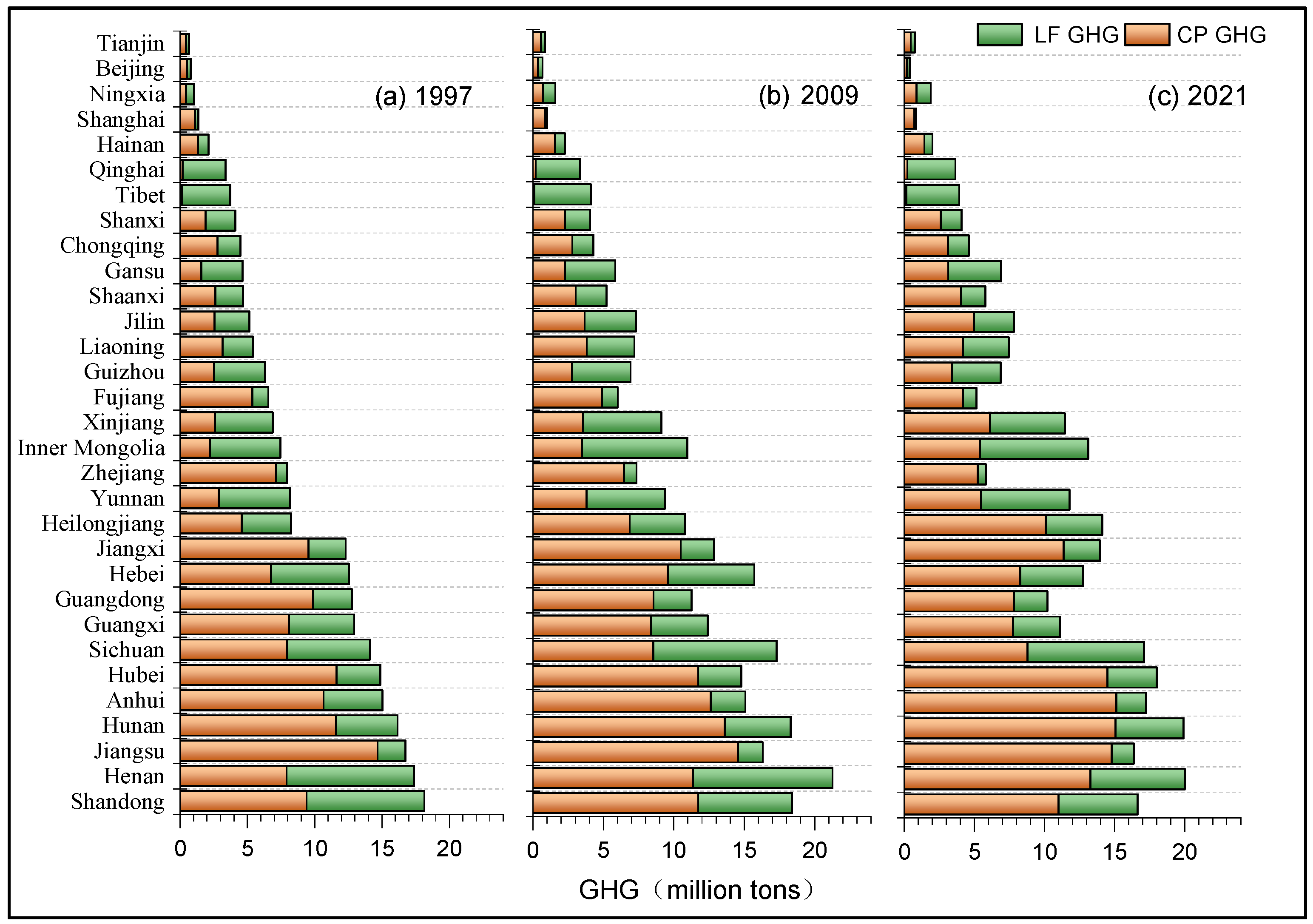
3.1. Spatial Distribution of GHG Emissions for CP and LF Sectors

In terms of the national total, the agricultural GHG emissions in 1997, 2009, and 2021 reached 256.24 million tons, 282.74 million tons, and 293.19 million tons, respectively (Figure 2). The total agricultural carbon emissions show an increasing trend at the beginning, but the growth rate has slowed down sharply and is even showing signs of a peak point. Actually, some studies have shown a peak in China’s agricultural GHG emissions in recent years [21,41]. Comparing the GHG emissions from the CP and LF sectors of each province (Figure 2), it can be seen that provinces with a strong tradition of agriculture have higher total GHG emissions, and in most provinces, GHG emissions from the CP sector are higher than those from the LF sector. Provinces in the northwest such as Qinghai, Tibet, Ningxia, and Inner Mongolia, which are mainly focused on the LF sector, have relatively low total GHG emissions, but the GHG emissions from the LF sector are significantly higher than those from the CP sector. Yunnan, Sichuan, and other provinces also have slightly higher GHG emissions from the LF sector compared to the CP sector. The comparison of the CP and LF GHG emissions reflects the spatial pattern of CP and LF production in each province. Furthermore, the total agricultural GHG emissions and the proportion of GHG emissions from the CP and LF sectors have remained relatively stable over the years, indicating that the structure of the CP and LF industries in each province is relatively stable.

Individually, looking at the GHG intensity of the CP sector (Figure 3), traditional grain-producing provinces such as Hubei, Hunan, Jiangxi, and Guangxi generally have higher GHG intensity. Among the above provinces, southern ones have higher GHG intensity than those in the northern part. This is mainly because of the higher proportion of rice in the crop structure of southern provinces. The GHG footprint of rice in China is 3.3 times that of maize and 2.1 times that of wheat [20]. In terms of GHG intensity in the LF sector, provinces such as Tibet, Qinghai, Inner Mongolia, and Xinjiang are significantly higher than other provinces, and they also have higher GHG emissions from livestock compared to provinces with high livestock GHG emissions, such as Henan and Sichuan. This is because these provinces have a higher proportion of ruminant animals, such as cattle and sheep, in their LF sector, and these animals have much higher GHG intensity due to the CH₄ emissions from rumination.

Comparing the carbon intensity of the CP and LF sectors, it can be seen that the GHG intensity in the LF sector is much higher than that in the CP sector in all provinces, further confirming the viewpoint that the GHG footprint of livestock is higher than that of crop production [42]. Looking at the trends over the years (Figure 3), the GHG intensity of CP and LF sectors in each province has decreased significantly, owing to the substantial improvement in agricultural production efficiency in China in recent years [5]. However, the distribution pattern of GHG intensity in the CP and LF sectors remains relatively stable. The LF GHG intensity is still high in provinces such as Qinghai, Tibet, Ningxia, and Inner Mongolia, which focus on LF, while the CP GHG intensity in provinces such as Hunan and Jiangxi has also been consistently higher than that in other provinces.

3.2. Spatial Autocorrelation Test

A spatial autocorrelation test on the GHG emission intensity of the CP and LF sectors is conducted to explore whether provinces with similar GHG emission intensity show spatial clustering and some degree of spatial heterogeneity.

During the entire study period, the p-values and z-values of Moran’s I for LF GHG intensity passed the test, and Moran’s I for every year were greater than 0, indicating significant spatial autocorrelation and strong spatial clustering of LF GHG intensity. For CP GHG intensity, most years also showed spatial autocorrelation, but a few years (2012–2017) did not pass the test (Figure 4). Nevertheless, this still suggests the presence of spatial autocorrelation and spatial clustering in the CP GHG intensity. The main reason is that the calculated Moran’s I is based on a simple binary geographic adjacency matrix, which assumes that if spatial units are not adjacent, they do not influence each other, and even if they are adjacent, it assumes equal influence, which cannot fully explain the spatial clustering of GHG intensity. For example, in 2017, Sichuan Province had a crop-to-livestock output ratio of 2.4, while the ratios of Chongqing and Guizhou in the eastern neighborhood were 1.9 and 3.2, respectively, and the ratios of Qinghai and Tibet in the western neighborhood are only 1.1 and 1.6.

The spatial autocorrelation is relatively stable in the historical trends, especially for Moran’s I of LF GHG emission intensity. The Moran’s I of LF GHG intensity shows a downward trend over time (Figure 4), which indicates that in the context of significantly improved overall agricultural production efficiency in China [5], the provinces that originally had high GHG emission intensity experienced a gradual decrease in production efficiency improvement. The gap between them and provinces with low emission intensity is gradually narrowing. It should be noted that Moran’s I aims to prove the existence of spatial spillover effect and is only the first step to verifying the rationality of SDM [43,44,45]. The following steps, such as the Hausmann test, LM test, and LR test, will be conducted to show the existence of spatial effect and prove the suitability of spatial econometric models.

3.3. Model Test

A Lagrange multiplier (LM) test was conducted to further examine the suitability of the spatial econometric models. According to the criteria proposed by Anselin (1991) and the LM test results (

Table 3. LM test statistics and significance.

LM Test		CP Sector	LF Sector
Spatial error model	Lagrange multiplier	213.494 ***	257.791 ***
	Robust Lagrange multiplier	128.813 ***	14.577 ***
Spatial lag model	Lagrange multiplier	85.530 ***	321.804 ***
	Robust Lagrange multiplier	0.849	78.590 ***

Note: *** p < 0.01.

), it is found that the CP GHG intensity is better suited for a SEM, while the LF GHG intensity is better suited for a SDM. Subsequently, the Hausman test results (

Table 4. Hausmann test results.

Variable Classification	Statistic	p-Value
CP GHG intensity	10.59	0.5646
LF GHG intensity	486.05	0.0000

) indicate that the CP GHG intensity should use a fixed effects model, while the LF sector is better suited for a random effects model. It can be seen from the likelihood ratio (LR) test that both the time fixed effects and individual fixed effects are significant. Therefore, the appropriate model for the CP sector is the time-individual fixed effects model. The Wald test and LR test results (

Table 5. Results of Wald test and LR test.

Test Types	Variables	Can SDM Be Simplified to SAR?	Can SDM Be Simplified to SEM?
LR test	CP GHG intensity	41.70 ***	40.07 ***
	LF GHG intensity	86.61 ***	157.55 ***
Wald test	CP GHG intensity	33.26 ***	40.88 ***
	LF GHG intensity	87.90 ***	150.10 ***

Note: *** p < 0.01.

) reject the hypothesis that the SDM can degenerate into the SEM and the spatial autoregressive model at a 1% significance. To summarize, the CP GHG emission intensity is best analyzed using an individual-time fixed effects spatial Durbin model, while the LF sector is more suitable for a random effects spatial Durbin model.

3.4. Results of SDM

The regression results of the SDM (

Table 6. SDM estimation results.

Explanatory Variables	CP GHG Intensity		LF GHG Intensity
	Main Effects (Main)	Spatial Effects (Wx)	Main Effects (Main)	Spatial Effects (Wx)
Economic development level	−0.315 *** (0.113)	1.053 *** (0.304)	0.0422 (0.0504)	−0.101 (0.107)
Economic structure	0.0638 (0.0544)	0.117 (0.135)	0.0767 *** (0.0242)	0.0285 (0.0361)
Urbanization rate	−0.244 *** (0.0552)	0.169 (0.124)	0.0545 ** (0.0264)	−0.202 *** (0.0560)
Urban-rural disparity	−0.0360 ** (0.0297)	0.158 ** (0.0685)	0.0915 *** (0.0137)	0.0808 *** (0.0230)
Agricultural structure	−0.296 *** (0.0436)	0.0719 (0.0871)	0.0859 *** (0.0196)	−0.0516 (0.0323)
Agricultural financial support	0.0141 (0.0400)	0.234 *** (0.0898)	−0.0728 *** (0.0182)	−0.158 *** (0.0272)
Disaster degree	−0.0255 ** (0.0189)	−0.0260 ** (0.0382)	0.0214 ** (0.00939)	−0.0426 ** (0.0179)
Agriculture development level	−0.636 *** (0.0643)	−0.148 ** (0.141)	−0.00245 (0.0294)	0.294 *** (0.0519)
Mechanization level	0.0464 ** (0.0235)	0.0210 (0.0504)	−0.0346 *** (0.0114)	−0.0148 (0.0216)
Land occupancy rate	0.533 *** (0.0814)	0.345 * (0.181)	0.0530 ** (0.0360)	−0.0165 (0.0678)
Constant			0.00997 (0.146)
ρ	0.113 * (0.0594)		0.440 *** (0.0458)
R2	0.6158		0.6578
Log-likelihood	−927.1855		−927.1855

Note: *** p < 0.01, ** p < 0.05, * p < 0.1; Values in parentheses are the standard deviations.

) show that the autoregressive coefficients of the CP and LF emission intensity pass the test at the 10% and 1% confidence levels, respectively.

From the regression coefficients and their significance, it can be observed that for the CP sector, factors such as economic development level, urbanization level, agricultural structure, and agricultural development level can locally reduce GHG intensity. In particular, the inhibitory effect of agricultural development level is the most significant. On the other hand, the mechanization level and land occupancy rate increase CP GHG emission intensity, with the latter having a larger impact. In terms of spatial effects, factors such as economic development level, rural-urban disparity, agricultural financial support, and land occupancy rate can increase the GHG intensity of neighboring areas, with economic development level having the most significant influence.

For the LF sector, the mechanization level and financial support for agriculture play a certain inhibitory role in the region, although their effects are relatively weak. On the other hand, economic structure, urbanization rate, rural-urban disparity, agricultural structure, and disaster degree contribute to increased LF GHG emissions. Rural-urban disparity and agricultural development level can promote GHG intensity in neighboring provinces, while urbanization rate, agricultural financial support, and disaster degree can inhibit GHG intensity in adjacent areas.

After determining whether various factors have an impact on the GHG intensity of the CP and LF sectors in the local and neighboring areas, the direct effects, indirect effects, and total effects of these factors are discussed to distinguish the effects of each factor more accurately (Figure 5). It can be observed that there are significant differences in the effects of various factors on the GHG intensity of the CP and LF sectors, whether in the local or adjacent areas. Although the regression coefficients of some factors’ direct effects or indirect effects are not significant, the magnitude and direction of these effects on the GHG intensity of the CP and LF sectors can still be observed to some extent.

Firstly, for the CP sector, factors such as economic development level (direct effect −0.29; indirect effect +1.13), urbanization level (−0.24; +0.16), rural-urban disparity (−0.03; +0.17), and agricultural structure (−0.29; +0.05) can reduce the GHG intensity in the local area while increasing the GHG intensity in neighboring areas, with the increasing effect of economic development level being particularly significant. Economic structure (+0.06; +0.16), agricultural financial support (+0.02; +0.26), mechanization level (+0.05; +0.03), and land occupancy rate (+0.54; +0.44) can increase the GHG intensity of the CP sector in both the local and adjacent areas, while the disaster degree (−0.03; −0.03) can reduce the GHG intensity in both areas.

For the LF sector, factors such as economic structure (+0.08; +0.11), rural-urban disparity (+0.11; +0.21), agricultural development level (+0.03; +0.50), and land occupancy rate (+0.05; +0.01) can increase the GHG intensity in both the local and adjacent areas, although the increasing effect of land occupancy rate is small. Economic development level (+0.03; −0.15), urbanization level (+0.04; −0.30), agricultural structure (+0.09; −0.03), and disaster degree (+0.02; −0.06) have an increasing effect on GHG intensity in the local area but reduce the GHG intensity in adjacent areas, with urbanization level having the most significant effect on reducing the LF GHG intensity in adjacent areas. Both agricultural financial support (−0.10; −0.31) and mechanization level (−0.04; −0.05) factors can reduce the carbon emission intensity of the livestock sector in both the local and adjacent areas, but the regression coefficient former factor is much larger than that of mechanization level.

In summary, the mechanisms of various factors on the GHG intensity of the CP and LF sectors are significantly different. In terms of the magnitude of their effects on both sectors, factors such as economic development level, agricultural development level, and land occupancy rate have a greater impact on the GHG intensity of the CP sector while having a smaller impact on the GHG intensity of the LF sector. In terms of the direction of their effects on both sectors, factors such as economic development level, urbanization level, agricultural structure, agricultural financial support, agricultural development level, and mechanization level show completely opposite effects, i.e., while increasing the GHG intensity of the CP sector, they can reduce the GHG intensity of the LF sector, and vice versa. It is generally believed that an increase in per capita arable land will improve production efficiency due to the scale effect of agricultural production, thereby reducing agricultural GHG emissions. However, this study found that per capita arable land has a certain increasing effect on the GHG intensity of the CP sector after separating the CP and LF sectors. This may be because provinces with a higher per capita arable land are mainly grain-producing areas, such as the northeast provinces, compared to other provinces producing cash crops, which have relatively lower value-added products, resulting in relatively higher GHG intensity (GHG emissions per unit of value-added).

4. Construction of a Synergistic GHG Reduction System

As agriculture plays a fundamental role in food supply, emission reduction measures in the CP and LF sectors should ensure a coordinated and comprehensive approach. It is necessary to guarantee food security while reducing GHG emissions in the production process, contributing to the achievement of the carbon reduction goals. In the context of dual-carbon goals, based on the differences in spatial distribution and influencing mechanisms of the CP and LF sectors, this study first proposes specific emission reduction measures tailored to each sector. Then, based on the synergy of multiple measures, it further progresses to the coordination of crop–livestock integration and regional coordination, proposing a strategic framework for coordinated emission reduction at three levels (Figure 6). This framework aims to provide guidance and reference for achieving dual goals of agricultural GHG reduction and food security.

4.1. Synergistic Measures

Because of the significant differences in the spatial distribution and influencing mechanisms of the CP and LF sectors, specific emission reduction measures need to be formulated for each sector. For the CP sector, while ensuring food supply, measures such as improving nitrogen fertilizer efficiency, optimizing irrigation patterns, developing nitrification inhibitors, and exploring new nitrogen fertilizer technologies can reduce emissions of N₂O from fertilizer sources [46]. Measures such as precise fertilizer regulation, optimizing cultivation practices, implementing organic matter return, and optimal water management can help reduce CH₄ emissions from paddy fields. Implementing plans to reduce inputs and increase the efficiency of agrochemicals such as fertilizers, pesticides, and agricultural films can indirectly achieve GHG reduction by improving agricultural eco-efficiency and reducing input quantities. In addition to emissions reduction, the carbon sequestration capacity of soil should not be overlooked. By promoting the development of technologies related to soil organic carbon, emission reduction, and carbon sequestration can be achieved in coordination. For the LF sector, the main sources of GHG emissions are enteric fermentation and manure management. Measures such as precision feeding, rapid CH₄ monitoring, and optimizing feeding structures can be implemented to reduce CH₄ emissions from enteric fermentation. Regarding manure management, measures such as manure return to fields, biogas utilization, and inhibition of GHG synthesis can be adopted to reduce emissions. Furthermore, promoting standardized and ecological farming practices and optimizing the structure of LF can be effective means of reducing GHG emissions.

4.2. Crop-Livestock Integration

Continued efforts should be made to promote the transformation of agricultural production towards a circular “resources—products—renewable resources—products” mode and accelerate the development of integrated crop-livestock circular agriculture. This approach will achieve overall economic, ecological, and social benefits greater than the sum of its parts. Promoting the recycling of crop straws is an important step. Establishing a sound system for straw collection, storage, and transportation, promoting the utilization of straw as feed, and popularizing technologies such as straw silage, baling, ammonization, and pellet production can serve as a linkage for driving integrated crop-livestock systems. Additionally, the utilization of livestock manure for biogas production, through the construction of biogas digesters, can tightly connect the livestock and crop sectors, achieving the integrated development of crop-livestock systems and biogas industries. This can effectively reduce agricultural GHG emissions and achieve energy substitution for energy savings and emission reductions in other sectors.

4.3. Regional Coordination

Given the spatial heterogeneity of the CP and LF sectors and their different mechanisms of factors, regional synergy in agricultural GHG reduction should be implemented from three aspects: (a) Measures need to be tailored to local conditions. Considering varying economic, social, and agricultural conditions, each province or region should formulate GHG reduction policies in the CP and LF sectors that are tailored to their specific circumstances. For example, agricultural financial support policies can increase CP GHG emissions intensity for both local provinces and neighboring provinces, but for the LF sector, it can significantly reduce GHG intensity in the local provinces and surrounding provinces. Therefore, using agricultural financial support policies to achieve GHG emissions reduction goals is only applicable to major livestock-producing provinces, while traditional major CP provinces may need to rely on other measures. (b) Regional collaboration is crucial. Both the CP and LF sectors have evident spatial spillover effects on GHG intensity. One single factor that reduces local GHG intensity may also affect or even increase GHG intensity in neighboring areas. This “domino effect” necessitates increased cooperation among provinces when formulating relevant GHG reduction measures. Joint exploration of GHG reduction technologies and improved agricultural resource utilization efficiency should be pursued. (c) Top-down coordination is necessary. At the national level, a unified strategy should be employed, considering overall grain supply and food security. This involves coordinating and optimizing the production layout of the CP and LF sectors.

5. Conclusions

Broadly defined, GHG emissions in agriculture include both the CP and LF sectors. However, studying them as a whole may obscure or weaken the micro-level spatial characteristics and specific mechanisms of factors. This study separates the CP and LF sectors from the macro “agriculture” and conducts separate research on their GHG emissions characteristics. Spatial econometric models are used to explore and compare the spatial characteristics and mechanisms of factors of both sectors. A system of coordinated measures, integrated crop-livestock production, and regional collaboration for emissions reduction is then proposed. The main conclusions and policy implications are as follows.

The spatial distribution of GHG emissions in the CP and LF sectors is consistent with the spatial patterns in each province. Because the GHG emission intensity of LF is much higher than that of the CP sector, and the GHG intensity of rice planting is higher than that of other planting, the GHG emission intensity of all provinces shows obvious spatial heterogeneity. The growth rate of total agricultural GHG has slowed down sharply and is even showing signs of an inflection point in recent years due to the significant drop in intensity for both sectors caused by the increase in agricultural productivity. At a critical time when agricultural GHG is approaching the peak point and with the need for carbon neutrality, further improvement in agricultural productivity is necessary. However, agriculture is a prerequisite for human survival and development, and the GHG reduction in this field must be made only if food supplies are met.

The magnitude of the impact of different factors on GHG intensity in the CP and LF sectors also varies dramatically. Traditionally, the increase of agricultural financial support and mechanization level are all important policy tools to boost agricultural productivity. However, our more specific empirical research showed that the increase in agricultural financial support and mechanization level can increase the GHG intensity of the CP sector while decreasing the GHG intensity in the LF sector. Other factors also affect both CP and LF sectors at different magnitudes and directions, indicating that agricultural GHG reduction policies need to be tailored to specific sectors. The spatial spillover effects of both sectors also have important policy implications. When formulating a certain policy tool to reduce local GHG emissions, its increasing effect on the GHG of neighboring areas must be considered comprehensively, which requires the coordination of higher-level authorities. Provinces with higher CP GHG intensity are often the main food-supplying regions that play a strategic role in the whole country or even worldwide, so when considering GHG reduction, their contribution to food security should be emphasized.

This study has certain inadequacies, which require further research in the future. Although a more detailed study than previous research was conducted, the classification of the sectors still needs to be more specific. Research on specific crop species or animal types is necessary. Furthermore, our investigation focuses on a provincial perspective. In the future, the following research should deepen the research to a more microscopic level. The research at the county level is of greater significance to the micro-level GHG emission mechanism and GHG reduction policies.

References

1. Qu, J.S.; Han, J.Y.; Liu, L.N.; Xu, L.; Li, H.J.; Fan, Y.J. Inter-provincial correlations of agricultural GHG emissions in China based on social network analysis methods. China Agric. Econ. Rev. 2020, 13, 229–246. [Google Scholar] [CrossRef]
2. IPCC. Climate Change 2007: Mitigation of Climate Change. Contribution of Working GroupⅢ to the Fourth Assessment Report of the Intergovernmental Panel on Climate Change; Cambridge University Press: Cambridge, UK, 2007. [Google Scholar]
3. Beach, R.H.; Deangelo, B.J.; Rose, S.; Li, C.; Salas, W.; DelGrosso, S.J. Mitigation potential and costs for global agricultural greenhouse gas emissions. Agric. Econ. 2008, 38, 109–115. [Google Scholar] [CrossRef]
4. Tubiello, F.N.; Salvatore, M.; Golec, R.D.C.; Ferrara, A.; Rossi, S.; Biancalani, R.; Federici, S.; Jacobs, H.; Flammini, A. Agriculture, forestry and other land use emissions by sources and removals by sinks: 1990–2011 analysis. In FAO Statistics Division; FAO: Rome, Italy, 2014; Volume 4, pp. 375–376. [Google Scholar]
5. Zeng, J.J.; Han, J.Y.; Qu, J.S.; Maraseni, T.N.; Xu, L.; Li, H.J.; Liu, L.N. Ecoefficiency of China’s agricultural sector: What are the spatiotemporal characteristics and how are they determined? J. Clean. Prod. 2021, 325, 129346. [Google Scholar] [CrossRef]
6. Zhang, L.; Pang, J.X.; Chen, X.P.; Lu, Z.M.N. Carbon emissions, energy consumption and economic growth: Evidence from the agricultural sector of China’s main grain-producing areas. Sci. Total Environ. 2019, 665, 1017–1025. [Google Scholar] [CrossRef] [PubMed]
7. Liu, Y.S.; Zou, L.L.; Wang, Y.S. Spatial-temporal characteristics and influencing factors of agricultural eco-efficiency in China in recent 40 years. Land Use Policy 2020, 97, 104794. [Google Scholar] [CrossRef]
8. He, Y.Q.; Cheng, X.Y.; Wang, F.; Cheng, Y. Spatial correlation of China’s agricultural greenhouse gas emissions: A technology spillover perspective. Nat. Hazards 2020, 104, 2561–2590. [Google Scholar] [CrossRef]
9. Han, M.; Zhang, B.; Zhang, Y.; Guan, C.H. Agricultural CH4 and N2O emissions of major economies: Consumption-vs. production-based perspectives. J. Clean. Prod. 2019, 210, 276–286. [Google Scholar] [CrossRef]
10. Zhang, H.Y.; Xu, Y.; Lahr, M. The greenhouse gas footprints of China’s food production and consumption (1987–2017). J. Environ. Manag. 2021, 301, 113934. [Google Scholar] [CrossRef]
11. Lepadatu, C. Effects of market reform on agricultural policy community and rural areas. Sci. Pap. 2012, 12, 39–42. [Google Scholar]
12. Cui, Y.; Khan, S.U.; Deng, Y.; Zhao, M. Regional difference decomposition and its spatiotemporal dynamic evolution of Chinese agricultural carbon emission: Considering carbon sink effect. Environ. Sci. Pollut. Res. 2021, 28, 38909–38928. [Google Scholar] [CrossRef]
13. Xu, X.C.; Zhang, N.; Zhao, D.X.; Liu, C.J. The effect of trade openness on the relationship between agricultural technology inputs and carbon emissions: Evidence from a panel threshold model. Environ. Sci. Pollut. Res. 2021, 28, 9991–10004. [Google Scholar] [CrossRef] [PubMed]
14. He, Y.Q.; Wang, H.C.; Chen, R.; Hou, S.Q.; Xu, D.D. The Forms, Channels and Conditions of Regional Agricultural Carbon Emission Reduction Interaction: A Provincial Perspective in China. Int. J. Environ. Res. Public Health 2022, 19, 10905. [Google Scholar] [CrossRef] [PubMed]
15. Gu, R.L.; Duo, L.H.; Guo, X.F.; Zou, Z.L.; Zhao, D.X. Spatiotemporal heterogeneity between agricultural carbon emission efficiency and food security in Henan, China. Environ. Sci. Pollut. Res. 2023, 30, 49470–49486. [Google Scholar] [CrossRef] [PubMed]
16. Zhu, Y.; Huo, C.Y. The impact of agricultural production efficiency on agricultural carbon emissions in China. Energies 2022, 15, 4464. [Google Scholar] [CrossRef]
17. Wu, H.; Huang, H.; Tang, J.; Chen, W.; He, Y. Net greenhouse gas emissions from agriculture in China: Estimation, spatial correlation and convergence. Sustainability 2019, 11, 4817. [Google Scholar] [CrossRef]
18. Wu, H.J.; Yuan, Z.W.; Geng, Y.; Ren, J.Z.; Jiang, S.Y.; Sheng, H.; Gao, L.M. Temporal trends and spatial patterns of energy use efficiency and greenhouse gas emissions in crop production of Anhui province, China. Energy 2017, 133, 955–968. [Google Scholar] [CrossRef]
19. Huang, X.Q.; Feng, C.; Qin, J.H.; Wang, X.; Zhang, T. Measuring China’s agricultural green total factor productivity and its drivers during 1998–2019. Sci. Total Environ. 2022, 829, 154477. [Google Scholar] [CrossRef]
20. Han, J.Y.; Qu, J.S.; Maraseni, T.N.; Xu, L.; Zeng, J.J.; Li, H.J. A critical assessment of provincial-level variation in agricultural GHG emissions in China. J. Environ. Manag. 2021, 296, 113190. [Google Scholar] [CrossRef]
21. Su, L.J.; Wang, Y.T.; Yu, F.F. Analysis of regional differences and spatial spillover effects of agricultural carbon emissions in China. Heliyon 2023, 9, E16752. [Google Scholar] [CrossRef]
22. West, T.O.; Marland, G. A synthesis of carbon sequestration, carbon emissions, and net carbon flux in agriculture: Comparing tillage practices in the United States. Agric. Ecosyst. Environ. 2022, 91, 217–232. [Google Scholar] [CrossRef]
23. Wu, Y.G.; Feng, K.W. Spatial-temporal differentiation features and correlation effects of provincial agricultural carbon emissions in China. Environ. Sci. Technol. 2019, 42, 180–190. [Google Scholar]
24. Xiong, C.H.; Yang, D.G.; Huo, J.W.; Wang, G.L. Agricultural net carbon effect and agricultural carbon sink compensation mechanism in Hotan Prefecture, China. Pol. J. Environ. Stud. 2017, 26, 365–373. [Google Scholar] [CrossRef] [PubMed]
25. Adams, S.; Acheampong, A.O. Reducing carbon emissions: The role of renewable energy and democracy. J. Clean. Prod. 2019, 240, 118245. [Google Scholar] [CrossRef]
26. Warner, J.; Zawahri, N. Hegemony and asymmetry: Multiple-chessboard games on transboundary rivers. Int. Environ. Agreem. Politics Law Econ. 2012, 2, 215–229. [Google Scholar] [CrossRef]
27. Zhou, W.F.; He, J.; Liu, S.Q.; Xu, D.D. How does trust influence farmers’ low-carbon agricultural technology adoption? Evidence from rural Southwest, China. Land 2023, 12, 466. [Google Scholar] [CrossRef]
28. Johnson, J.M.F.; Franzluebbers, A.J.; Weyers, S.L.; Reicosky, D.C. Agricultural opportunities to mitigate greenhouse gas emissions. Environ. Pollut. 2007, 150, 107–124. [Google Scholar] [CrossRef]
29. Li, B.; Zhang, J.B.; Li, H.P. Research on spatial-temporal characteristics and affecting factors decomposition of agricultural carbon emission in China. China Popul. Resour. Environ. 2011, 21, 80–86. [Google Scholar]
30. Wu, G.Y.; Liu, J.D.; Yang, L.S. Dynamic evolution of China’s agricultural carbon emission intensity and carbon offset potential. China Popul. Resour. Environ. 2021, 31, 69–78. [Google Scholar]
31. Anselin, L.; Syabri, I.; Kho, Y. GeoDa: An Introduction to Spatial Data Analysis. Geogr. Anal. 2006, 38, 5–22. [Google Scholar] [CrossRef]
32. Sridharan, S.; Tunstall, H.; Lawder, R.; Mitchell, R. An exploratory spatial data analysis approach to understanding the relationship between deprivation and mortality in Scotland. Soc. Sci. Med. 2007, 65, 1942–1952. [Google Scholar] [CrossRef]
33. Lesage, J.; Pace, R. Introduction to Spatial Econometrics; CRC Press/Taylor & Francis: Boca Raton, FL, USA, 2009. [Google Scholar]
34. Guo, H.P.; Fan, B.J.; Pan, C.L. Study on mechanisms underlying changes in agricultural carbon emissions: A case in Jilin Province, China, 1998–2018. Int. J. Environ. Res. Publ. Health. 2021, 18, 919. [Google Scholar] [CrossRef] [PubMed]
35. Xiong, C.H.; Chen, S.; Xu, L.T. Driving factors analysis of agricultural carbon emissions based on extended STIRPAT model of Jiangsu Province, China. Growth Chang. 2020, 51, 1401–1416. [Google Scholar] [CrossRef]
36. Chen, Y.H.; Li, M.J.; Su, K.; Li, X.Y. Spatial-temporal characteristics of the driving factors of agricultural carbon emissions: Empirical evidence from Fujian, China. Energies 2019, 12, 3102. [Google Scholar] [CrossRef]
37. Ali, B.; Ullah, A.; Khan, D. Does the prevailing Indian agricultural ecosystem cause carbon dioxide emission? A consent towards risk reduction. Environ. Sci. Pollut. Res. 2021, 28, 4691–4703. [Google Scholar] [CrossRef]
38. Smith, W.N.; Grant, B.B.; Desjardins, R.L.; Kroebel, R.; Li, C.; Qian, B.; Worth, D.E.; McConkey, B.G.; Drury, C.F. Assessing the effects of climate change on crop production and GHG emissions in Canada. Agric. Ecosyst. Environ. 2013, 179, 139–150. [Google Scholar] [CrossRef]
39. Xu, Q.H.; Zhang, G.S. Spatial spillover effect of agricultural mechanization on agricultural carbon emission intensity: An empirical analysis of panel data from 282 cities. China Popul. Resour. Environ. 2022, 32, 23–33. [Google Scholar]
40. Zhang, D.; Shen, J.B.; Zhang, F.S.; Li, Y.E.; Zhang, W.F. Carbon footprint of grain production in China. Sci. Rep. 2017, 7, 4126. [Google Scholar] [CrossRef]
41. Yang, F. Impact of agricultural modernization on agricultural carbon emissions in China: A study based on the spatial spillover effect. Environ. Sci. Pollut. Res. 2023, 30, 91300–91314. [Google Scholar] [CrossRef]
42. Anselin, L.; Rey, S. Properties of Tests for Spatial Dependence in Linear Regression Models. Geogr. Anal. 1991, 23, 112–131. [Google Scholar] [CrossRef]
43. Zhao, P.J.; Zeng, L.E.; Lu, H.Y.; Zhou, Y.; Hu, H.Y.; Wei, X.Y. Green economic efficiency and its influencing factors in China from 2008 to 2017: Based on the super-SBM model with undesirable outputs and spatial Dubin model. Sci. Total Environ. 2020, 741, 140026. [Google Scholar] [CrossRef]
44. Yang, W.Y.; Wang, W.L.; Ouyang, S.S. The influencing factors and spatial spillover effects of CO2 emissions from transportation in China. Sci. Total Environ. 2019, 696, 133900. [Google Scholar] [CrossRef] [PubMed]
45. Wang, G.F.; Deng, X.Z.; Wang, J.Y.; Zhang, F.; Liang, S.Q. Carbon emission efficiency in China: A spatial panel data analysis. China Econ. Rev. 2019, 56, 101313. [Google Scholar] [CrossRef]
46. Maraseni, T.N.; Mushtaq, S.; Reardon-Smith, K. Climate change, water security and the need for integrated policy development: The case of on-farm infrastructure investment in the Australian Irrigation Sector. Environ. Res. Lett. 2012, 7, 034006. [Google Scholar] [CrossRef]
Figure 1. Methodology and process of this study.
Land 12 01787 g001
Figure 2. The comparison of total GHG emissions from the CP and LF sectors in each province in (a) 1997, (b) 2009, and (c) 2021.
Land 12 01787 g002
Figure 3. The comparison of GHG intensity from the CP and LF sectors in each province in (a) 1997, (b) 2009, and (c) 2021.
Land 12 01787 g003
Figure 4. The Moran’s I of GHG intensity of the (a) CP and (b) LF sectors. *** means p < 0.01, and accordingly, ** means p < 0.05, * means p < 0.1.
Land 12 01787 g004
Figure 5. Comparison of regression coefficients between GHG intensity and variables in the (a) CP and (b) LF sectors. The dotted line in the figure indicates the variable with an insignificant regression coefficient. The total effect is the sum of direct and indirect effects.
Land 12 01787 g005
Figure 6. Framework for coordinated emission reduction measures at three levels.
Land 12 01787 g006