Article

Land Use and Climate Change Effects on Streamflow and Nutrient Loads in a Temperate Catchment: A Simulation Study

Australian Rivers Institute and School of Engineering, Griffith University, Nathan, QLD 4111, Australia
*
Author to whom correspondence should be addressed.
Land 2023, 12(7), 1326; https://doi.org/10.3390/land12071326
Submission received: 16 June 2023 / Revised: 25 June 2023 / Accepted: 29 June 2023 / Published: 30 June 2023

Abstract

:
Climate and land use changes impact catchment hydrology and water quality (WQ), yet few studies have investigated the amount of land use changes required to meet specific WQ targets under future climate projections. The aim of this study was to determine streamflow and nutrient load responses to future land use change (LUC) and climate change scenarios. We hypothesized that (1) increasing forest coverage would decrease nutrient loads, (2) climate change, with higher temperatures and more intense storms, would lead to increased flow and nutrient loads, and (3) LUC could moderate potential nutrient load increases associated with climate change. We tested these hypotheses with the Soil and Water Assessment Tool (SWAT), which was applied to a lake catchment in New Zealand, where LUC strategies with afforestation are employed to address lake WQ objectives. The model was calibrated from 2002 to 2005 and validated from 2006 to 2010 using measured streamflow (Q) and total nitrogen (TN), total phosphorus (TP), nitrate (NO3-N), and ammonium (NH4-N) concentrations of three streams in the catchment. The model performance across the monitored streams was evaluated using coefficient of determination (R2) and Nash–Sutcliffe efficiency (NSE) metrics to provide a basis for model projections. Future scenarios incorporated LUC and climate change (CC) based on the Representative Concentration Pathway 8.5 and were compared to the baseline streamflow and WQ indicators. Consistent with our hypotheses, Q, TN, and TP loads were predicted to decrease with afforestation. Specifically, afforestation of 1.32 km2 in one of the monitored stream sub-catchments (subbasin 3), or 8.8% of the total lake catchment area, would result in reductions of 11.9, 26.2, and 17.7% in modeled annual mean Q, TN, and TP loads, respectively. Furthermore, when comparing simulations based on baseline and projected climate, reductions of 13.6, 22.8, and 19.5% were observed for Q, TN, and TP loads, respectively. Notably, the combined implementation of LUC and CC further decreased Q, TN, and TP loads by 20.2, 36.7, and 28.5%, respectively. This study provides valuable insights into the utilization of LUC strategies to mitigate nutrient loads in lakes facing water quality challenges, and our findings could serve as a prototype for other lake catchments undergoing LUC. Contrary to our initial hypotheses, we found that higher precipitation and temperatures did not result in increased flow and nutrient loading.

1. Introduction

The quality of lakes and inland waters has been altered through anthropogenic factors [1]. Land-based sources of nutrients, including diffuse pollution through agricultural intensification, have resulted in eutrophication as a result of nutrient enrichment; which is a common cause of WQ impairment in marine and freshwater environments [2] and affects the ecology of lakes and societal benefit derived from them [3]. The fate and transport of nutrients generates these types of environmental changes in receiving waters [4]. Tracing the hydrological connectivity between the catchment area and the receiving water body is vital for understanding the water-mediated transfer of nutrients from their source to their impact in the environment [4,5]. Impacts of eutrophication may be evidenced by toxic cyanobacteria blooms, excess growth of phytoplankton, and attached algae. To implement nutrient management, it is thus important to first identify the nutrient(s) that limits primary productivity. Fate and transport of phosphorus (P) is of particular interest as it is a plant macronutrient commonly considered to limit primary productivity in lakes, particularly in oligo-mesotrophic lakes [6,7]. Cases of nitrogen (N) limitation and co-limitation with P have also been reported [8].
The Central Volcanic Plateau (CVP) of North Island, New Zealand, has a long history of studies showing nitrogen (N) limitation [7,9] and/or co-limitation with P [8]. There is increasing evidence that nitrogen is critical for productivity and successions of submerged macrophytes and phytoplankton [10]. A synergistic effect of P and N nutrient enrichment on phytoplankton has also been reported [11,12]. Lake Taupō (area = 616 km2) in the CVP is the largest New Zealand lake, and policies involving ‘capping’ nitrogen loads have been developed to protect the lake from eutrophication due to land use intensification [13].
Characterizing the major natural and anthropogenic sources and loads of N and P from lake catchments is fundamental for understanding the relationship between land use change, climate, and water quality and for developing policies to protect lake health. A common approach to characterize anthropogenic land use change and implement water management is to determine where and by how much nutrient loads need to change to meet WQ targets in receiving lakes. This method provides a technique to aid the assessment of appropriate source load reductions to achieve WQ targets over broad areas such as large catchments or whole regions. To this effect, land use management in the form of afforestation, hereafter referred to as land use change (LUC), is being implemented widely in New Zealand to address the recent rapid decline of WQ and to mitigate future hydrological and WQ impacts of climate change on catchments [14,15]. The Rotorua lakes in the CVP have had action plan targets applied since 2011 that have involved LUC to meet WQ targets [15].
Elliott et al. [16] used the SPAtially Referenced Regression On Watershed (SPARROW) model and the National River WQ Network dataset to indicate that only 1.8% of TP and 3.2% of TN loads are from point sources. Nonpoint source pollution (NPS) is one of the most challenging environmental problems for New Zealand due to extensive pastoral agriculture and increasing farming intensity [17,18], and declining WQ is the primary environmental concern of New Zealand people [19]. Declining WQ because of nutrient losses from agricultural NPS necessitates a focus on ways to mitigate nutrient export to receiving waters. One method of mitigation includes afforestation, which for Lake Taupo has been linked to the establishment of market-based environmental policies involving nitrogen trading [13]. The implementation of strategies to improve WQ ideally requires quantification of nutrient export rates, which can be challenging where there is a diversity of land uses, including land use change as well as climate change [20].
Both land use and climate affect the quantity and quality of surface and groundwater, notably for lakes that are integrators for catchment and climate forcings [21]. In an integrated assessment of the impact of land use change (LUC) and CC on groundwater quality and quantity in the southwestern Jucar River basin (Albacete province, Spain), Pulido-Velazquez et al. [22] highlighted the importance of assessing land use and climate stressors together to support the development of sustainable management strategies. In addition to affecting temperature, climate change is altering precipitation patterns globally [23] and the spatiotemporal distribution and availability of water at local and global scales, including the processes of runoff, infiltration, and evapotranspiration rates [24].
The complex relationships between hydrological variables and nutrient loads can be difficult to quantify without hydrological models [25]. These models are key tools for predicting hydrological responses to land use and climate change and for addressing a wide spectrum of issues in water resources management. They can assist with making informed policy decisions for planning, design, construction, operation, and management of water resources. Several hydrological models have therefore been developed to inform predictions and policies, ranging from simple lumped conceptualizations to fully distributed physically based numerical models [26]. These models can also be linked to assess the relationships of land use and WQ and examine how a future warmer climate might impact nutrient runoff. However, the selection and application of hydrological models is prone to uncertainty and prediction errors because of model structure, input data requirements, and parameterization schemes [27,28]. Model uncertainties are usually handled by selecting an appropriate hydrological model and carrying out calibration and validation over defined periods using comparisons with observations [29,30] and with guidance from sensitivity analysis.
In this study, we used the Soil and Water Assessment Tool (SWAT), a small watershed-to-river basin-scale model used to estimate the quantity and quality of surface and ground water and predict environmental impact of changes in climate, land use, and management practices [31]. Some of the key criteria for selecting SWAT included its computational efficiency, its capability to estimate long-term impacts and to account for spatial heterogeneity and land management practices, and its ability to assess non-point source pollution control, soil erosion prevention and control, and regional management in watersheds [31,32,33,34]. The capability of the model to estimate effects of land use and climate change (LUC-CC), management practices, and land disturbances on water quantity and nutrient loads [35], and its applicability to similar agroclimatic zones [36] to those of our study and globally [35], also influenced its choice for this study.
Lake Ōkareka is a CVP lake in the temperate Bay of Plenty region. LUC has been implemented to achieve WQ targets. Our aim in this study was to quantify the individual and combined impacts of LUC and CC on streamflow and nutrient loads in the Lake Ōkareka catchment, which is subject to afforestation, and to include a future climate projection (2094–2099) against a current baseline (2011–2016). We hypothesized that LUC and CC might act to partly cancel each other out, with flow and nutrient loads increasing with greater variability of rainfall from CC but decreasing with afforestation. We addressed these questions by (i) performing a daily time step calibration and model uncertainty analysis; and (ii) assessing the individual and combined effects of LUC and CC on flow and nutrient (TN, NH4-N, and TP) fluxes.

2. Materials and Methods
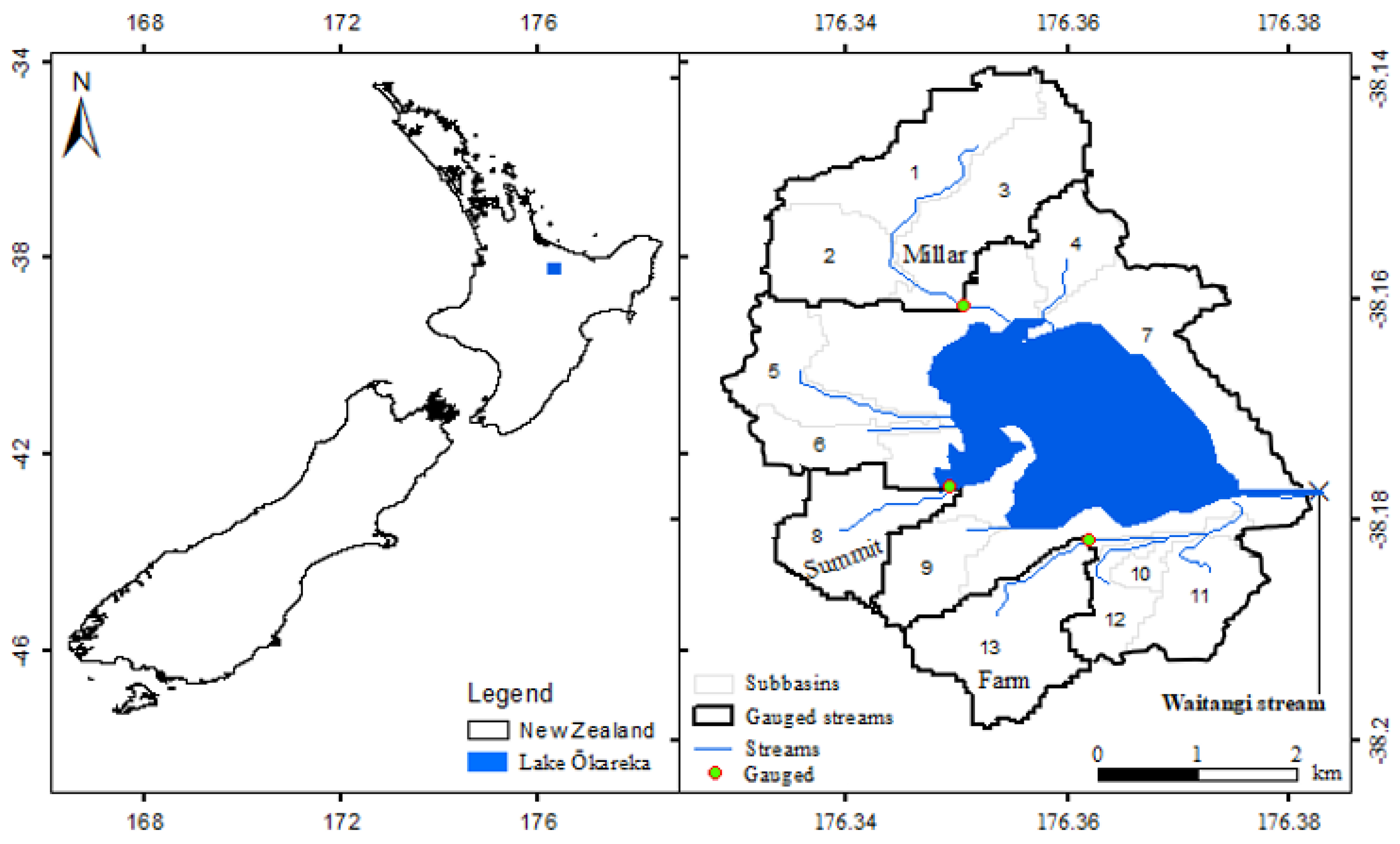
2.1. Study Site

The Ōkareka catchment (Figure 1) is located in the Rotorua District of the North Island of New Zealand. The geology of the area is characterized by volcanic and sedimentary deposits [37] with a series of rhyolitic domes and lava flows flanking the west, south, and east of the lake [38]. The catchment land area is 15 km2 and drains to monomictic, mesotrophic Lake Ōkareka (area ~3.5 km2), which is identified as recreationally and culturally significant. Recent studies of the lake have classified its trophic state as mesotrophic [39] after it was previously assessed to be oligotrophic [40]. The catchment is in a volcanic area and has varying topography, with elevations ranging from 335 to 685 m above mean sea level (amsl). The mean annual precipitation in the area is about 1300 mm, which varies considerably from year to year. The catchment is subjected to a warm temperate climate, with average air temperature, relative humidity, and wind speed of 13.4 °C, 82%, and 3.6 m s−1, respectively (National Climate Database; http://cliflo.niwa.co.nz/ (accessed on 15 June 2023)). Three streams (Millar, Summit, and Farm) are the main surface water inflows to the lake and cover 26, 7, and 10% of the total catchment area, respectively. The only surface outflow from the lake is the Waitangi Stream (mean streamflow 19,400 m3 d−1; Figure 1).

2.2. The Soil and Water Assessment Tool Model

The SWAT is a semi-distributed river basin model that uses inputs of both static landscape and dynamic climate data. Using a digital elevation map, the catchment is divided into smaller sub-catchments, further split into Hydrologic Response Units (HRUs) that have similar land use, soil, and slope characteristics [41]. The model simulates nutrient and sediment transformations and losses for each HRU, and these values are combined to determine the total for each sub-catchment [42]. The predictions are then routed to the appropriate reach and catchment outlet via the channel network [41]. To run the model, daily observed precipitation, temperature, solar radiation, wind speed, and relative humidity are used as input data. The observed climate data used in the model spans from 2002 to 2021.
The SWAT model has a module for nutrient routing that includes organic nitrogen (ORGN), ammonium (NH4-N), and nitrate (NO3-N) [35]. TP is regarded as the sum of mineral phosphorus (MINP) and organic phosphorus (ORGP), and these variables are routed with the nitrogen components and are typically categorized as the particulate and dissolved forms of phosphorus, respectively [20].

2.2.1. SWAT Inputs

A 25 m horizontal resolution Digital Elevation Model was used to delineate the basin and generate stream networks of Lake Ōkareka catchments. Soil type and physicochemical data were obtained from Manaaki Whenua New Zealand Land Resource Inventory (NZLRI) and Digital Soil Map (S-map; http://smap.landcareresearch.co.nz/home (accessed on 15 June 2023)) with similar resolution to the DEM. Land use maps were obtained from New Zealand Land Cover Database v2 (LCDB-2, http://www.lcdb.scinfo.org.nz/about-lcdb (accessed on 15 June 2023)). The landscape data were collected at 25 m resolution, and it provided information on the spatial catchment variation in land use and soil (Table 1). Land use in the Lake Ōkareka catchment area includes native and pine forest, pasture, rangeland, medium density residential areas, and water bodies. The dominant land use in the area is pasture (47%) and forestland (24%) units totaling 71% of the entire area. The other land cover classes are water body (19%), pine plantation trees (6%), medium density residential area (2.6%), and range-brush covered nearly (1.4%).
Data from the Rotorua Airport Automatic Weather Station, which is a part of the National Climatic Database for New Zealand (http://cliflo.niwa.co.nz/ (accessed on 15 June 2023)), were used to provide the necessary inputs for the model such as daily rainfall, temperature, solar radiation, relative humidity, and wind speed. The Bay of Plenty Regional Council collected instantaneous measurements of streamflow and concentrations of NH4-N, NO3-N, TN, and TP for three perennial streams (Millar, Summit, and Farm) near where they enter the lake (Figure 1).

2.2.2. SWAT Model Assessment

To optimize SWAT model parameters, a standalone Calibration and Uncertainty Program, SWAT-CUP, was used [43]. Parameter sensitivity analysis describes how model output varies with changes in parameter value within upper and lower range. Sensitive parameters were identified using Sequential Uncertainty Fitting 2 (SUFI-2) in SWAT-CUP [44], known for its computational efficiency in quantifying the effects of changes in input parameters on model outputs [45]. Streamflow Q and WQ datasets for three observation streams were used for calibration (2002–2005) and validation (2006–2010) years. Calibration of Q and nutrient variables involved parameter sensitivity analysis, following which the model was run for a defined calibration period. The calibration considered the fit between observation and model estimates, the shape of the hydrograph, and the timing of peak flow and nutrient model output. Streamflow was calibrated first followed by water quality variables, and the calibrated model was applied to the validation period without any adjustment of parameters. The performance of the model was evaluated by comparing observation and simulation output of discharge (Q), and NH4-N, NO3-N, TN, and TP concentrations and loads using coefficient of determination (R2) and Nash–Sutcliffe Efficiency (NSE) [46].

2.3. Design of Scenarios

2.3.1. Land Use Change Scenarios

The scenario analyses were implemented to determine the specific sub-catchments and proportions of land conversion that would lead to substantial improvements in streamflow and water quality. Five hydrological simulations were analyzed. The first simulation, which served as a baseline, was from 2002 to 2016 and did not consider any land use changes (referred to as LUC0). The other four simulations (LUC1–LUC4) covered the same period from 2002 to 2016, but factored in land use changes in pasture to forest that occurred after 2011. Land use change effects on flow and nutrient export post 2011 (LUC1) accounted for existing land use change. The remaining three simulation scenarios (LUC2-LUC4) were hypothetical and included: (1) baseline simulation (LUC0), (2) 0.67 km2 existing land use change (LUC1); (3) a further 0.9 km2 LUC in addition to that of LUC1 (LUC2); (4) a further 2.45 km2 of LUC from LUC1 (LUC3); and (5) an additional 4.15 km2 of LUC from LUC1 (LUC4) (Table 2).
The selection of the proportion of land area in the four scenarios LUC1–LUC4 (Table 2) to achieve water quality targets was based on the interplay between the current land use condition, topography, and influence of terrain elevation on soil and nutrient erosion. By carefully assessing the topography and elevation of each specific sub-catchment, we aimed to determine the optimal proportion of land conversion to forest that would yield a significant reduction in streamflow and nutrient loading. The technique allowed us to identify the sub-catchments where afforestation measures would have the most visible impact, particularly in areas with higher pasture coverage.

2.3.2. Climate Change Scenarios

Climate change projections were derived from a global climate model that has been regionally downscaled for New Zealand [20,47]. The projected changes are documented for a set of four representative concentration pathways (RCPs) from the IPCC’s Fifth Assessment [47]. The Representative Concentration Pathway 8.5 (RCP8.5) scenario was chosen to represent an additional radiative forcing of 8.5 W m2 and no major policy-driven climate mitigation actions, leading to high rates of climate change.
The selection of RCP8.5 as a representative concentration pathway was based on several factors specific to New Zealand. In the New Zealand context, RCP8.5 allows for an exploration of the potential impacts of the most extreme emission pathway on various sectors, ecosystems, and communities. It serves as a useful tool for assessing the potential range of future climate change impacts and vulnerabilities. Moreover, RCP8.5 provides a valuable reference point for policymakers and stakeholders to understand the potential risks associated with high-emission scenarios and the urgency of taking mitigation measures.
In terms of relevance and applicability, utilizing RCP8.5 helps us understand the potential range of future climate change impacts, particularly in scenarios where mitigation efforts are limited. It allows us to conduct a comprehensive assessment of potential risks and helps inform adaptation strategies that can be implemented in the face of uncertain future climate conditions. To further support our choice of RCP8.5, we would like to reference the New Zealand Climate Change Projections 2018 report published by the Ministry for the Environment [47], which discusses the use of RCP scenarios, including RCP8.5, in climate change research specific to New Zealand.
Monthly median change factors were generated under the RCP8.5 scenario using linear functions of the global annual mean temperature [20,48]. The projected climate data derived from the downscaled climate projections (Table 3) were used to modify the baseline climate data by adding the minimum and maximum air temperature (Tmin, Tmax) values or by applying a change factor to precipitation (PCP), solar radiation (SLR), and relative humidity (HMD). The future climate datasets were then used as input to the SWAT model to predict future changes in the flow and nutrient loading for all four future land use scenarios.
The climate change simulation (CC0, no LUC) reflected the 2094–2099 climate and considered no land use change, the baseline (LUC0) and the remaining four land use–climate change simulations used the 2094–2099 projected climate and land use change (LUC1–LUC4).
Temporal changes in land use and climate on streamflow and nutrient loads were examined using percentage relative change (Equation (1)) in each variable between a baseline simulation considering no LUC (LUC0) and one that considers land use change, climate change, or a combination of both (Si).
%   Relative   change = 1 S i S 0 × 100

3. Results

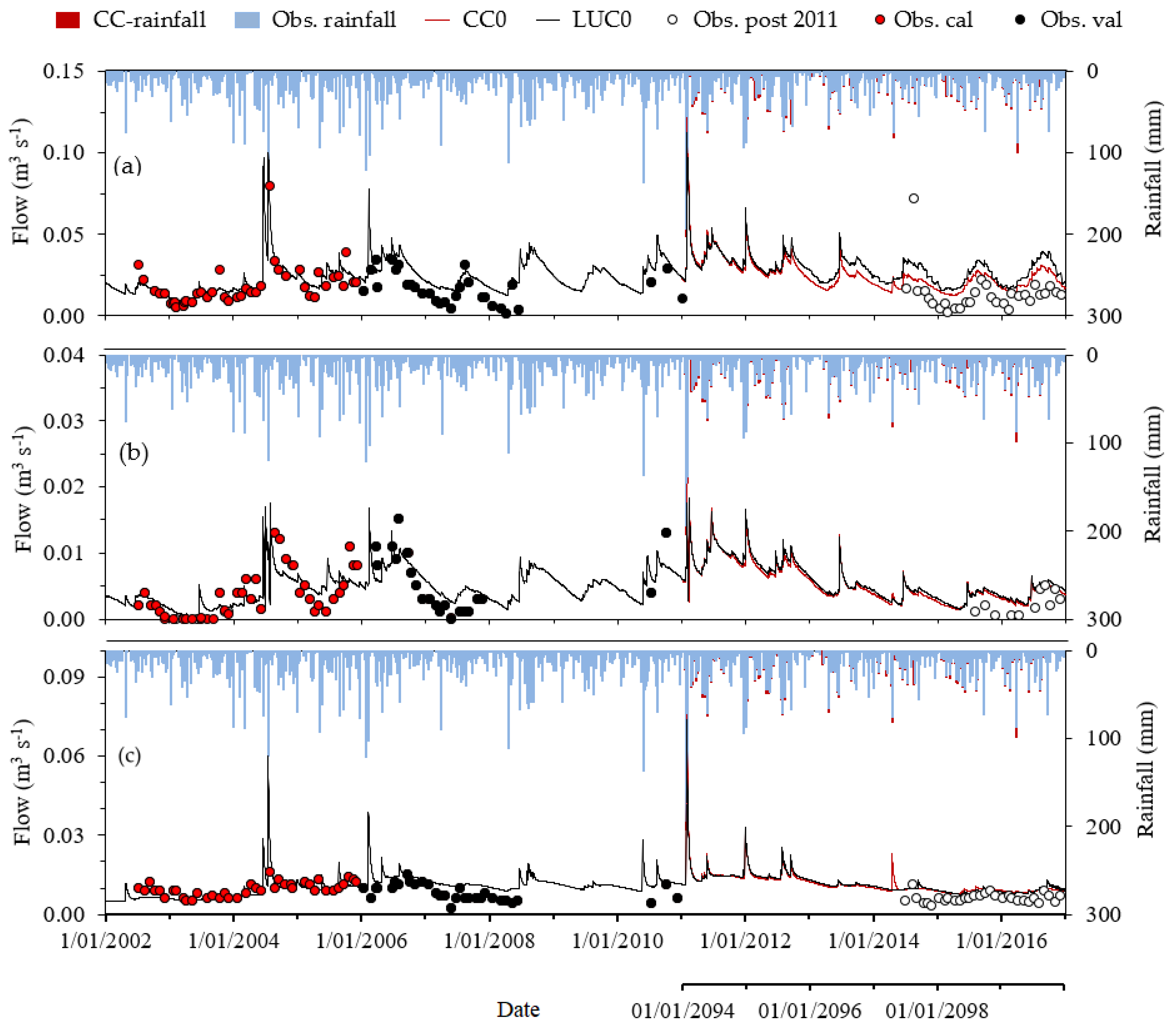
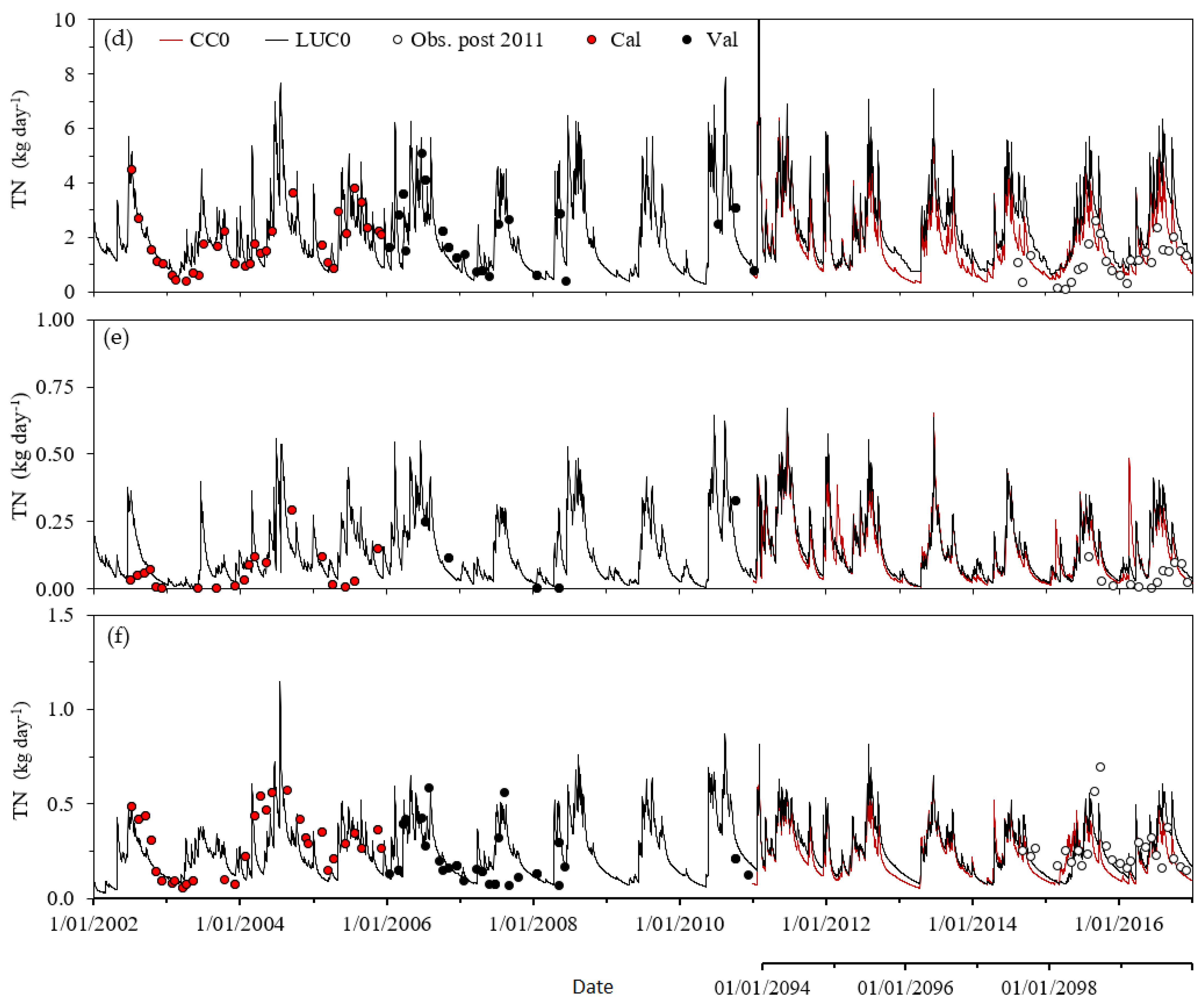
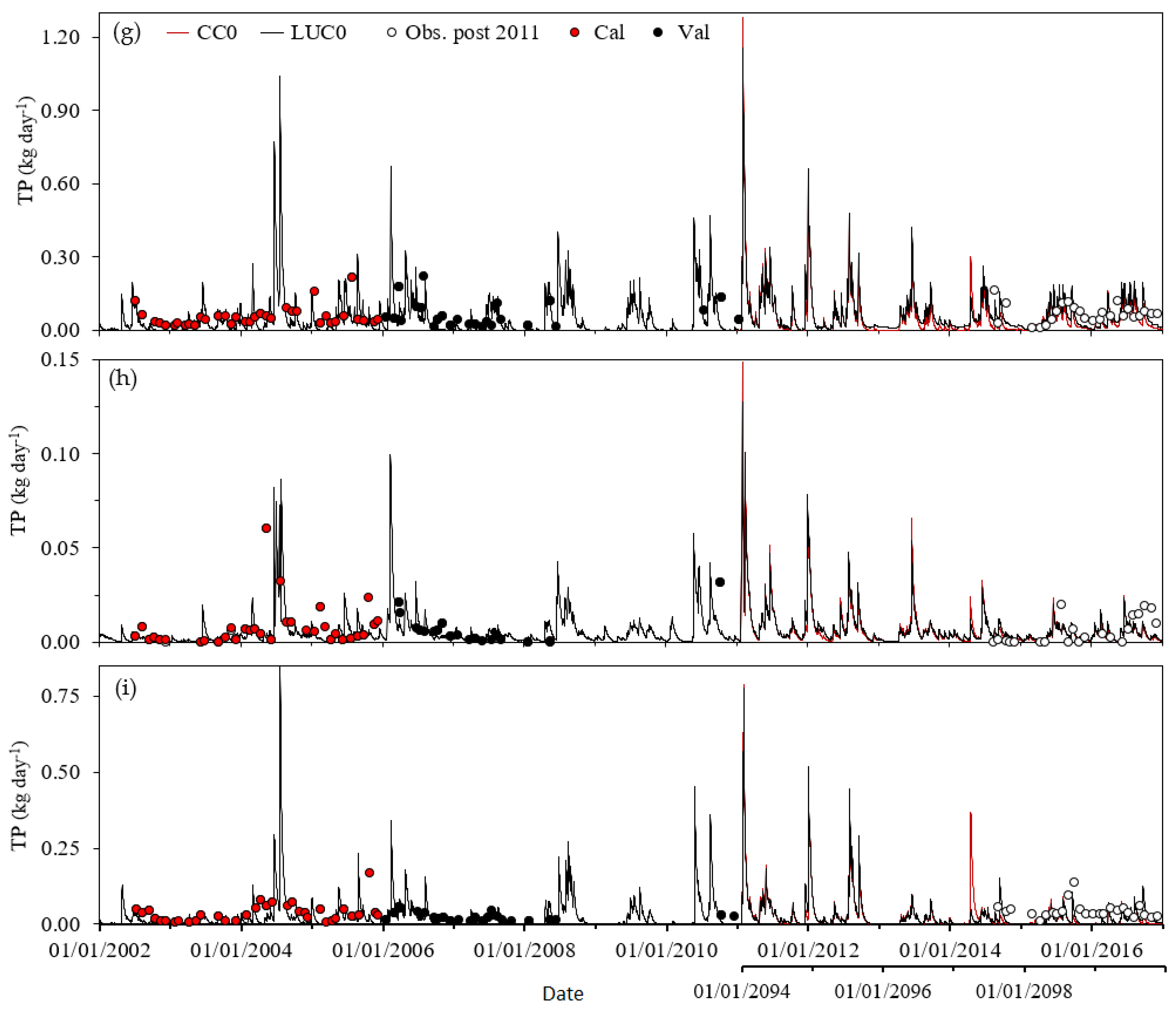
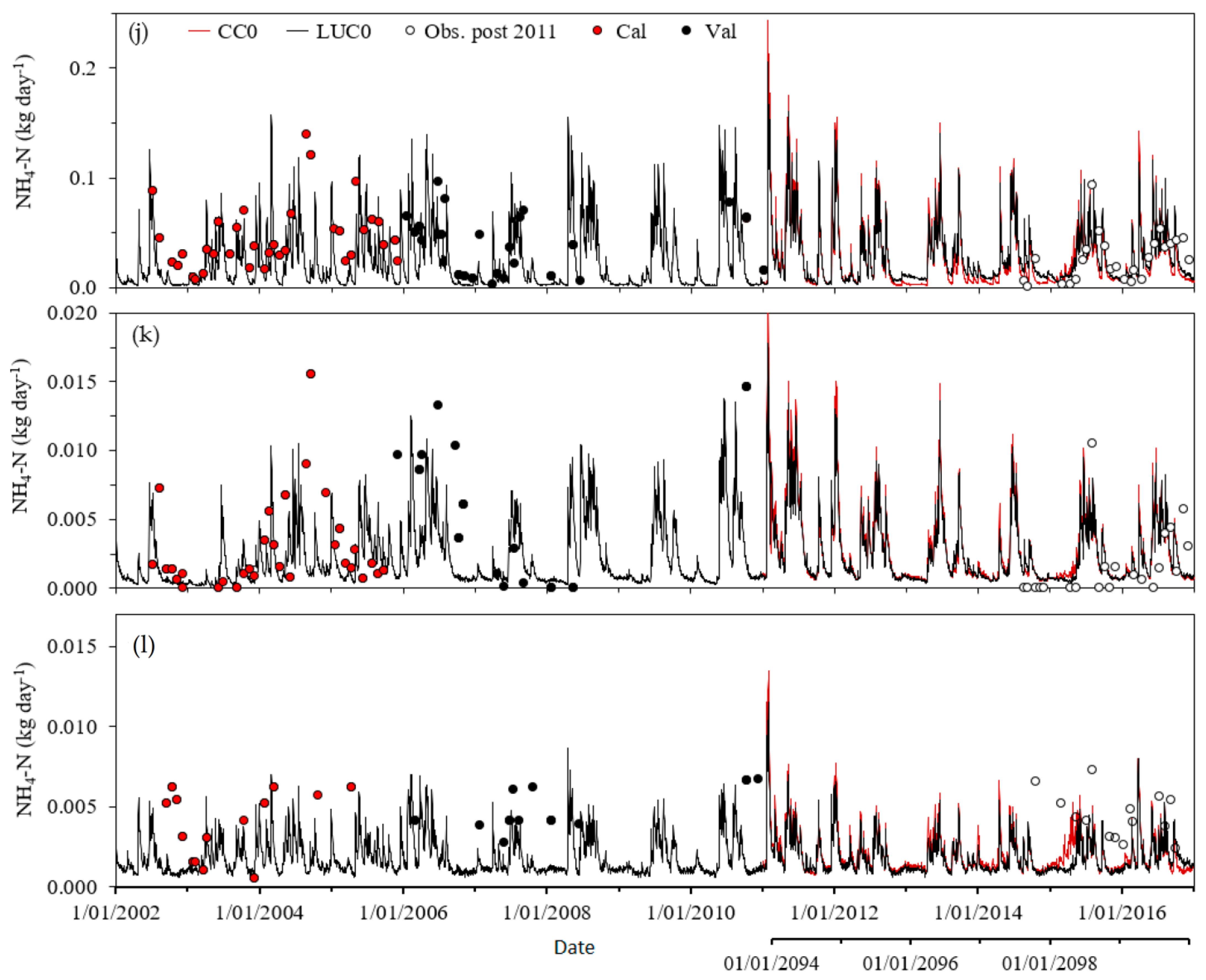
3.1. SWAT Model Calibration and Performance

A sensitivity analysis was conducted for SWAT model parameters and inputs data. Table 4 summarizes the sensitive flow and nutrient related parameters which included average slope (HRU_SLP), initial Soil Conservation Service (SCS) runoff curve number for moisture condition II (CNII), groundwater delay (GW_DELAY), groundwater “revap” coefficient (GW_REVAP), saturated hydraulic conductivity (SOL_K), effective hydraulic conductivity in the main channel (CH_K2), and threshold depth of water in the shallow aquifer required for return flow to occur (GWQMN). Some of these parameters, such as lateral flow travel time (LAT_TTIME) and slope length for lateral subsurface flow (SLSOIL), determined the amount of lateral flow entering the stream reach during quick flow. Catchment slope (HRU_SLP) and available water capacity of the soil layer (SOL_AWC) were sensitive to the base flow simulation as they affect lateral flow within the kinematic storage in the SWAT model [49]. HRU_SLP, a terrain parameter, varies with elevation in the catchment and affects lateral flow within the kinematic storage model in SWAT.
The catchment base flow response was further influenced by the base flow alpha factor (ALPHA_BF) and aquifer percolation coefficient (RCHRG_DP) [50]. Other sensitive parameters included threshold depth of water in the shallow aquifer for “revap” to occur (REVAPMN) and Manning’s “n” value for the main channel (CH_N2). Parameters that control overland processes, such as subbasin average slope length (SLSUBBSN) and Manning’s n value for overland flow (OV_N) were found to be sensitive to varying degrees.
The sensitive TP parameters were organic phosphorus in the base flow (LAT_ORGP), concentration of soluble phosphorus in groundwater contribution to streamflow from the subbasin (GWSOLP), and organic P enrichment ratio (ERORGP).
The most sensitive TN and NO3-N parameters were organic nitrogen in the base flow (LAT_ORGN), rate constant for hydrolysis of organic nitrogen to ammonium–nitrogen in the reach (BC3), nitrate–nitrogen concentration in the shallow aquifer (SHALLST_N), and organic N enrichment ratio (ERORGN). Some parameters tended to influence TN constituent variables more than others. For example, NH4-N was highly sensitive to benthic (sediment) source rate for ammonium–nitrogen in the reach (RS3) and changes in the value of flow parameters.
Observed and simulated streamflow and nutrient load data are indicated in Table 5. Based on R2 values [46], the goodness-of-fit varied from very good (Q) to acceptable and unsatisfactory during calibration (NO3-N, TN, and TP) and validation (NH4-N, NO3-N, TN, and TP), although R2 values for nutrient constituents are in the upper range of values summarized for a number of studies by Arhonditsis and Brett [51]. Model prediction uncertainty was further quantified by NSE values.
The time series plots (Figure 2) represent predicted daily flow and nutrient loads for baseline land use (LUC0, 2002–2016) and baseline climate change simulations (CC0, 2094–2099). A comparison of observed and simulated streamflow for Millar, Summit, and Farm is shown in Figure 2a–c.
The graphical comparison of observed and predicted TN loads (Figure 2d–f) showed a reasonable model fit. Modeled TP (Figure 2g–i) and NH4-N (Figure 2j–l) load predictions aligned well with the seasonal pattern related to high and low flow seasons. NH4-N model estimate for Millar and Summit (Figure 2j–k) showed a good fit during the dry season. While missing the peak for some observations, predictions of NH4-N for Farm catchment (Figure 2l) were stable, with few major over and under predictions.

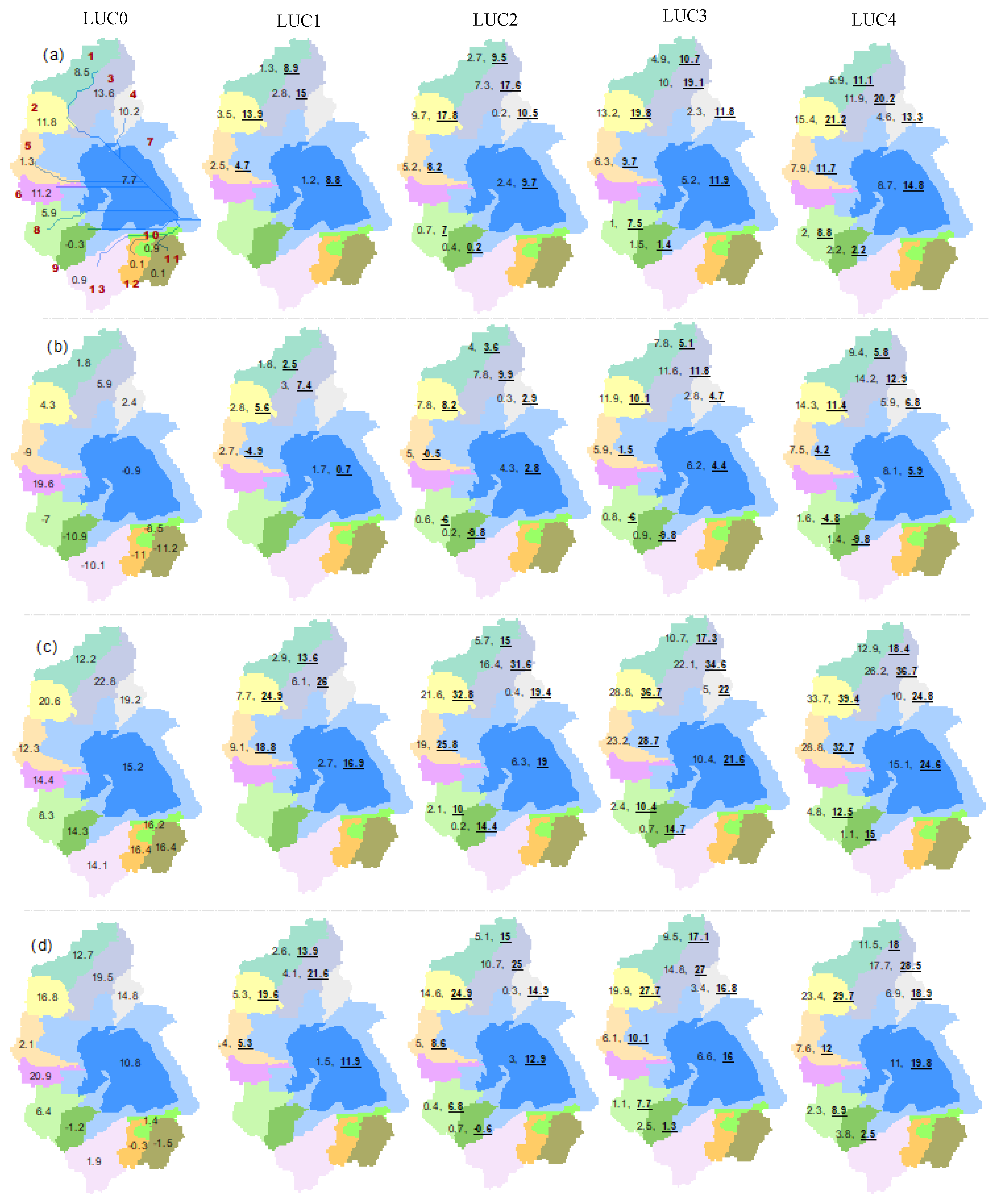
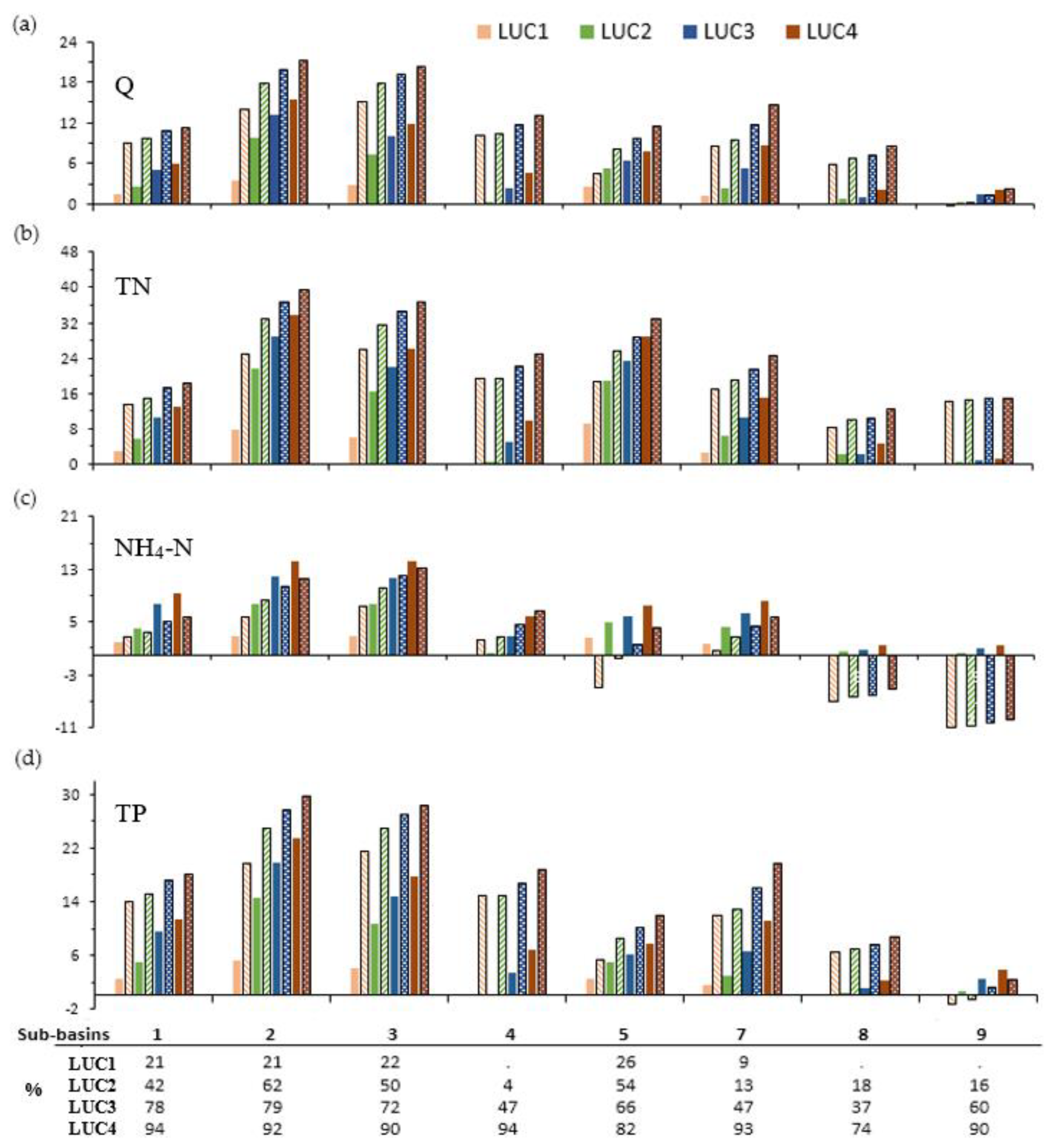
3.2. Modelling Streamflow and Nutrient Loads: Land Use Change Effects

Our model simulations revealed a reduction in stream flow and NH4, TN, and TP load with land use change (LUC), an increase in forest cover (Figure 3). Columns LUC1 through LUC4 show relative changes between baseline simulation (LUC0) and LUC (LUC1–LUC4) and CC scenarios. Considering subbasins 1, for example, in the LUC2 scenario (i.e., relative change in annual average flow and nutrient load between baseline, LUC0 and LUC2 simulations), there was a 2.7, 4.0, 5.7, and 5.1% decrease in Q, NH4-N, TN, and TP by, respectively (column LUC2).
Land use and climate change effects on flow and nutrient loads for other subbasins are also presented. For instance, in subbasin 3, converting 1.1 and 1.32 km2 of pasture to forest during the third (LUC3) and fourth (LUC4) land use change scenario led to a reduction of NH4-N by 11.6% and 14.2%, respectively. Similarly, compared to the baseline simulation, LUC simulations (LUC1–LUC4, column LUC1–LUC4) showed a significant decrease in TP load, with reductions of 4.1%, 10.7%, 14.8%, and 17.7%, respectively, when converting pasture to forest.

3.3. Modelling Streamflow and Nutrient Loads: Land Use–Climate Change Effects

Scenario of flow and nutrient loads for land use–climate change are shown in Figure 3. Figure 3a–d show percent relative change in the predicted annual average flow and nutrient loads between the baseline (LUC0) and climate change-only simulation (CC0) (column LUC0). For example, relative change between LUC0 and CC0 in annual average flow and nutrient loads for subbasin 3 showed a 13.6, 5.9, 22.8, and 19.5% decrease in Q, NH4-N, TN, and TP, respectively (column LUC0, Figure 3a–d).
Bold underlined values in the map (column LUC1–LUC4, Figure 3a–d) show percent relative difference between climate change alone (CC0) and coupled land use and climate change simulations. For subbasin 1, for example, percent relative difference in flow between CC0 and land use–climate change simulations (LU-C1-LUC4) showed 8.9, 9.5, 10.7, and 11.1% reductions, respectively. Streamflow responses for the combined land use–climate change (LU-CC1-LUCC4) compared with CC0 in subbasin 2 showed a 13.9, 17.8, 19.8, and 21.2% reduction, respectively.
Figure 4 displays histograms of the outcomes of applying the relative difference analysis of Equation (1), with the impact of alterations in stream-flow and nutrient loads extending the results presented in Figure 3.
The histogram value above the Cartesian coordinate point (0, 0) indicates a decrease in values of any of the simulated variables. The results revealed a reduction in streamflow and TN and TP loads for all catchments that have undergone land use change. There has been a noticeable change in NH4-N load between the individual and combined simulations. For instance, in subbasin 3, a 5.9% reduction in NH4-N load was observed when comparing the baseline, LUC0, and climate change alone, CC0 simulation. Furthermore, when comparing the four land use climate change scenarios (from LU-CC1 to LU-CC4) with the CC0 results, there was a substantial decrease in NH4-N loads of 7.4%, 9.9%, 11.8%, and 12.9%, respectively. The findings also reveal changes in NH4-N load across some subbasins. For example, in subbasins 8 and 9, a comparison of the LUC-CC and CC0 simulations revealed an increase in NH4-N loads.

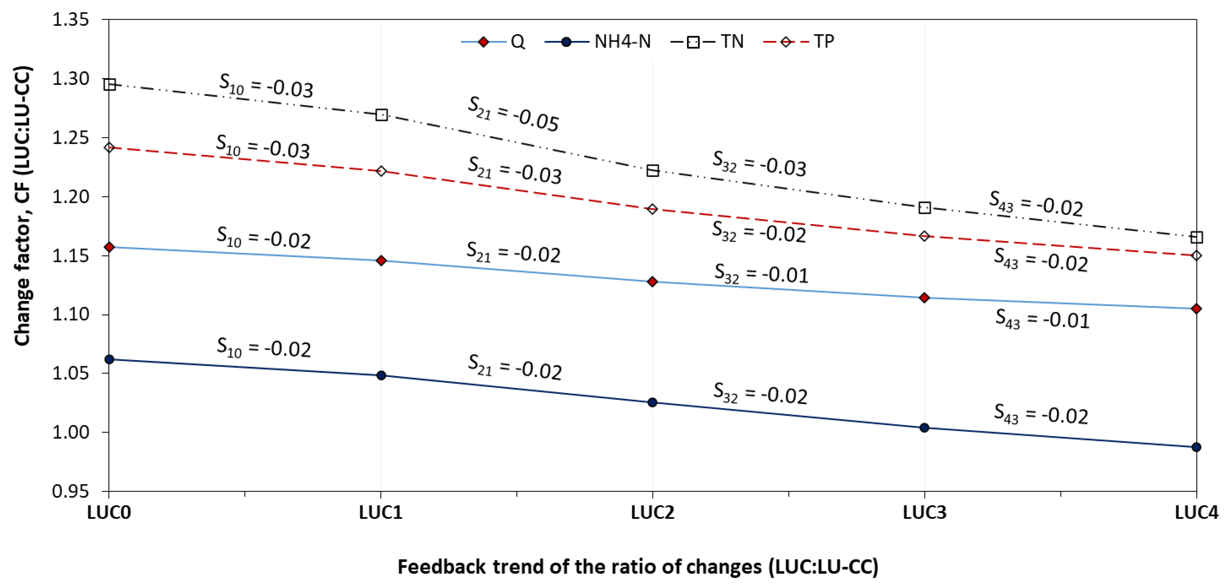
3.4. Combined Effects of Land Use and Projected Climate

Four land use and climate change (LU-CC) scenarios, i.e., LU-CC1 for the first, LU-CC2 for the second, LU-CC3 for the third, and LU-CC4 for the fourth scenario, were used to assess land use change and climate change effects. Figure 5 shows such a case for subbasin 3 with LUC only represented by LUC1–LUC4 and climate change included as LU-CC1, LU-CC2, LU-CC3, and LU-CC4, respectively.
We used change factor (CF) to examine the interactions between LUC and climate for the scenarios compared with the base case (Figure 5). The slope of the line for streamflow (Q), NH4-N, TN, and TP showed relatively small changes between consecutive scenarios. For example, a slope (S21 = −0.02) for streamflow between change factors (LUC1 and LUC2), indicated that land use and climate change are not strongly synergistic, meaning that LU-CC simulations do not significantly enhance the reduction in streamflow and nutrient loads. Based on the change factors (LUC0 to LUC4), it can be concluded that although there has been a reduction in flow and nutrient loads, the combined effects are not noticeably different from the individual LUC effects, indicated by CFs of 1.0 to 1.3. LUC1 through LUC4 showed the existence of co-benefits of LU-CC, but the effect was weaker in the LU-CC than that of LUC alone.

4. Discussion

4.1. Land Use and Climate Change Effects on Streamflow

The impacts of climate and land use changes on catchment hydrology and water quality are significant and well documented [52]. A crucial task in land and water management is identifying the areas where source loadings need to be modified to meet water quality standards in the receiving environment. One potential solution is converting pasture to forest, but it is important to evaluate the effects of these changes on streamflow and WQ. We used high-resolution land use information to identify existing land use changes, and then we assessed the individual and combined impacts of climate and land use change on streamflow and WQ.
Comparing baseline (LUC0) and climate change alone (CC0) simulations in subbasin 3 (Figure 2a, column LUC0), the predicted runoff during CC0 showed a 13.6% decrease that may be attributed mostly to an increase in temperature leading to an increase in evaporation. These results align with IPCC reports [53]. A study in the Ōkāreka region [20] indicated a 2.8% and 1.4% increase in annual mean precipitation and solar radiation. According to their finding, the effect of increased precipitation may have been combated by the reported 0.6% reduction in humidity and 2.7 °C increase in temperature [53]. Our model results can also be linked to statistical relationships of land use and WQ to examine how a future warmer climate might impact nutrient runoff. Other modeling studies assessing simulated climate change impacts on streamflow in the Lake Michigan Basin [54] reported a projected 1.8% decrease in total annual runoff following a 5.1% and 2.6 °C projected increase in total average annual precipitation and average annual air temperature, respectively.
The last four simulation scenarios represented both land use (LUC1–LUC4) and climate change effects. For example, compared to the climate change alone (CC0) and LUC simulations (LUC1–LUC4) in subbasin 3, model results showed a decrease in runoff with increasing rates of land use change, ranging from 15% in LUC1 to 20.2% during LUC4 (Figure 2a, column LUC1–LUC4). The reduction in runoff may be related to one or a combination of the following factors. Canopy effects resulted from the conversion of pasture to forest, which may delay runoff and increase infiltration; the effect of increased rainfall towards producing higher runoff could be counter-balanced by the increased temperature (increase in evapotranspiration), or considering scale issues, land use change effects are more dominant in small, groundwater flow-dominated catchments [55,56,57,58,59]. Other previous studies also support our finding. A study conducted in the northeast edge of the Tibetan Plateau found a 11.28% reduction runoff with climate change [60].

4.2. Modelling Nutrient Flux: Land Use–Climate Change Effects

Comparison of climate and land use–climate change (LU-CC) simulations showed a decrease in TN load. This could be attributed to canopy effects for the land use change and global warming and corresponding increase in temperature for climate change, resulting a reduction in streamflow. The particular SWAT model parameter related to canopy effects is CANMX, the maximum amount of water that can be trapped in the canopy when the canopy is fully developed, which potentially exhibits a strong control of the predicted flow with changes in land use. A modelling study covering 325 km2, of which 63% was agricultural land, reported a 4% decrease in TN load under increased temperature induced by global warming [61].
A comparison of baseline (LUC0) and climate change (CC0) model results in subbasin 3 showed a 22.8% reduction in TN. Combined land use–climate change simulations demonstrated a noticeable reduction in TN load compared to CC0, a value ranging from 26 to 36.7%. This could be attributed to a climate change-induced increase in temperature, resulting in reduced runoff and greater plant uptake capacity with an increase in forest cover. Other studies in the Rotorua catchment reported a 7.6% decrease in TN load under the 2090 climate change [20]. A reduction in TN load was observed in other subbasins that underwent land use change. Thus, the decrease in TN load during the LU-CC simulations may be related to the effect of an increase in temperature. Warming causes an increase in soil temperature, thereby enhancing the plant uptake and denitrification processes. This in turn causes a decrease in major component of TN loads (e.g., NO3–N) and leaching from the catchment. Nguyen et al. [62] highlighted a 21.2% annual average reduction in TN loads with RCP8.5 climate change. Afforestation enhances plant uptake and denitrification processes resulting in a reduction in NO3-N load as a major constituent of TN [63]. A study focusing on climate change impacts on nutrient loads [64] highlighted that a decrease in NO3-N response was evident with the projected changes in climate.
A 19.5% reduction in TP load was observed between LUC0 and CC0. A reduction in TP load with projected climate change has been highlighted by other similar studies. One of this application in a modeling study demonstrated by Robertson et al. [54], indicated simulated climate change impacts on phosphorus loading in the Lake Michigan Basin. They found a projected 3.1% decrease in TP loads to Lake Michigan following a 5.1% and 2.6 °C projected increase in total average annual precipitation and average annual air temperature, respectively. Nguyen et al. [62] highlighted a 28.9.2% average annual reduction in TP loads with climate change during the RCP8.5 climate.
Simulations showed considerable changes in NH4-N load with individual and combined simulations of LUC and CC. For subbasin 3, for example, a 5.9% reduction in NH4-N load occurred with LUC0 and climate change alone and a 7.4 to 12.9% reduction for LU-CC1 and LU-CC4, respectively. The changes in NH4-N may relate to changes in catchment hydrological properties and uncertainty in transferring gauged catchment SWAT model parameter optimal values to ungauged ones. In such a case, biological oxidation of NH4 to NO2 (BC1) and NH4 to NO3 (BC2), and hydrolysis of organic N to NH4 (BC3) were found to influence NH4-N outputs. In addition, NH4-N was highly sensitive to benthic (sediment) source rate for ammonium–nitrogen in the reach (RS3).
For example, subbasins 8 and 9 produced higher NH4-N loads in the CC scenarios, which may relate to changes in catchment hydrological responses of the specific soil dominating the area [65]. An evaluation of the dynamics of NH4-N with a projected increase in precipitation and temperature in the RCP8.5 scenario showed an increase in NH4-N loading associated with increases in temperature. A study by Juang [66] highlighted that increases in temperature can trigger an increase in NH4 fixation that tends to increase the NH4-N flux, reinforced by dehydration and reduced water content in the interlayer of the soil minerals, with more fixed NH4 in the clay fraction. Other studies noted that NH4 fixation could increase with temperature [65,67]. It could also be associated with co-occurrence of hydrological extremes and soil responses [68], and intermittent flash floods may increase NH4+ fixation, which in turn increases NH4-N loading.

4.3. Combined Effects of Land Use and Projected Climate

A reduction in flow and nutrient loads was simulated in both LUC alone and LU-CC model results. In a scenario with substantial LU alteration through afforestation and RCP8.5 climate change, projected streamflow and nutrient loads showed a comparable reduction. Land use change simulations showed a reduction in streamflow and nutrient load, which may have been the result of afforestation and canopy effects that delays runoff and increases infiltration. The decrease in streamflow and nutrient loads can be explained by the combined influence of afforestation and projected increase in temperature. The scenario of an increase in the area of afforestation influences the canopy storage parameter, CANMX, in the SWAT model, which identifies the maximum amount of water that can be trapped when the canopy is fully developed. On the other hand, the rate of reduction in annual average estimates of streamflow and nutrient loads during LU-CC scenarios was not synergistic, although the responses to LUC and CC were somewhat synergistic.
These results also highlight the potential for a reduction in streamflow and nutrient load if recent afforestation regional policies are paired with global efforts to mitigate climate change.

5. Conclusions

Lake Ōkareka is a mesotrophic lake in the temperate Bay of Plenty region in New Zealand, which had previously been in an oligotrophic state. Land use change involving the conversion of pasture to pine plantation has been undertaken to meet nutrient load targets congruent with an oligotrophic state trophic state for the lake. This study therefore represents an important validation for the extent of land use change (LUC) required to meet water quality targets for receiving waters. Our hypothesis was that while increasing forest surface area will reduce nutrient loads, climate change would cause higher precipitation and temperature, leading to increased flow and nutrient loading. We also hypothesized that the effect of LUC may be able to offset climate change. A comparison of simulations based on current and projected climate indicated a reduction in streamflow and nutrient loads using the projected RCP8.5 climate. Further reductions in nutrient loads occurred in simulations that included both land use and climate change effects. Our analyses revealed that the combined impacts of land use and climate change have a greater influence than each individual impact. This study has significant implications as it demonstrates the potential of land use change strategies in mitigating nutrient loads in lakes with water quality issues. Our findings not only offer valuable insights into this specific context but also present a prototype that can be applied to other lake catchments experiencing LUC.

Author Contributions

G.T.A. performed the modeling, conceptualization, formal analysis, data curation, and writing—original draft. B.Y. and D.P.H. made a substantial, direct, and intellectual contribution to the validation, visualization, and supervision of the research. G.T.A. wrote the manuscript with inputs from B.Y. and D.P.H. All authors have contributed toward the study design, methodology, and writing—review and editing. All authors have read and agreed to the published version of the manuscript.

Funding

Gebiaw Ayele received funding from Griffith University through the International Postgraduate Research Scholarship Scheme, Australian Rivers Institute, New Zealand Freshwater Sciences Society (NZFSS) and the V.H. Jolly Travel Award, Australian Freshwater Sciences Society (AFSS) and the Bill Williams Scholarship, and Griffith University International Experience Incentive Scheme (IEIS).

Data Availability Statement

Climate datasets that support the findings of this study are openly available in the NIWA National climate database at https://cliflo.niwa.co.nz/. Streamflow data are available from Bay of Plenty Regional Council Environmental Data Portal at https://envdata.boprc.govt.nz/data and Water quality data were obtained from Bay of Plenty Regional Council. Digital soil data are openly available at http://smap.landcareresearch.co.nz/home, and land use data can be accessed from http://www.lcdb.scinfo.org.nz/about-lcdb).

Acknowledgments

Support for the first author was also through the Lakes380 program (lakes380.com) which is funded by an Endeavour Fund grant from the Ministry of Business, Innovation and Employment. Gebiaw also acknowledges Solomon Demissie and Habtamu Tilahun for every support. We thank the Bay of Plenty Regional Council (BoPRC) and Rotorua District Council (RDC) for providing soil, land use, climate, streamflow, and water quality data. In particular, we thank Andy Bruere and Niroy Sumeran, Max Mackay, Michele Hosking, and Penny MacCormick (BoPRC) and Wang Me (University of Waikato) for providing data to support this study.

Conflicts of Interest

The authors declare that they have no known competing financial interests or personal relationships that could have appeared to influence the work reported in this paper.

Abbreviations

CVP, Central Volcanic Plateau; DEM, digital elevation model; HMD, relative humidity; IPCC, Intergovernmental Panel on Climate Change; LCDB-2, land cover database v2; LUC, land use change; LUC-CC, land use and climate change; NZLRI, New Zealand Land Resource Inventory; NSE, Nash–Sutcliffe efficiency; NO3-N, nitrate; NO2, nitrite; N, nitrogen; NH4-N, ammonium; ORGN, organic nitrogen; PCP, precipitation; P, phosphorus; Q, streamflow; R2, coefficient of determination; SLR, solar radiation; SWAT, Soil and Water Assessment Tool; SWAT-CUP, SWAT-Calibration and Uncertainty Program; SPARROW, SPAtially Referenced Regression On Watershed; SUFI-2, Sequential Uncertainty Fitting 2; TN, total nitrogen; TP, total phosphorus; WQ, water quality.

References

  1. Williamson, C.E.; Dodds, W.; Kratz, T.K.; Palmer, M.A. Lakes and streams as sentinels of environmental change in terrestrial and atmospheric processes. Front. Ecol. Environ. 2008, 6, 247–254. [Google Scholar] [CrossRef]
  2. Moal, M.; Gascuel-Odoux, C.; Ménesguen, A.; Souchon, Y.; Étrillard, C.; Levain, A.; Moatar, F.; Pannard, A.; Souchu, P.; Lefebvre, A. Eutrophication: A new wine in an old bottle? Sci. Total Environ. 2019, 651, 1–11. [Google Scholar] [CrossRef]
  3. Maberly, S.C.; Pitt, J.-A.; Davies, P.S.; Carvalho, L. Nitrogen and phosphorus limitation and the management of small productive lakes. Inland Waters 2020, 10, 159–172. [Google Scholar] [CrossRef]
  4. Leibowitz, S.G.; Wigington, P.J., Jr.; Schofield, K.A.; Alexander, L.C.; Vanderhoof, M.K.; Golden, H.E. Connectivity of Streams and Wetlands to Downstream Waters: An Integrated Systems Framework. J. Am. Water Resour. Assoc. 2018, 54, 298–322. [Google Scholar] [CrossRef]
  5. Fritz, K.M.; Schofield, K.A.; Alexander, L.C.; McManus, M.G.; Golden, H.E.; Lane, C.R.; Kepner, W.G.; LeDuc, S.D.; DeMeester, J.E.; Pollard, A.I. Physical and chemical connectivity of streams and riparian wetlands to downstream waters: A synthesis. JAWRA J. Am. Water Resour. Assoc. 2018, 54, 323–345. [Google Scholar] [CrossRef]
  6. Schindler, D.W.; Carpenter, S.R.; Chapra, S.C.; Hecky, R.E.; Orihel, D.M. Reducing phosphorus to curb lake eutrophication is a success. Environ. Sci. Technol. 2016, 50, 8923–8929. [Google Scholar] [CrossRef]
  7. Abell, J.M.; Özkundakci, D.; Hamilton, D.P. Nitrogen and phosphorus limitation of phytoplankton growth in New Zealand lakes: Implications for eutrophication control. Ecosystems 2010, 13, 966–977. [Google Scholar] [CrossRef]
  8. Smith, V.H.; Wood, S.A.; McBride, C.G.; Atalah, J.; Hamilton, D.P.; Abell, J. Phosphorus and nitrogen loading restraints are essential for successful eutrophication control of Lake Rotorua, New Zealand. Inland Waters 2016, 6, 273–283. [Google Scholar] [CrossRef]
  9. Hamilton, D.P. Land use impacts on nutrient export in the Central Volcanic Plateau, North Island. N. Z. J. For. 2005, 49, 27–31. [Google Scholar]
  10. Filstrup, C.T.; Downing, J.A. Relationship of chlorophyll to phosphorus and nitrogen in nutrient-rich lakes. Inland Waters 2017, 7, 385–400. [Google Scholar] [CrossRef]
  11. Bracken, M.E.; Hillebrand, H.; Borer, E.T.; Seabloom, E.W.; Cebrian, J.; Cleland, E.E.; Elser, J.J.; Gruner, D.S.; Harpole, W.S.; Ngai, J.T. Signatures of nutrient limitation and co-limitation: Responses of autotroph internal nutrient concentrations to nitrogen and phosphorus additions. Oikos 2015, 124, 113–121. [Google Scholar] [CrossRef]
  12. Allgeier, J.E.; Rosemond, A.D.; Layman, C.A. The frequency and magnitude of non-additive responses to multiple nutrient enrichment. J. Appl. Ecol. 2011, 48, 96–101. [Google Scholar] [CrossRef]
  13. Duhon, M.; McDonald, H.; Kerr, S. Nitrogen Trading in Lake Taupo: An Analysis and Evaluation of an Innovative Water Management Policy; Motu Working Paper 14-14; Motu Economic and Public Policy Research: Wellington, New Zealand, 2015. [Google Scholar] [CrossRef]
  14. Burns, N.; McIntosh, J.; Scholes, P. Managing the lakes of the Rotorua district, New Zealand. Lake Reserv. Manag. 2009, 25, 284–296. [Google Scholar] [CrossRef]
  15. BoPRC. Environment Bay of Plenty. 2004. Lake Okareka Catchment Management Plan. Whakatane, NZ. 2004. Available online: https://www.rotorualakes.co.nz/vdb/document/77 (accessed on 21 November 2022).
  16. Elliott, A.H.; Alexander, R.; Schwarz, G.; Shankar, U.; Sukias, J.; McBride, G.B. Estimation of nutrient sources and transport for New Zealand using the hybrid mechanistic-statistical model SPARROW. J. Hydrol. N. Z. 2005, 44, 1–27. [Google Scholar]
  17. Gluckman, P.; Cooper, B.; Howard-Williams, C.; Larned, S.; Quinn, J.; Bardsley, A.; Hughey, K.; Wratt, D. New Zealand’s fresh waters: Values, state, trends and human impacts. In Report for Office of the Priminster’s Chief Science Advisor; Office of the Prime Minister’s Chief Science Advisor: Wellington, New Zealand, 2017; Available online: https://researchspace.auckland.ac.nz/handle/2292/52816 (accessed on 5 December 2022).
  18. Snelder, T.H.; Larned, S.T.; McDowell, R.W. Anthropogenic increases of catchment nitrogen and phosphorus loads in New Zealand. N. Z. J. Mar. Freshw. Res. 2018, 52, 336–361. [Google Scholar] [CrossRef]
  19. Hughey, K.F.; Kerr, G.N.; Cullen, R. Public Perceptions of New Zealand’s Environment: 2016; EOS Ecology: Christchurch, New Zealand, 2016; Available online: https://researcharchive.lincoln.ac.nz/bitstream/handle/10182/3875/?sequence=1:2016 (accessed on 6 December 2022).
  20. Me, W.; Hamilton, D.P.; McBride, C.G.; Abell, J.M.; Hicks, B.J. Modelling hydrology and water quality in a mixed land use catchment and eutrophic lake: Effects of nutrient load reductions and climate change. Environ. Model. Softw. 2018, 109, 114–133. [Google Scholar] [CrossRef]
  21. Williamson, C.E.; Saros, J.E.; Vincent, W.F.; Smol, J.P. Lakes and reservoirs as sentinels, integrators, and regulators of climate change. Limnol. Oceanogr. 2009, 54, 2273–2282. [Google Scholar] [CrossRef]
  22. Pulido-Velazquez, M.; Peña-Haro, S.; García-Prats, A.; Mocholi-Almudever, A.F.; Henríquez-Dole, L.; Macian-Sorribes, H.; Lopez-Nicolas, A. Integrated assessment of the impact of climate and land use changes on groundwater quantity and quality in the Mancha Oriental system (Spain). Hydrol. Earth Syst. Sci. 2015, 19, 1677–1693. [Google Scholar] [CrossRef]
  23. Pachauri, R.K.; Allen, M.R.; Barros, V.R.; Broome, J.; Cramer, W.; Christ, R.; Church, J.A.; Clarke, L.; Dahe, Q.; Dasgupta, P. Climate Change 2014: Synthesis Report. Contribution of Working Groups I, II and III to the Fifth Assessment Report of the Intergovernmental Panel on Climate Change; IPCC: Geneva, Switzerland, 2014. [Google Scholar]
  24. Murray, S.; Foster, P.; Prentice, I. Future global water resources with respect to climate change and water withdrawals as estimated by a dynamic global vegetation model. J. Hydrol. 2012, 448, 14–29. [Google Scholar] [CrossRef]
  25. Messina, N.J.; Couture, R.-M.; Norton, S.A.; Birkel, S.D.; Amirbahman, A. Modeling response of water quality parameters to land-use and climate change in a temperate, mesotrophic lake. Sci. Total Environ. 2020, 713, 136549. [Google Scholar] [CrossRef]
  26. Singh, V.P.; Woolhiser, D.A. Mathematical modeling of watershed hydrology. J. Hydrol. Eng. 2002, 7, 270–292. [Google Scholar] [CrossRef]
  27. Beven, K.; Freer, J. Equifinality, data assimilation, and uncertainty estimation in mechanistic modelling of complex environmental systems using the GLUE methodology. J. Hydrol. 2001, 249, 11–29. [Google Scholar] [CrossRef]
  28. Ayele, G.T.; Teshale, E.Z.; Yu, B.; Rutherfurd, I.D.; Jeong, J. Streamflow and sediment yield prediction for watershed prioritization in the Upper Blue Nile River Basin, Ethiopia. Water 2017, 9, 782. [Google Scholar] [CrossRef]
  29. Devia, G.K.; Ganasri, B.; Dwarakish, G. A review on hydrological models. Aquat. Procedia 2015, 4, 1001–1007. [Google Scholar] [CrossRef]
  30. Vrugt, J.A.; Robinson, B.A.; Vesselinov, V.V. Improved inverse modeling for flow and transport in subsurface media: Combined parameter and state estimation. Geophys. Res. Lett. 2005, 32. [Google Scholar] [CrossRef]
  31. Arnold, J.G.; Williams, J.R.; Maidment, D.R. Continuous-time water and sediment-routing model for large basins. J. Hydraul. Eng. 1995, 121, 171–183. [Google Scholar] [CrossRef]
  32. Arnold, J.G.; Srinivasan, R.; Muttiah, R.S.; Williams, J.R. Large area hydrologic modeling and assessment part I: Model development 1. JAWRA J. Am. Water Resour. Assoc. 1998, 34, 73–89. [Google Scholar] [CrossRef]
  33. Bisantino, T.; Bingner, R.; Chouaib, W.; Gentile, F.; Trisorio Liuzzi, G. Estimation of runoff, peak discharge and sediment load at the event scale in a medium-size Mediterranean watershed using the AnnAGNPS model. Land Degrad. Dev. 2015, 26, 340–355. [Google Scholar] [CrossRef]
  34. Jeong, J.; Kannan, N.; Arnold, J.; Glick, R.; Gosselink, L.; Srinivasan, R. Development and integration of sub-hourly rainfall–runoff modeling capability within a watershed model. Water Resour. Manag. 2010, 24, 4505–4527. [Google Scholar] [CrossRef]
  35. Gassman, P.W.; Reyes, M.R.; Green, C.H.; Arnold, J.G. The soil and water assessment tool: Historical development, applications, and future research directions. Trans. ASABE 2007, 50, 1211–1250. [Google Scholar] [CrossRef]
  36. Me, W.; Abell, J.M.; Hamilton, D.P. Modelling water, sediment and nutrient fluxes from a mixed land-use catchment in New Zealand: Effects of hydrologic conditions on SWAT model performance. Hydrol. Earth Syst. Sci. Discuss. 2015, 12, 4315–4352. [Google Scholar] [CrossRef]
  37. Healy, J. Stratigraphy and chronology of late Quaternary volcanic ash in Taupo, Rotorua, and Gisborne districts. Bull. NZ Geol. Surv. 1964, 73, 88. [Google Scholar]
  38. Nairn, I.; Geology of the Okataina Volcanic Centre, scale 1:50 000. Lower Hutt, New Zealand. GNS Sci. 2002. Available online: https://searchworks.stanford.edu/view/5558763 (accessed on 6 October 2022).
  39. Trolle, D.; Hamilton, D.P.; Pilditch, C.A. Evaluating the influence of lake morphology, trophic status and diagenesis on geochemical profiles in lake sediments. J. Appl. Geochem. 2010, 25, 621–632. [Google Scholar] [CrossRef]
  40. McColl, R. Chemistry and trophic status of seven New Zealand lakes. N. Z. J. Mar. Freshw. Res. 1972, 6, 399–447. [Google Scholar] [CrossRef]
  41. Neitsch, S.L.; Arnold, J.G.; Kiniry, J.R.; Williams, J.R. Soil and water assessment tool theoretical documentation version 2009. Tex. Water Resour. Inst. Tech. Rep. 2011, 406, 1–618. [Google Scholar]
  42. Ayele, G.T.; Kuriqi, A.; Jemberrie, M.A.; Saia, S.M.; Seka, A.M.; Teshale, E.Z.; Daba, M.H.; Ahmad Bhat, S.; Demissie, S.S.; Jeong, J. Sediment yield and reservoir sedimentation in highly dynamic watersheds: The case of Koga Reservoir, Ethiopia. Water 2021, 13, 3374. [Google Scholar] [CrossRef]
  43. Arnold, J.G.; Moriasi, D.N.; Gassman, P.W.; Abbaspour, K.C.; White, M.J.; Srinivasan, R.; Santhi, C.; Harmel, R.; Van Griensven, A.; Van Liew, M.W. SWAT: Model use, calibration, and validation. Trans. ASABE 2012, 55, 1491–1508. [Google Scholar] [CrossRef]
  44. Abbaspour, K.C.; Johnson, C.A.; van Genuchten, M.T. Estimating Uncertain Flow and Transport Parameters Using a Sequential Uncertainty Fitting Procedure. Vadose Zone J. 2004, 3, 1340–1352. [Google Scholar] [CrossRef]
  45. Yang, J.; Reichert, P.; Abbaspour, K.C.; Xia, J.; Yang, H. Comparing uncertainty analysis techniques for a SWAT application to the Chaohe Basin in China. J. Hydrol. 2008, 358, 1–23. [Google Scholar] [CrossRef]
  46. Moriasi, D.N.; Arnold, J.G.; Van Liew, M.W.; Bingner, R.L.; Harmel, R.D.; Veith, T.L. Model evaluation guidelines for systematic quantification of accuracy in watershed simulations. Trans. ASABE 2007, 50, 885–900. [Google Scholar] [CrossRef]
  47. Mullan, B.; Sood, A.; Stuart, S.; Carey-Smith, T. Climate Change Projections for New Zealand: Atmosphere Projections Based on Simulations from the IPCC Fifth Assessment, 2nd ed.; Ministry for the Environment: Wellington, New Zealand, 2018. Available online: https://environment.govt.nz/assets/Publications/Files/Climate-change-projections-2nd-edition-final.pdf (accessed on 6 October 2022).
  48. Touma, D.; Ashfaq, M.; Nayak, M.A.; Kao, S.-C.; Diffenbaugh, N.S. A multi-model and multi-index evaluation of drought characteristics in the 21st century. J. Hydrol. 2015, 526, 196–207. [Google Scholar] [CrossRef]
  49. Sloan, P.G.; Moore, I.D. Modeling subsurface stormflow on steeply sloping forested watersheds. Water Resour. Res. 1984, 20, 1815–1822. [Google Scholar] [CrossRef]
  50. Sangrey, D.A.; Harrop-Williams, K.O.; Klaiber, J.A. Predicting ground-water response to precipitation. J. Geotech. Eng. 1984, 110, 957–975. [Google Scholar] [CrossRef]
  51. Arhonditsis, G.B.; Brett, M.T. Evaluation of the current state of mechanistic aquatic biogeochemical modeling. Mar. Ecol. Prog. Ser. 2004, 271, 13–26. [Google Scholar] [CrossRef]
  52. Osei, M.A.; Amekudzi, L.K.; Wemegah, D.D.; Preko, K.; Gyawu, E.S.; Obiri-Danso, K. The impact of climate and land-use changes on the hydrological processes of Owabi catchment from SWAT analysis. J. Hydrol. Reg. Stud. 2019, 25, 100620. [Google Scholar] [CrossRef]
  53. Stocker, T.F.; Qin, D.; Plattner, G.-K.; Tignor, M.; Allen, S.K.; Boschung, J.; Nauels, A.; Xia, Y.; Bex, V.; Midgley, P.M. IPCC, 2013: Climate Change 2013: The Physical Science Basis: Contribution of Working Group I to the Fifth Assessment Report of the Intergovernmental Panel on Climate Change; Stocker, T.F., Qin, D., Plattner, G.-K., Tignor, M., Allen, S.K., Boschung, J., Nauels, A., Xia, Y., Bex, V., Midgley, P.M., Eds.; Cambridge University Press: Cambridge, UK; New York, NY, USA, 2013; p. 1535. Available online: http://www.cambridge.org/9781107661820 (accessed on 6 October 2022).
  54. Robertson, D.M.; Saad, D.A.; Christiansen, D.E.; Lorenz, D.J. Simulated impacts of climate change on phosphorus loading to Lake Michigan. J. Great Lakes Res. 2016, 42, 536–548. [Google Scholar] [CrossRef]
  55. Woyessa, Y.E.; Welderufael, W.A. Impact of land-use change on catchment water balance: A case study in the central region of South Africa. Geosci. Lett. 2021, 8, 34. [Google Scholar] [CrossRef]
  56. Farley, K.A.; Jobbágy, E.G.; Jackson, R.B. Effects of afforestation on water yield: A global synthesis with implications for policy. Glob. Chang. Biol. 2005, 11, 1565–1576. [Google Scholar] [CrossRef]
  57. Schwärzel, K.; Zhang, L.; Montanarella, L.; Wang, Y.; Sun, G. How afforestation affects the water cycle in drylands: A process-based comparative analysis. Glob. Chang. Biol. 2020, 26, 944–959. [Google Scholar] [CrossRef]
  58. Dons, A. The effect of large-scale afforestation on Tarawera river flows. J. Hydrol. N. Z. 1986, 25, 61–73. [Google Scholar]
  59. Lane, P.N.J.; Best, A.E.; Hickel, K.; Zhang, L. The response of flow duration curves to afforestation. J. Hydrol. 2005, 310, 253–265. [Google Scholar] [CrossRef]
  60. Xue, D.; Zhou, J.; Zhao, X.; Liu, C.; Wei, W.; Yang, X.; Li, Q.; Zhao, Y. Impacts of climate change and human activities on runoff change in a typical arid watershed, NW China. Ecol. Indic. 2021, 121, 107013. [Google Scholar] [CrossRef]
  61. Donnelly, C.; Strömqvist, J.; Arheimer, B. Modelling climate change effects on nutrient discharges from the Baltic Sea catchment: Processes and results. IAHS Publ. 2011, 348, 1–6. [Google Scholar]
  62. Nguyen, H.H.; Recknagel, F.; Meyer, W. Effects of projected urbanization and climate change on flow and nutrient loads of a Mediterranean catchment in South Australia. Ecohydrol. Hydrobiol. 2019, 19, 279–288. [Google Scholar] [CrossRef]
  63. Deng, N.; Wang, H.; Hu, S.; Jiao, J. Effects of afforestation restoration on soil potential N2O emission and denitrifying bacteria after farmland abandonment in the Chinese loess plateau. Front. Microbiol. 2019, 10, 262. [Google Scholar] [CrossRef]
  64. Arheimer, B.; Dahné, J.; Donnelly, C. Climate change impact on riverine nutrient load and land-based remedial measures of the Baltic Sea Action Plan. Ambio 2012, 41, 600–612. [Google Scholar] [CrossRef]
  65. Figueiredo, N.; Carranca, C.; Coutinho, J.; Trindade, H.; Pereira, J.; Marques, P.; de Varennes, A. A climate change scenario and soil ammonium'fixation'during the seasonal rice (Oryza sativa) growth in Portugal under intermittent flooding. Rev. De Ciências Agrárias 2013, 36, 455–465. [Google Scholar] [CrossRef]
  66. Juang, T. Ammonium fixation as affected by temperature and drying-wetting effect in Taiwan soils. Proc. Natl. Sci. Counc. Repub. China. Part B Life Sci. 1990, 14, 151–158. [Google Scholar]
  67. Nieder, R.; Benbi, D.K.; Scherer, H.W. Fixation and defixation of ammonium in soils: A review. Biol. Fertil. Soils 2011, 47, 1–14. [Google Scholar] [CrossRef]
  68. Hien, H.N.; Hoang, B.H.; Huong, T.T.; Than, T.T.; Ha, P.T.T.; Toan, T.D.; Son, N.M. Study of the climate change impacts on water quality in the upstream portion of the cau river basin, vietnam. Environ. Model. Assess. 2016, 21, 261–277. [Google Scholar] [CrossRef]
Figure 1. Location map of the study area. Left: location of Lake Ōkareka in New Zealand. Right: Lake Ōkareka (shaded) and its catchment, showing the major sub-catchments (numbered 1 to 13) including the gauged surface streams (circles filled green with red boundary) for Millar Road, Summit Road, and Farm.
Land 12 01326 g001
Figure 2. Comparison of observed and predicted daily streamflow for three surface streams: Millar (a), Summit (b), and Farm (c). TN load for Millar (d), Summit (e), and Farm (f) and TP load for Millar (g), Summit (h), and farm (i). Daily NH4-N load for Millar (j), Summit (k), and farm (l) streams. The schematic comparison between daily observed and simulated values are indicated by red circles for calibration (2002–2005), black circles for validation (2006–2010), and black hollow circles for periods where there has been land use change (2011–2016) and predicted climate change effects (2094–2099). LUC0 and CCo denote baseline simulation and climate change alone simulations, respectively, and obs., cal., and val. represent observation, calibration, and validation, respectively.
Land 12 01326 g002aLand 12 01326 g002bLand 12 01326 g002cLand 12 01326 g002d
Figure 3. Distribution maps of annual average relative difference in streamflow: (a) NH4-N, (b) TN (c), and TP (d). Column LUC0 (ad) shows percent relative changes in the predicted annual average flow and nutrient load between baseline (LUC0) and climate change alone (CC0) simulations. Relative change between baseline (LUC0) and LUC simulations (LUC1–LUC4) is indicated by columns LUC1–LUC4. Bold underlined values in the map (values after comma) show percent relative difference between climate change alone (CC0) and land use-CC simulations. Relative change computation is as presented in Equation (1) and subbasin numbers are presented in bold red, column LUC0. Subbasins that were not influenced by any land use change scenario are left unlabeled.
Land 12 01326 g003
Figure 4. Effect of LU and LU-CC on streamflow (Q) (a), TN (b), NH4-N (c), and TP (d) load under LUC alone past (solid) and future (hatched) simulations (LUC1–LUC4). The value of the histogram above (0, 0) in the Cartesian coordinate denotes a reduction in prediction of any of the simulated variables (streamflow, NH4-N, TN, and TP) and the table represents percentage of pasture area converted to forest.
Land 12 01326 g004
Figure 5. Feedback between land use and climate change for subbasin 3 in the Lake Ōkareka catchments. Y-axis is a change factor (CF); ratio of land use change alone (LUC1–LUC4) predictions to land use–climate change model outputs (LU-CC1–LU-CC4) is indicated by LUC1 to LUC4; and ratio of baseline simulation to climate change alone simulation (LUC0:CC0) is indicated by LUC0 for streamflow, NH4-N, TN, and TP. X-axis shows the trend of feedback as represented by the slope (s) of the line for each variable.
Land 12 01326 g005
Table 1. Data sources and descriptions used to configure SWAT model.
DataApplicationData Use and DescriptionSource
Meteorological data Meteorological forcingDaily max. and min. temperature, humidity, radiation, wind speed, and precipitation.Rotorua Airport Automatic Weather Station, National Climate Database (available at: http://cliflo.niwa.co.nz/ (accessed on 15 June 2023))
DEM and digitized stream networkCatchment delineation25 m resolution to define slope classes.Bay of Plenty Regional Council (BoPRC)
Land useTo define HRUs25 m resolution, 6 basic land-cover classes.New Zealand Land Cover Database Version 2; BoPRC
Soil characteristicsTo define HRUs25 m resolution, 9 soil types.New Zealand Land Resource Inventory and Digital Soil Map (http://smap.landcareresearch.co.nz (accessed on 15 June 2023))
Table 2. Land use change in the Ōkareka subbasin; baseline (LUC0) and four scenarios of land use change (LUC1–LUC4).
SubbasinReach Area
(km2)
Areas Converted from Pasture to Forest (km2)
LUC0LUC1LUC2LUC3LUC4
11.34-0.030.050.100.10
22.27-0.160.470.600.70
33.84-0.130.280.400.50
40.60-0.000.010.100.20
50.86-0.160.330.400.50
718.42-0.200.271.002.00
81.11-0.000.050.100.20
90.67-0.000.110.400.60
Total area afforested (km2)-0.671.563.104.80
Table 3. Monthly median values of change increments (+) for minimum (Tmin) and maximum temperature (Tmax), change factors (*) for precipitation (PCP), solar radiation (SLR), and humidity (HMD) used to generate the 2094–2099 RCP8.5 climate relative to the 2005 to 2010 baseline climate. The projected annual precipitation (mm) is also presented.
VariableJanuaryFebruaryMarchAprilMayJuneJulyAugustSeptemberOctoberNovemberDecember
PCP (*)1.051.061.1271.0691.0341.0361.0221.0490.9590.9220.9950.983
SLR (*)1.0111.0071.0071.0121.0181.0221.0091.011.0241.0281.0141.01
Tmax (+)3.13.23.12.82.82.52.82.62.72.62.52.5
Tmin (+)3.22.93.12.72.62.72.62.72.22.42.32.6
HMD (*)0.9930.9861.00.9930.9960.9970.9971.00.9990.9940.9890.988
Projected annual precipitation
Year 2090209120922093209420952096209720982099
Rainfall 1137.61521.51198.91465.72039.91287.91210.61046.31097.41296.3
Table 4. Sensitive SWAT model parameters for streamflow (Q), total nitrogen (TN), and total phosphorus (TP) as indicated in SWAT-CUP. The ‘v’ before the parameter indicates replacement of default value by the calibrated values, the ‘a’ denotes addition of the calibrated value to the model default, and ‘r’ is for relative change.
QTNTP
v__LAT_TTIME.hruv__LAT_ORGN.gwv__LAT_ORGP.gw
v__GWQMN.gwv__ERORGN.hruv__GWSOLP.gw
a__SLSOIL.hruv__SHALLST_N.gwV_ERORGP.hru
a__CANMX.hruv__BC3.swq
r__HRU_SLP.hru
v__ALPHA_BF.gw
v__RCHRG_DP.gw
v__CH_K2.rte
Table 5. Model performance statistics (R2 and NSE) for calibration (2002–2005) and validation (2006–2010) for streamflow (Q), nitrate (NO3-N), ammonium (NH4-N), total nitrogen (TN), and total phosphorus (TP).
Calibration
StreamsMillarSummitFarm
VariableQNO3NH4TNTPQNO3NH4TPQNO3NH4TNTP
UnitML d−1g d−1g d−1g d−1g d−1ML d−1g d−1g d−1g d−1ML d−1g d−1g d−1g d−1g d−1
Mean (obs)1.571390601860600.4353.463.228.140.82165.3112.91309.2726.13
Mean (sim)1.9211003018301300.3883.562.015.830.75169.871.68211.3312.24
R20.770.590.530.440.300.730.630.260.140.480.510.030.360.26
NSE0.500.360.200.40−21.630.620.470.16−0.44−0.10.47−0.320.09−0.49
Validation
StreamsMillarSummitFarm
VariableQNO3NH4TNTPQNO3NH4TPQNO3NH4TNTP
UnitML d−1g d−1g d−1g d−1g d−1ML d−1g d−1g d−1g d−1ML d−1g d−1g d−1g d−1g d−1
Mean (obs)1.421840402390600.47101.563.587.150.69141.2518.48224.7123.26
Mean (sim)1.731240301990300.51108.522.395.991.02177.251.63224.9616.07
R20.730.300.200.420.510.670.510.030.030.460.340.010.580.47
NSE0.580.02−0.340.340.140.580.5−0.2−0.21−1.170.21−0.140.57−0.21
Disclaimer/Publisher’s Note: The statements, opinions and data contained in all publications are solely those of the individual author(s) and contributor(s) and not of MDPI and/or the editor(s). MDPI and/or the editor(s) disclaim responsibility for any injury to people or property resulting from any ideas, methods, instructions or products referred to in the content.

