Article

Impact of Drought on Land Productivity and Degradation in the Brazilian Semiarid Region

by
Franklin Paredes-Trejo
1,2,*,
Humberto Alves Barbosa
2,
Gabriel Antunes Daldegan
3,
Ingrid Teich
4,5,
César Luis García
5,
T. V. Lakshmi Kumar
6 and
Catarina de Oliveira Buriti
7
1
Department of Civil Engineering, San Carlos Campus, University of the Western Plains Ezequiel Zamora, Cojedes 2201, Venezuela
2
Laboratório de Análise e Processamento de Imagens de Satélites (LAPIS), Institute of Atmospheric Sciences, A. C. Simões Campus, Federal University of Alagoas, Alagoas 57072-900, Brazil
3
Betty and Gordon Moore Center for Science, Conservation International, 2011 Crystal Drive, Suite 600, Arlington, VA 22202, USA
4
Centre for Development and Environment (CDE)-WOCAT, University of Bern, 63012 Bern, Switzerland
5
Food and Agriculture Organisation of the United Nations, Viale delle Terme di Caracalla, 00153 Rome, Italy
6
Atmospheric Science Research Laboratory, Department of Physics, SRM Institute of Science and Technology, Chennai 603203, India
7
National Semiarid Institute (INSA), Ministry of Science, Technology and Innovations (MCTI), Campina Grande 58429-970, Brazil
*
Author to whom correspondence should be addressed.
Land 2023, 12(5), 954; https://doi.org/10.3390/land12050954
Submission received: 10 March 2023 / Revised: 12 April 2023 / Accepted: 24 April 2023 / Published: 25 April 2023

Abstract

:
The Brazilian semiarid region (BSR) has faced severe drought over the last three decades, which has led to a significant decline in land productivity, posing a considerable threat to food security and the local economy and communities. The United Nations Convention to Combat Desertification (UNCCD) has proposed the use of Earth observation-derived vegetation indices for monitoring land degradation across regions. In this study, we aim to evaluate three comprehensive UNCCD-recommended land productivity dynamic (LPD) approaches in the BSR by utilizing the standardized precipitation–evapotranspiration index (SPEI) at 12-month time scales as a benchmark drought index obtained from ground-based measurements. Our findings indicate that the LPD methods utilizing residual trends analysis (RESTREND), Trends.Earth (TE), and the Food and Agricultural Organization’s World Overview of Conservation Approaches and Technologies (FAO-WOCAT) are best suited for identifying degraded land areas in the BSR region compared to other approaches. However, it is advisable to use these methods with caution, since they do not fully capture the impact of drought on vegetation and may result in underestimating the extent of degraded areas. The RESTREND-based LPD, TE, and FAO-WOCAT estimate that the BSR region reached 213,248 km2, 248,075 km2, and 246,783 km2 of degraded land, respectively, between 2001 and 2015. These findings may be valuable for decision-makers involved in land management and conservation efforts in the Sertão region of Brazil.

1. Introduction

Droughts are a common type of extreme weather event that can impact large areas globally [1,2]. Evidence suggests that climate change may be contributing to the increased frequency and severity of droughts in Europe [3], the United States [4], South America [5], including Brazil [6,7]. Droughts are becoming a major concern in Brazil due to their significant impacts on society [8,9]. Climate projections indicate that droughts and higher temperatures will likely increase in the Brazilian semiarid region (BSR) [10,11].
The BSR is an economically and socially disadvantaged region located in northeast Brazil, with a history of severe drought conditions, making it a drought hotspot [12]. The shortage of precipitation impacts subsistence agriculture, which relies heavily on rainfall, particularly in drought years [13]. Drought and high temperatures can lead to the loss of rainfed crops, reduced storage in lakes and reservoirs, and conflicts between water users [14].
Drought in BSR arises from complex interactions between large-scale ocean–atmosphere modes [11] exacerbated by anthropogenic factors, including deforestation and agricultural expansion [15]. These factors gradually and subtly contribute to precipitation deficits, which in turn have far-reaching and intricate socioeconomic consequences [16]. Four main types of droughts are recognized in the scientific literature: meteorological, hydrological, agricultural, and socioeconomic [17]. These stages represent the progressive impact of drought on human and natural systems [18]. Drought indices based on hydroclimatic and biophysical measurements are used to measure the manifestation of each type of drought over a given period, including its onset, intensity, spatial extent, duration, and cessation [19].
Assessing drought in the BSR can be challenging due to the limited availability of ground monitoring stations that measure hydroclimatic variables such as precipitation [20]. However, advances in remote sensing technology have improved drought assessment and monitoring using Earth observation-based drought indices, which provide a consistent and comprehensive data record over time, even in remote areas [21]. Recent studies in the BSR have shown that satellite-based drought indices, such as the standardized precipitation and evapotranspiration index (SPEI), can effectively complement ground-based measurements in capturing drought characteristics in the region [22].
Recurrent drought cycles in semiarid regions may trigger cascading effects that exacerbate land degradation [23,24], with serious consequences for food security and the functioning of ecosystem processes [25,26]. Land degradation, as defined by the United Nations Convention to Combat Desertification (UNCCD), is the reduction of a land’s biological productivity due to biophysical and anthropogenic pressures [27,28]. To assess land degradation globally, the UNCCD has adopted Sustainable Development Goals (SDG) indicator 15.3.1, a binary indicator of land condition (degraded/not degraded) calculated by integrating three spatially explicit sub-indicators using a one-out-all-out (1OAO) method, in which a negative change in any one of the sub-indicators is interpreted as degradation [29,30].
The three sub-indicators comprising SDG Indicator 15.3.1 are: (i) trends in land cover, measured through land cover maps, a land cover transition matrix, and a legend harmonized with Intergovernmental Panel on Climate Change (IPCC) classes; (ii) trends in carbon stocks, measured by changes in soil organic carbon (SOC) using soil maps of carbon content or SOC estimates from the SoilGrids250 m product, land cover change, and climate/land cover change factors following IPCC guidelines (Tier 1); (iii) trends in land productivity, assessed through changes in total above-ground net primary productivity (NPP) estimated using time series of the normalized difference vegetation index (NDVI) integrated during each growing season as a proxy for NPP [31].
Currently, the UNCCD endorses three distinct geospatial datasets representing land productivity trends, each based on NDVI at the pixel level. These datasets are employed to assess land productivity dynamics (LPD) through three approaches: LPD from Trends.Earth (TE), LPD from the Joint Research Center (JRC-LPD), and LPD from the Food and Agriculture Organization’s World Overview of Conservation Approaches and Technologies (FAO-WOCAT LPD). The default global dataset for land productivity utilized by the UNCCD is the JRC-LPD. The TE method involves three metrics: (i) trend, which assesses the trajectory of annually-integrated productivity change over a 16-year moving window through the application of linear regression and the Mann–Kendall nonparametric significance test of the slope of the NDVI; negative significant changes are interpreted as degraded land, while positive ones indicate not degraded land; (ii) state, which compares the mean NDVI of the three most recent years to the preceding 13 years using cut-off values based on 10 percentile classes of the NDVI frequency distribution; a class change less than −2 is interpreted as degraded land, one greater than 2 indicates an improved land condition, while one between −2 and +2 is considered stable; (iii) performance, which compares the productivity levels of each land unit within the land cover/ecosystem functional unit (LCEU) using the ratio of the mean observed NDVI to the maximum for other pixels within the same LCEU; a ratio less than 0.5 is reported as degraded land, while a ratio greater than or equal to 0.5 is flagged as stable land. The three metrics are then combined using a lookup table to categorize degradation into five levels: declining, moderate decline, stressed, stable, and increasing [32].
The JRC-LPD approach uses annual aggregations of NDVI values to estimate the tendency of change in land productivity (long-term change map) and the current status map, which are then combined per pixel to generate a categorical map with the same LPD classes as the TE method. The long-term change map is produced by integrating three categorical metrics: the steadiness index, baseline level of productivity, and change in the state of productivity. The steadiness index is calculated by combining two sub-metrics: (i) the slope determined by fitting a linear regression model on the annual NDVI time series, and (ii) the net change in productivity level estimated using the multi-temporal image differencing method [33]. The baseline level of productivity (initial biomass) is the NDVI average for the first three years, categorized into three classes (low, medium, high) using a quantile categorization strategy or predefined thresholds. The change in the state of productivity (state) assesses the percentile jump between the productivity level at the beginning and end of the NDVI time series using the same quantile-based method as for initial biomass [34]. The current status map is produced using a similar framework to the performance metric in the TE.
The FAO-WOCAT approach is a hybrid model that integrates elements from both the JRC-LPD and TE methods [35]. FAO-WOCAT involves the computation of linear trends in annual NDVI time series through nonparametric techniques and changes in performance with respect to the current state, considering the initial biomass value [36]. This feature facilitates the adjustment of parameters to more accurately correspond with the conditions encountered within the study area.
Prolonged drought in the BSR can negatively impact ecosystems due to their reliance on rainfall, resulting in a long-term decrease in NDVI [37,38]. In this context, it is reasonable to expect that the three LPD approaches recommended by the UNCCD could identify a significant proportion of land degradation caused by drought rather than direct human impacts [39].
Unlike other approaches, the TE method offers three correction methods to minimize the influence of climate on LPD. The first method, rain use efficiency (RUE), calculates the ratio of annual NDVI to annual precipitation, and a non-parametric Wilcoxon’s rank sum test is applied to the linear trend of RUE over time. Negative RUE trends are interpreted as potential land degradation, while positive trends indicate potential land improvement [40]. The second method, residual trend analysis (RESTREND), is a variant of RUE that involves predicting annual NDVI based on historical annual rainfall, calculating the difference between the observed and predicted NDVI (residual), and applying a non-parametric Mann–Kendall trend test to the linear trend line fitted to the residuals. Negative trends in the residuals are interpreted as non-climatically related productivity change [41]. The third method, water use efficiency (WUE), calculates the ratio of annual NDVI to annual evapotranspiration (ET) and follows the same steps and interpretation as RUE [42,43].
Although some studies have employed methodologies similar to those proposed by the UNCCD to evaluate LPD in North America [44] and Asia [45], these have not been adopted by the scientific community as a standard reference. In the context of LPD, Conservation International designed Trend.Earth, a free and open-source tool, to evaluate land productivity dynamics using the three approaches recommended by the UNCCD [46]. This tool was developed as part of the project “Enabling the use of global data sources to assess and monitor land degradation at multiple scales” funded by the Global Environment Facility [47].
To our knowledge, no study has investigated the reliability of the three LPD approaches recommended by the UNCCD and climate correction methods in the BSR. In this study, we aim to address the existing knowledge gap within the BSR by (1) investigating the similarity in response of the three LPD approaches endorsed by UNCCD (i.e., TE, JRC-LPD, and FAO-WOCAT) under distinct precipitation regimes; (2) assessing the impact of drought severity, as quantified by the SPEI on an annual basis, on the detection of degraded areas when utilizing the three climate-corrected LPD approaches (i.e., RUE, RESTREND, and WUE); and (3) evaluating the performance of all UNCCD-recommended LPD approaches against two established benchmarks in terms of hit rate to determine the most appropriate method for detecting degraded areas in this semiarid region. Previous research demonstrates that vegetation in semiarid regions can exhibit a strong coupling with precipitation and a delayed response to drought, which may lead to misinterpretation of degradation [25,48,49]. In this context, the SPEI is often used to assess the severity of drought as a proxy for long-term drought conditions [22,50]. We hypothesize that the LPD approaches might incorrectly identify non-degraded regions as degraded land in the BSR as a result of these characteristics.

2. Materials and Methods
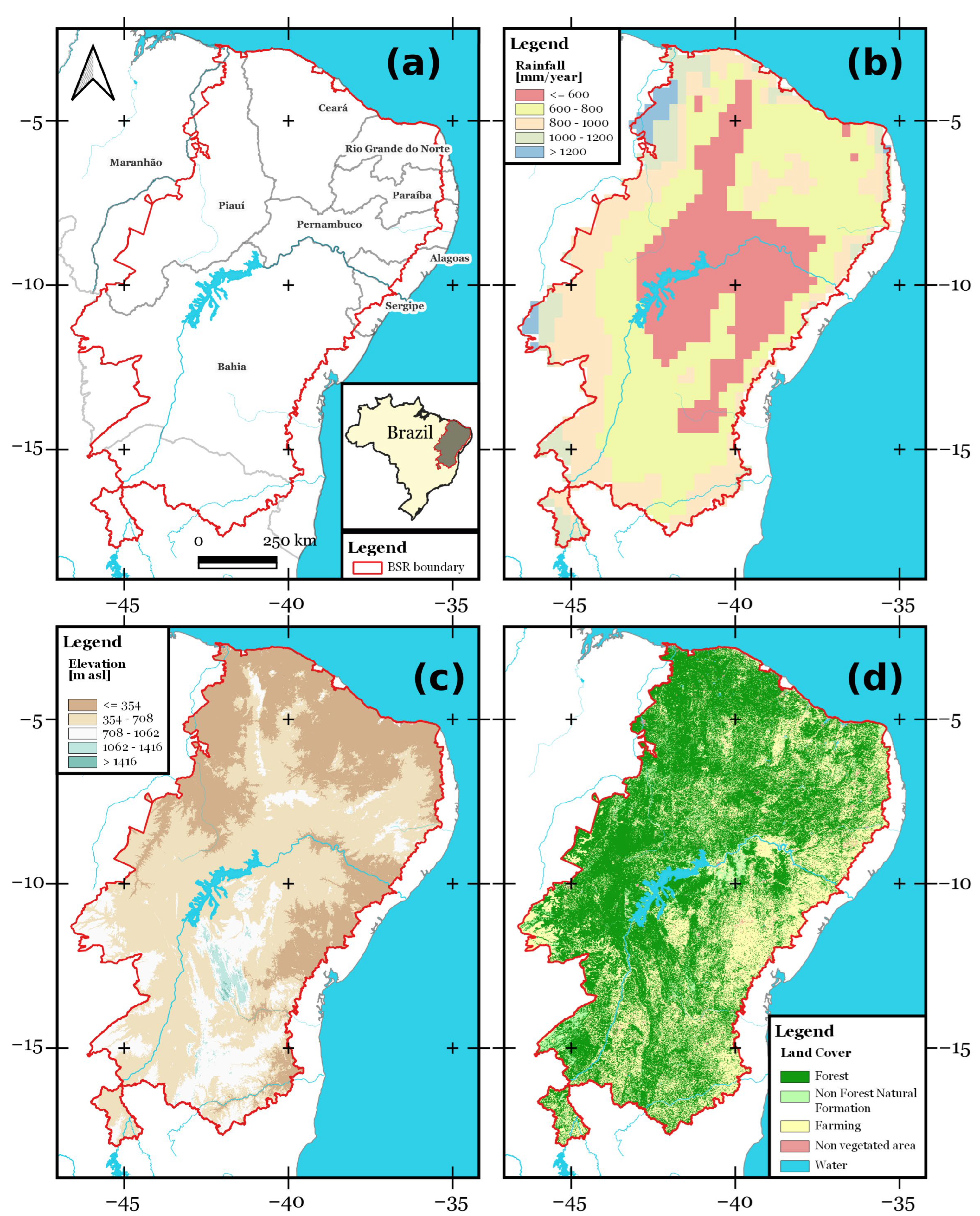
2.1. Study Area

The study area is in northeast Brazil (NEB), covering approximately 1.13 million km2 between latitudes 2.7–17.9° S and longitudes 35.3–46.6° W (Figure 1a). It is known as the Sertão region. The BSR has more than 27 million inhabitants in 10 federal states and 1262 municipalities. It is characterized by rich biodiversity, diverse landscapes, topography, and rainfall patterns [51,52]. The climate is predominantly tropical savannah (Aw), with mean air temperatures ranging from 17–28 °C and annual rainfall averaging 744 mm (Figure 1b). Precipitation is influenced by moisture transport from the Atlantic Ocean, which is modulated by sea surface temperature (SST) anomalies and El Niño Southern Oscillation (ENSO) [6,14]. The elevation of the region increases from the northern lowlands to the Serra do Sincorá, reaching elevations of over 1800 m above sea level (Figure 1c). Forests are the dominant land cover, comprising about 60% of the region’s surface (Figure 1d).

2.2. Datasets

2.2.1. Standardized Precipitation Evapotranspiration Index (SPEI)

The SPEI is broadly used to monitor meteorological droughts under global climate change [32]. It is calculated by considering the cumulative difference between precipitation (P) and potential evapotranspiration (PET) at different time scales, which is then transformed to a normal distribution using a probability distribution and a baseline period [56]. For this study, we used the SPEI12 (12-month time scale) from 2001 to 2015, derived from a gridded database of P and PET developed by Xavier et al. [53,57] using climate data from Brazilian agencies. This database has a low percentage of uncertainty compared to ground-based benchmark sites in northeastern Brazil and was chosen for its long temporal coverage and consistent spatial and temporal properties (Table 1). The SPEI12 was calculated using the R package SPEI (version 1.7) developed by Beguería et al. [58], with P.E.T. based on the FAO-56 Penman–Monteith approach. The reference period of 2001–2015 was chosen for consistency with the UNCCD’s approach to assessing land degradation and drought [32].

2.2.2. Land Cover and Land Use (LCLU) Maps

The MapBiomas Land Cover Land Use (LCLU) Collection 7 dataset was used to assess land cover change between 2001 and 2015 in the BSR. These 30 m resolution maps, derived from Landsat satellite images, provide six LCLU classes (first level: forest, non-forest, farming, non-vegetated, water, and not observed) compatible with the FAO’s LCLU hierarchical structure [55]. MapBiomas has high overall accuracy (about 80%) in the BSR, as verified in recent studies. More information on its uncertainty can be found in Neves et al. [59].

2.2.3. Normalized Difference Vegetation Index (NDVI)

Land productivity under the TE and FAO-WOCAT approaches was assessed using the MOD13Q1 NDVI product [35]. NDVI from the long-term products of the Copernicus Global Land Service was used to determine land productivity using the JRC-LPD approach [34]. NDVI is a widely used spectral index for vegetation monitoring in the Northeast Brazil (NEB) region as it correlates well with biophysical vegetation parameters such as green biomass and net primary productivity (NPP). The UNCCD recommends NDVI as the standard vegetation index for assessing land productivity [27]. Therefore, NDVI was adopted as a surrogate for NPP in this study.

2.2.4. Satellite Precipitation and Evapotranspiration Datasets

We used the Climate Hazards Group Infrared Precipitation with Stations (CHIRPS) dataset, which is reliable for drought studies in the BSR [60], to calculate the RUE and RESTREND climate corrections. The MOD16A2 ET product [61] was used to calculate the WUE climate correction. All three climate corrections use the MOD13Q1 NDVI product to derive NDVI. All processing was implemented through the Trends.Earth plugin (available at https://bit.ly/3GLUvkc (accessed on 10 March 2023); version 2.1.6) under the QGIS software.

2.2.5. Ground-Based Observations
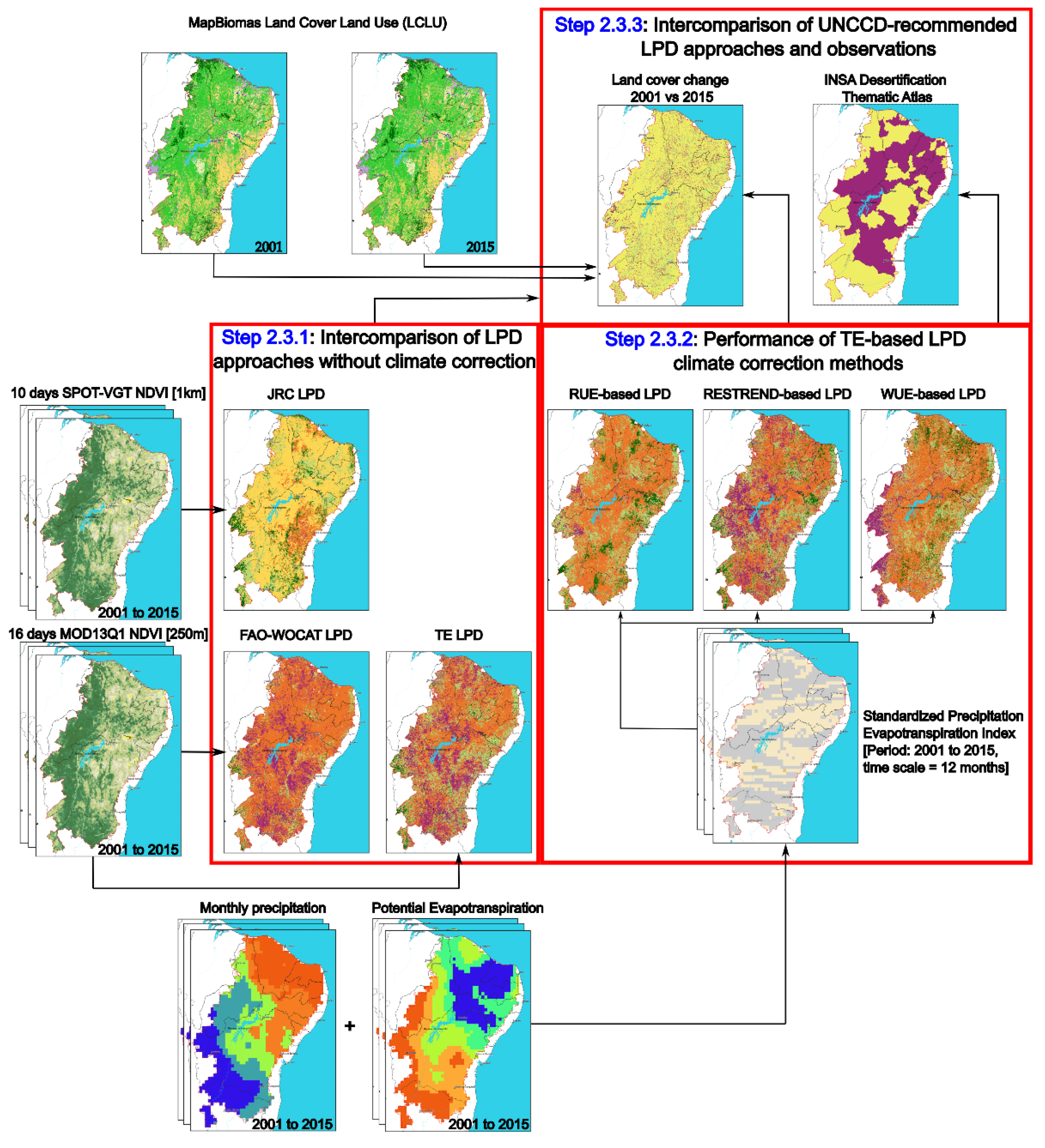
The desertification thematic atlas provided by the National Semiarid Institute (INSA) was used to validate degraded land in the BSR [62]. INSA follows a rigorous on-site quality control process before publishing reports, making them reliable benchmarks for assessing the performance of the three LPD approaches in capturing land degradation [63,64].

2.3. Methodology

The study period was from 2001 to 2015. The beginning year, 2001, was chosen because the MOD13Q1 and MOD16A2 products provide NDVI and ET time series from 2001 onwards. The final year, 2015, was determined based on the absence of records in the PET dataset by Xavier et al. [53] (the base for deriving SPEI12); beyond this point, as well as the establishment of this year as the endpoint for the baseline assessment. The present study follows a set of general procedures, which are summarized in a workflow depicted in Figure 2. Each methodological step is explained and discussed in detail in the following subsections.

2.3.1. Intercomparison of LPD Approaches without Climate Correction

We aligned the LPD data from the TE, JRC, and FAO-WOCAT at the pixel scale and then classified the LPD pixels based on their observed annual precipitation rates. LPD data was obtained from the Trends.Earth tool [65]. Pixels with rates below the 25th percentile, between the 25th and 75th percentiles, and above the 75th percentile were assigned to low, moderate, and high precipitation zones, respectively. This classification allowed us to analyze the performance of the LPD approaches in different precipitation regimes. After this, we then conducted a pixel-to-pixel evaluation using a categorical statistic (see below) to quantify the similarity between the three LPD approaches for each precipitation regime. For simplicity, the LPD pixels with declining values were classified as degraded land, and those with moderate decline, stressed, stable, and increasing values as non-degraded land. We applied stratified sampling with three strata (low, moderate, and high precipitation) to ensure representativeness and balance. We randomly selected 10,000 pixels per stratum (benchmark pixels). This task was performed using the sampling R package version 2.90 [66].
The similarity statistic (S) is based on a contingency table with two categories: degraded land and non-degraded land (Table 2). The table contains four cells denoted by labels “a” and “d” for LPD estimates that coincide and labels “b” and “c” for estimates that do not coincide in terms of pixel count.
Equation (1) computes the similarity statistic (S), which quantifies the proportion of coincident classes derived from LPD products on a scale from 0 to 1, where 1 denotes a perfect score.
S = a + d a + b + c + d
The formulation of the S statistic is similar to the accuracy metric employed for assessing binary class maps using in situ observations [67]. However, in the comparison of the two LPD rasters presented in Table 2, we do not treat either as the ground truth. Consequently, we propose to use the S statistic to avoid confusion.

2.3.2. Performance of TE-Based LPD Climate Correction Methods

The SPEI12 time series for December 2001 to December 2015 was used to identify meteorological drought in the BSR. This time scale captures long-term extreme drought conditions and has been used in previous studies to evaluate the impact of drought on vegetation and land productivity. This study defines a dry spell as at least two consecutive months with SPEI12 below −1.00 and ends when SPEI12 rises above −1.00. Four drought intensity classes were identified: mild (−1 to 0), moderate (−1.5 to −1), severe (−2 to −1.5), and extreme (≤−2). The area affected by drought was measured by counting pixels and grouping them by drought class and month. The long-term drought severity per pixel was calculated by summing negative SPEI12 values and converting them to an absolute value. Drought severity rasters were resampled to match their spatial resolution with the LPD raster (i.e., RUE, RESTREND, and WUE) using bilinear interpolation and scaled from 0 to 1, with 0 representing the lowest severity and 1 the highest.
For simplicity, LPD pixels with declining values were classified as degraded land and those with other categories as non-degraded land. Stratified sampling with two strata (i.e., degraded and non-degraded land) was used with a sample size of 10,000 pixels per stratum to ensure representativeness and balance. The nonparametric Kruskal–Wallis and Dunn’s tests were conducted to determine whether significant drought severity differences exist between degraded and non-degraded pixels. The Bonferroni-adjusted p-value threshold for statistical significance was set at 0.05. These nonparametric tests, chosen due to the lack of normality assumption in the stratified data [68,69], were implemented using the R package stats (version 4.1.2) [70]. This protocol was applied to the TE-based LPD raster without climate correction to evaluate the effect of climate correction on the detection of land degradation under drought conditions.

2.3.3. Intercomparison of UNCCD-Recommended LPD Approaches and Observations

We evaluated the accuracy of LPD approaches in detecting land degradation, with and without climate correction. We used benchmark pixels from the INSA’s desertification cores and the degraded pixels identified by the MapBiomas project (2001–2015) [55]. To minimize bias, we randomly selected 10,000 pixels classified as degraded from INSA and MapBiomas for each approach, including TE, JRC-LPD, FAO-WOCAT, RUE-based LPD, RE-STREND-based LPD, and WUE-based LPD. Next, we performed a pixel-by-pixel comparison between the INSA map and the MapBiomas project and calculated the hit rate by assessing the fraction of degraded pixels that were correctly classified as degraded by each method (Table 3). We repeated this process six times to determine the mean accuracy and corresponding standard deviation.
The hit rate (Hr) is based on the confusion matrix shown in Table 3. The table contains the number of true positives (TP), false positives (FP), true negatives (TN), and false negatives (FN). The hit rate, also referred to as recall or sensitivity, measures the LPD approach’s ability to identify actual positive cases (TP and FN) as positive (TP) [71]. This metric is also known as recall or sensitivity. A high Hr score signifies that the LPD approach correctly identifies a significant proportion of degraded pixels, while a low Hr score suggests that the approach fails to identify many degraded land cases.
Equation (2) computes the Hr, where 1 denotes a perfect score.
H r = T P T P + F N

3. Results

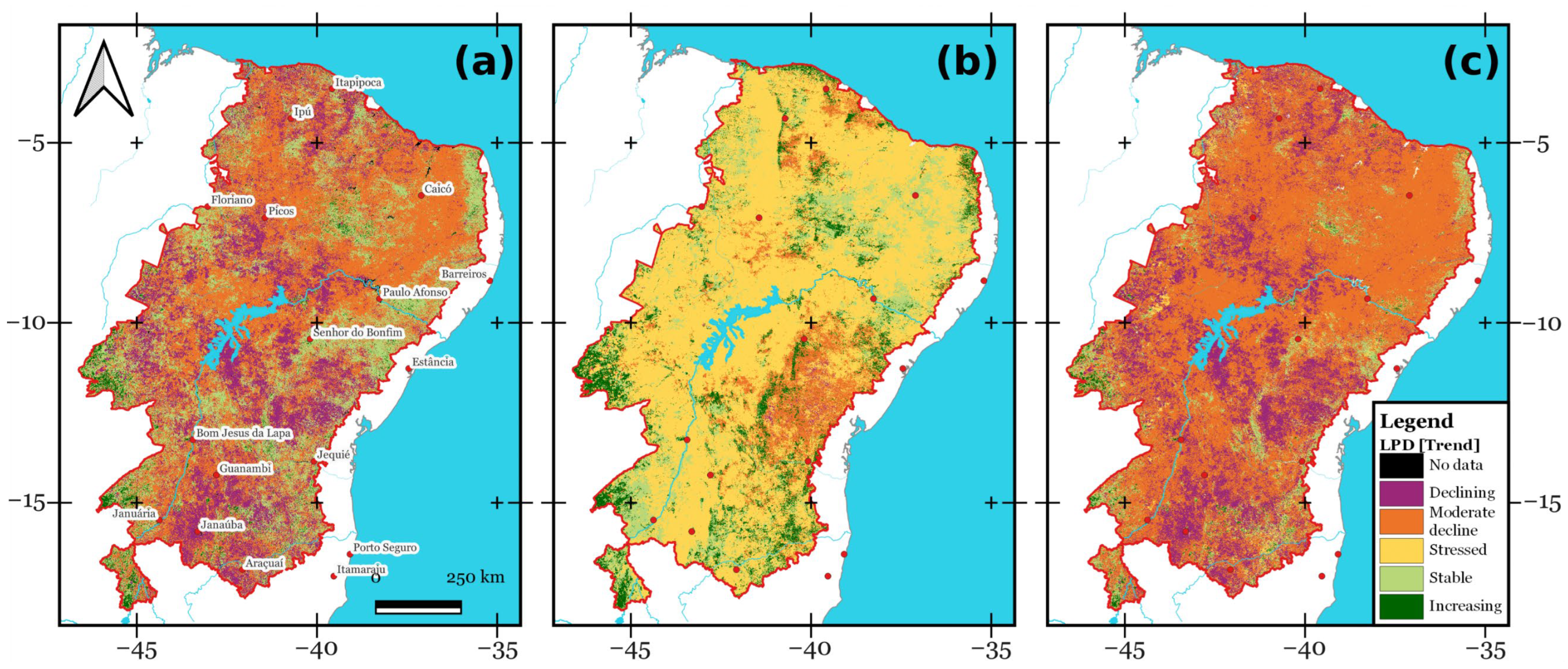
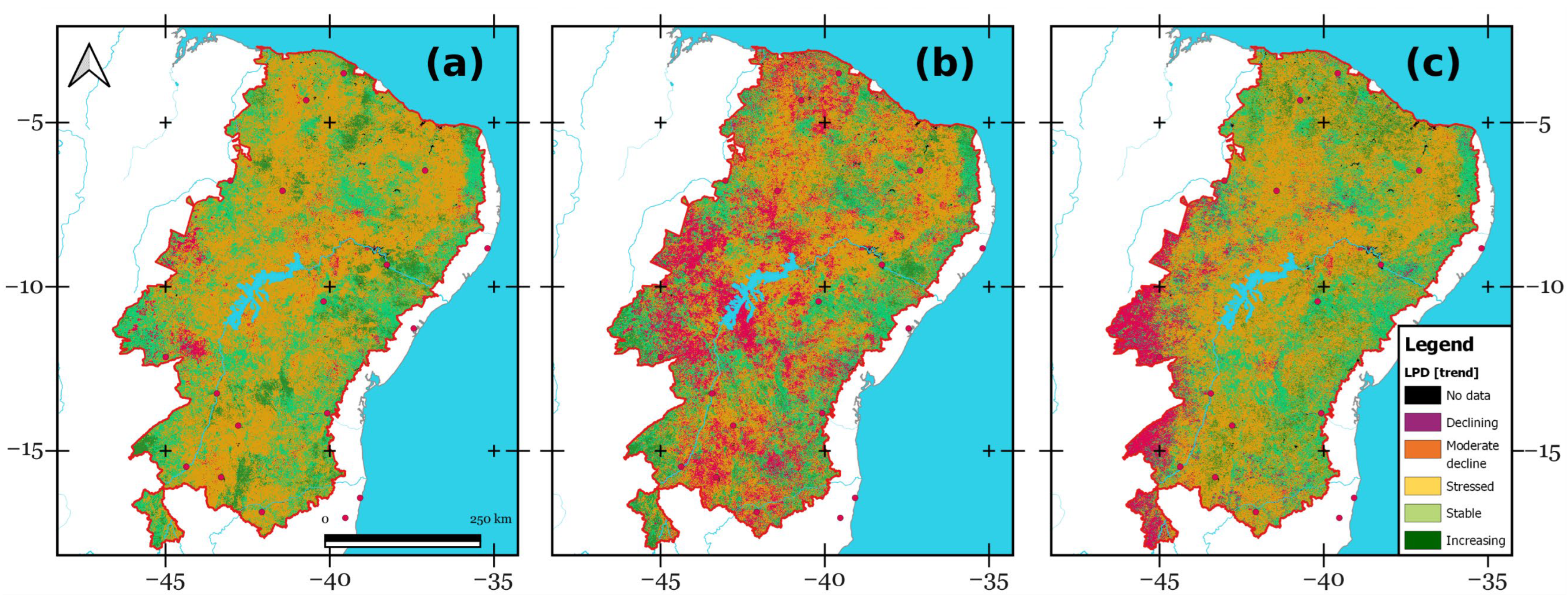
3.1. Intercomparison between LPD from the TE, JRC-LPD, and FAO-WOCAT Approaches

Figure 3 compares the land productivity of the three approaches over a study area from 2001 to 2015. Figure 3b depicts the land degradation derived from JRC-LPD. The JRC-LPD approach indicates less degraded land (i.e., declining = 4242 km2, moderate decline = 111,139 km2; stressed = 744,844 km2) compared to TE (i.e., declining = 248,075 km2, moderate decline = 545,985 km2; stressed = 1787 km2) and FAO-WOCAT (i.e., declining = 246,783 km2, moderate decline = 733,946 km2; stressed = 33,705 km2). The three approaches show the highest concentration of declining land in the Bahia state (JRC-LPD = 3846 km2, FAO-WOCAT = 118,445 km2, and TE = 117,424 km2). While variations in the extent of degraded land exist, the JRC-LPD approach identified Rio Grande do Norte state as possessing the lowest quantity of degraded land (5.88 km2). Conversely, the FAO-WOCAT and TE approaches identified the Alagoas state as having the smallest amount of degraded land, with respective estimates of 312 km2 and 322 km2.
Figure 4 displays the regions with a decrease in dynamic land productivity (i.e., degraded land). The spatial patterns of degraded lands, as estimated by the FAO-WOCAT and TE approaches, are similar.
We assessed the association between the distribution of degraded land and annual precipitation patterns. This assessment involved analyzing the similarity (Equation (1)) between the outputs presented in Figure 4 for each approach, considering a random selection of 10,000 pixels with low, moderate, and high precipitation regimes, respectively. Table 4 shows that the similarities among the three maps are higher under moderate and high precipitation regimes compared to the Low precipitation regime. The highest similarity across all precipitation regimes is found between TE and FAO-WOCAT, with values of 0.956, 0.971, and 0.972 for low, moderate, and high precipitation levels, respectively. The JRC-LPD map shows relatively lower similarity values when compared to TE and FAO-WOCAT, ranging from 0.748 to 0.814.
We used the Kruskal–Wallis’s rank sum and Dunn’s tests to identify statistical differences in similarity for the precipitation regime. We found no significant difference in the distribution of the similarity across the three levels of precipitation regime (i.e., low, moderate, and high) at a significance level of 0.05 (p-value = 0.094). These findings suggest that the TE and FAO-WOCAT provide more consistent representations of spatial patterns of degraded lands in the BSR (Figure 4). However, we did not find evidence indicating that the precipitation regime affects the similarity between these approaches (Table 4).

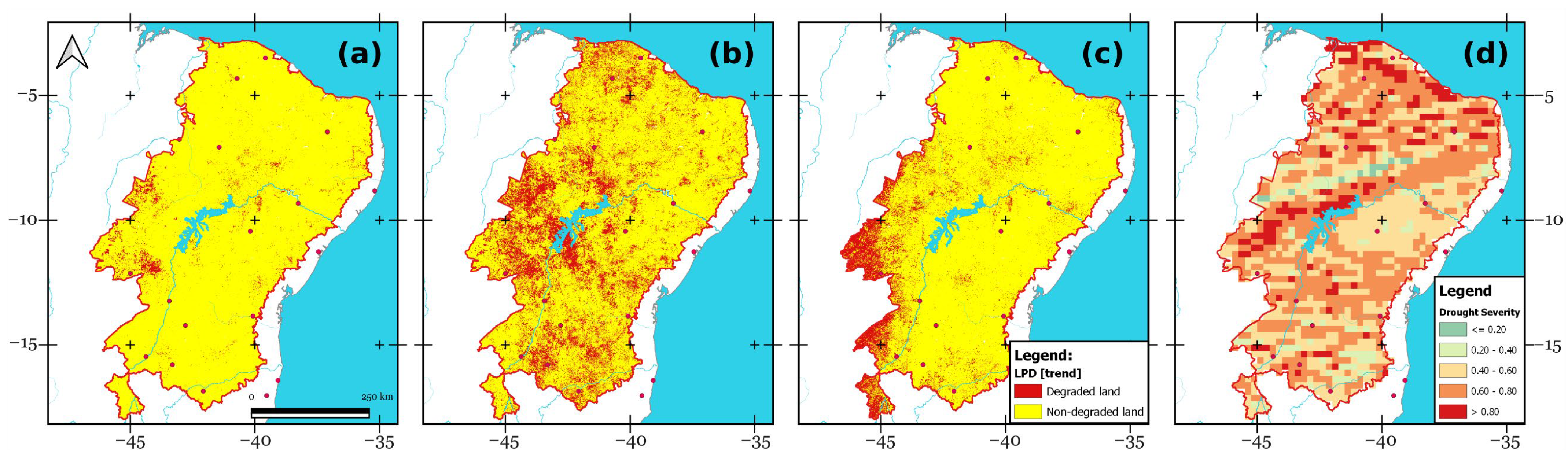
3.2. Performance of TE-Based LPD Climate Correction Methods in Drought-Prone Subregions

The UNCCD endorses the implementation of a climate-based adjustment in regions where precipitation may impact the LPD [72]. To date, this climate correction is only available via the Trends.Earth tool for the TE approach. When applied to the TE output (Figure 3a), three maps are possible (Figure 5), depending on the chosen climatic correction (i.e., RUE-based LPD, RESTREND-based LPD, and WUE-based LPD).
Figure 5 depicts a comparative analysis of land productivity over a study area from 2001 to 2015, as assessed by the RUE-based LPD, RESTREND-based LPD, and WUE-based LPD methods. All three approaches show a smaller area of degraded land than that exhibited by the non-corrected TE version (i.e., declining productivity = 248,075 km2). The LPD approach based on RUE estimates 29,519 km2, 635,289 km2, and 1661 km2 of declining, moderate decline, and stressed land, respectively. The RESTREND-based LPD approach estimates 213,248 km2, 490,643 km2, and 1634 km2 of declining, moderate decline, and stressed land, respectively. The WUE-based LPD approach estimates 85,125 km2, 584,640 km2, and 1263 km2 of declining, moderate decline, and stressed land, respectively. Overall, the application of the RUE-based LPD approach demonstrates a minimal extent of degraded land, primarily located in the central-west region of the study area. In contrast, the implementation of the RESTREND-based LPD methodology reveals a significant amount of degraded land, concentrated predominantly in the central, southern, and western sections of the Sertão.
It is noteworthy that the state of Bahia exhibits the highest concentration of declining land productivity in all three approaches. The state of Maranhão displays the smallest extent of degraded land as per the WUE-based LPD method and the state of Alagoas for the RESTREND-based LPD and RUE-based LPD methods (Figure 6a–c).
In scientific literature, drought is recognized as a crucial factor that drives land degradation in regions with arid and semiarid climates [63,73]. The Sertão region frequently experiences drought [11,14] (Figure 6d), which can occur in any location in the NEB, regardless of the annual rainfall patterns [74].
We assessed drought severity on randomly selected control pixels to investigate the impact of droughts on the detection of degraded lands. We categorized these pixels as either degraded or non-degraded (i.e., Figure 6a–c) within each TE-based LPD climate correction method (i.e., RUE-based LPD, RESTREND-based LPD, and WUE-based LPD). We employed the Kruskal–Wallis rank sum and Dunn’s tests to identify statistical differences in drought severity for each climate correction method [75]. Our findings revealed evidence of a difference in drought severity between degraded land and non-degraded land groups for RUE-based LPD (p-value < 0.01) and WUE-based LPD (p-value = 0.011), but not for RESTREND-based LPD (p-value = 0.518) at a significance level of 0.05. The pixels classified as degraded by the RUE and WUE methods showed a lower level of drought severity than their non-degraded counterparts.
The findings indicate that both the RUE and WUE climate corrections tend to categorize pixels subjected to less severe dry spells as degraded, while areas exposed to more severe droughts are classified as non-degraded. However, these outcomes may not correctly represent the identification of truly degraded lands. In the following section, we assess the performance of the three climate-corrected TE LPDs in identifying degraded lands by comparing them to maps of degraded lands generated by the MapBiomas project and the INSA’s degraded land atlas. The MapBiomas initiative employs Landsat imagery at a spatial resolution of 30 m, supported by ground validation points and sophisticated classification algorithms [55]. In contrast, the INSA relies on on-site inspections to detect the occurrence of degraded zones.

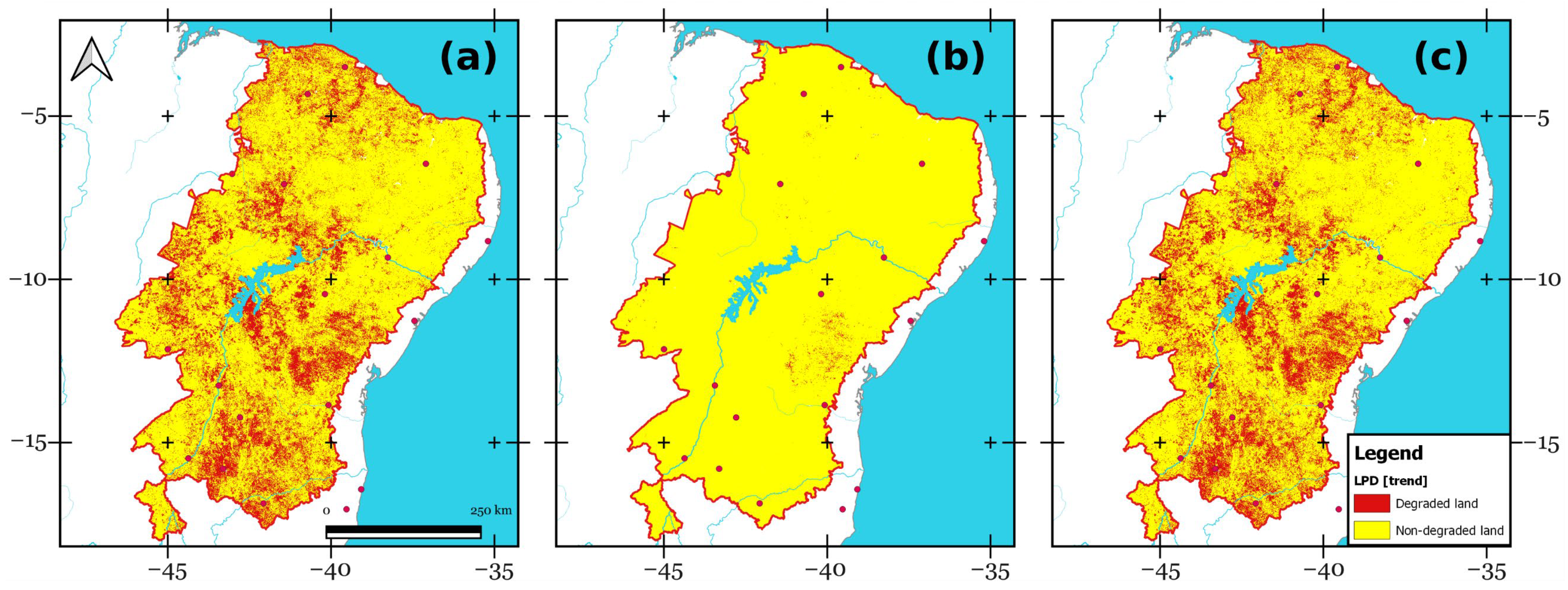
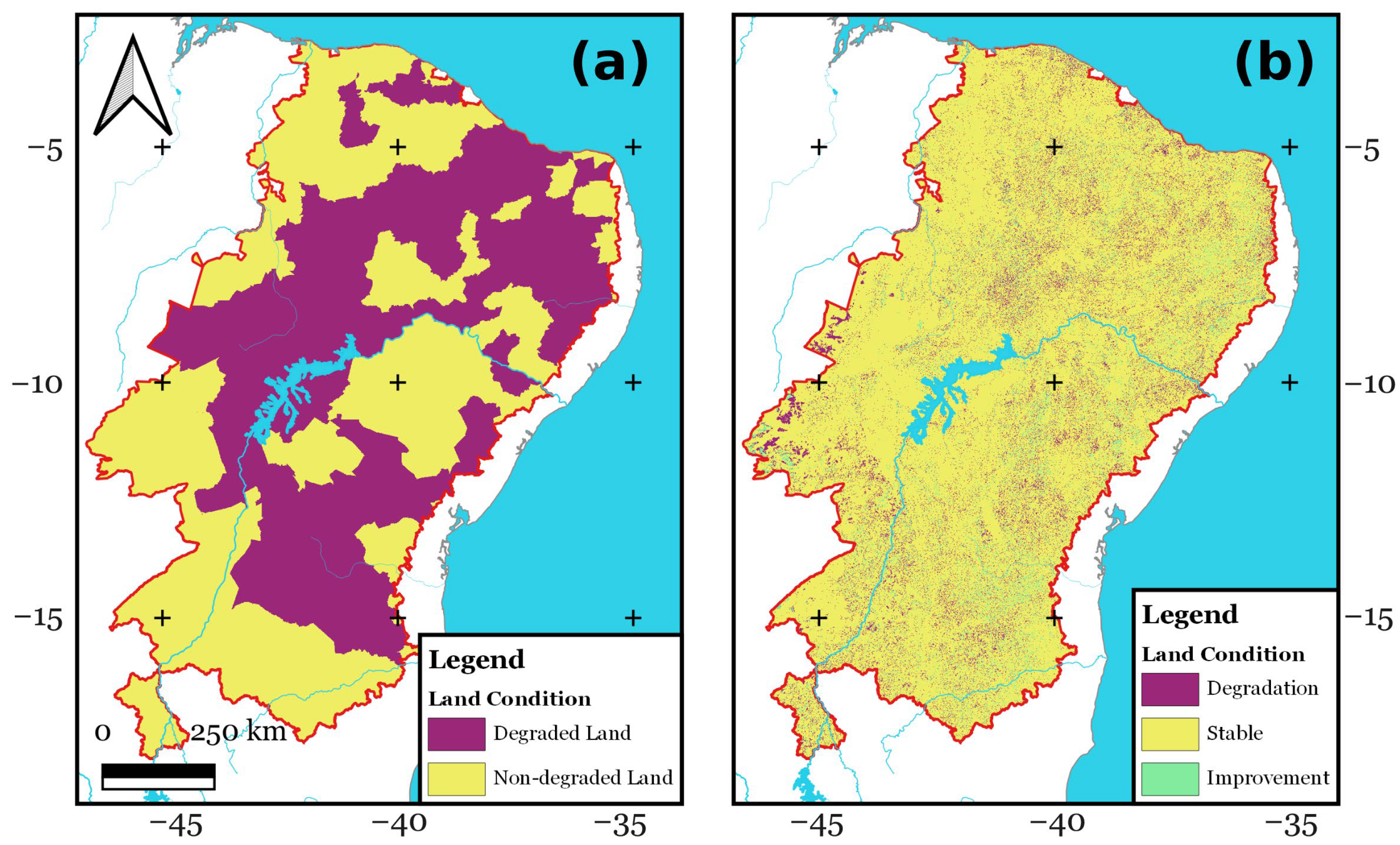
3.3. Accuracy of the UNCCD-Recommended LPD Approaches

By utilizing Equation (2), we compared the binary maps in Figure 4a–c and Figure 6a–c, and the maps of degraded lands reported by MapBiomas and INSA (Figure 7) to evaluate the hit rate of JRC-LPD, FAO-WOCAT, RUE-based LPD, RESTREND-based LPD, and WUE-based LPD for identifying degraded land areas.
Table 5 demonstrates that among the six methods, FAO-WOCAT and RESTREND exhibit the highest hit rate scores when assessed against INSA (0.219 and 0.224, respectively) and MapBiomas (0.401 and 0.394, respectively). In contrast, JRC presents the lowest hit rate scores in comparison to both benchmarks, with 0.005 for INSA and 0.008 for MapBiomas. The hit rate scores of all methods are better when evaluated against MapBiomas rather than INSA, suggesting that they are relatively more accurate in relation to MapBiomas.

4. Discussion

In this study, we attempt to fill the knowledge gap by comparing different methods recommended by the UNCCD to evaluate trends in land productivity. We also explored how well these methods can detect land degradation and how the detectability of land degradation is related to precipitation patterns and long-term drought severity in the BSR.
The TE and FAO-WOCAT approaches identify a similar spatial pattern of degraded land, with a more extensive area identified in comparison to the JRC-LPD method (Figure 3). The application of annual mean NDVI values derived from MOD13Q1 as a reference variable in TE and FAO-WOCAT is probably a contributing factor to this similarity [35]. The argument gains strength if one considers that FAO-WOCAT is a simplified version of the JRC-LPD approach that integrates different elements of the TE approach [34,35,36]. An additional factor contributing to the discrepancies in the spatial distribution of degraded lands between JRC-LPD and TE/FAO-WOCAT (Figure 4) can be attributed to the differences in spatial resolution of the NDVI data sources. JRC-LPD employs NDVI scenes with a 1 km spatial resolution, whereas TE and FAO-WOCAT utilize NDVI images at 250 m (Table 1). Addressing this challenge, Giulani et al. [65] showed that employing Earth observation-based products with coarse spatial resolution in land degradation assessments poses a limitation, as it leads to an insufficient representation of localized degradation processes.
A comparison of Figure 1b and Figure 4 and Table 4 reveals that the three methods (i.e., TE, JRC-LPD, and FAO-WOCAT) yield similar outcomes in Sertão regions characterized by higher annual precipitation levels. The similarity among the three approaches, where annual precipitation is greater, can be partially attributed to the reduced NDVI fluctuations over the course of the year in contrast to areas with less precipitation [25]. Nevertheless, there is not enough evidence to demonstrate that the precipitation patterns significantly impact the spatial distribution of degraded lands as identified by these methods (Table 4).
The RUE-based LPD, RESTREND-based LPD, and WUE-based LPD approaches incorporate climatic correction methods to improve the identification of degraded lands by eliminating the influence of rainfall variability on the annualized NDVI signal [27]. As expected, the implementation of this correction results in the delineation of degraded areas with a reduced spatial extent (Figure 6), in comparison to the version without climate correction (Figure 3a). However, it is crucial to recognize that droughts recurrently impact the BSR, resulting in accelerated soil erosion, land degradation, and desertification due to the associated losses in vegetation cover [76]. Moreover, droughts frequently lead to widespread fires, causing considerable damage on the land [77]. The recovery of the land to its original state can take a long time [42]. Various land use and management regimes coexist in the drier parts of the Sertão, each exhibiting distinct NDVI response patterns in response to land management practices and environmental stressors [78]. Native vegetation, grasslands, and rainfed crops display a more rapid reaction to changes in precipitation but experience a slower recovery following prolonged drought events [37].
Our results reveal that areas identified as degraded by climate-corrected LPD methods exhibit lower drought severity compared to non-degraded areas, which is surprising and counterintuitive (Figure 6). For instance, RESTREND displays an unexpected characteristic, as it demonstrates no significant statistical difference in drought severity between degraded and non-degraded pixels. Previous studies have established that droughts substantially affect NEB vegetation, particularly grassland, scrubland, and rainfed crop areas [79,80]. Consequently, one would expect a correlation between degraded pixels and elevated levels of drought severity. However, such a correlation was not observed. Undoubtedly, the climate-based adjustment of the LPD tends to mask the influence of droughts on vegetation in the BSR, thus hiding the land degradation processes triggered by this climatic hazard. This specific characteristic is not unique to the BSR. It has also been observed in other semiarid regions [81]. Consequently, researchers have been motivated to adopt alternative methodologies in arid and semiarid areas [82]. An alternative methodology to address this limitation is to adopt the time series segmentation and residual trend analysis (TSS-RESTREND), which combines the advantages of the RESTREND and breaks for additive season and trend (BFAST) breakpoint detection methods [83].
While comparing observational data for assessments, we discovered that the LPD approach, utilizing RESTREND as a basis, and subsequently FAO-WOCAT and TE, provides the most accurate representation of degraded lands as identified by both the INSA thematic atlas and MapBiomas initiatives (Table 5). The RESTREND-based LPD approach is a statistical technique that detects long-term trends in time series data by fitting a linear model to the data and then analyzing the residuals (i.e., the differences between the observed values and the values predicted by the model). By focusing on the residuals, RESTREND can identify changes in the NDVI that are not explained by short-term or seasonal variations [41,84].
In land degradation assessment, low hit rates can result in the underestimation of degraded land, leading to incorrect policy decisions and ineffective management practices. Table 4 indicates that the hit rates of RESTREND, FAO-WOCAT, and TE are moderately low, which suggests that they frequently misclassify degraded land as non-degraded land. Our results also reveal a slight difference in hit rates between these approaches, indicating that incorporating climate correction results in only a marginal improvement in identifying degraded land.
Overall, the LPD approaches—RESTREND, TE, and FAO-WOCAT—provide the most accurate representation of LPD. However, users should exercise caution when using them due to their low hit rate (approximately 0.30). Further exploration of alternative algorithms and satellite-derived indices that more effectively capture the LPD for various land covers in the BSR and comparable semiarid regions is necessary. These results underscore the importance of validating degraded land maps generated by these methods (Figure 3 and Figure 5) at the local level before implementing interventions, thereby ensuring evidence-based decision-making.

5. Conclusions

The Brazilian Sertão region (BSR) is a well-known area affected by drought and land degradation. This study employed a three-step methodological framework to assess the performance of UNCCD-recommended LPD approaches in detecting degraded lands within the BSR. Our findings reveal that the TE and FAO-WOCAT approaches exhibit a similar spatial pattern of degraded land, identifying a larger area compared to the JRC-LPD method. While these approaches yield comparable results in regions with higher annual precipitation, no strong evidence demonstrates a significant impact of precipitation patterns on the spatial distribution of degraded lands.
Moreover, climate-corrected LPD methods (i.e., RUE, RESTREND, and WUE) tend to identify areas under lower drought severities as degraded, which contradicts previous research within the BSR. Among the climate-corrected LPD approaches, RESTREND, followed by FAO-WOCAT and TE, provides the best representation of degraded lands as indicated by benchmark data (i.e., INSA and MapBiomas). However, these methods exhibit low hit rates, potentially leading to the underestimation of degraded land and, consequently, incorrect policy decisions and suboptimal management practices.
In light of these findings, we recommend the further exploration of alternative algorithms and satellite-derived indices capable of effectively capturing LPD for diverse land covers in the BSR and other semiarid regions. Such advancements will improve land degradation monitoring, facilitating informed policy-making and management strategies to address land degradation in semiarid areas.

Author Contributions

Experiment design, F.P.-T., H.A.B., T.V.L.K. and G.A.D.; experimentation, I.T.; data analysis, C.L.G. and C.d.O.B.; writing, F.P.-T., H.A.B., G.A.D. and I.T. All authors have read and agreed to the published version of the manuscript.

Funding

This study was undertaken as part of the Satellite Desertification Monitoring Program in the Brazilian Semiarid Region [Grant Number 403223/2021-0] supported by the CNPq. It also had the support of Capes through Notice no. 28/2022—PDPG Social Vulnerability & Human Rights [Grant Number 88881.705050/2022-01].

Data Availability Statement

The TE, JRC-LPD, and FAO-WOCAT datasets in GeoTiff format covering the Sertão region, as illustrated in Figure 3, along with the RUE-based LPD, RESTREND-based LPD, and WUE-based LPD files in GeoTiff format depicted in Figure 5, can be found online at https://zenodo.org/record/7815318 (accessed on 23 February 2023). The MapBiomas Land Cover Land Use (LCLU) Collection 7 dataset used in this research is openly accessible at https://mapbiomas.org/en (accessed on 23 February 2023). The Thematic Atlas of Desertification, produced by the National Semiarid Institute (INSA) and employed in this study, is available to the public via reference [62]. The Standardized Precipitation Evapotranspiration Index (SPEI) analysis is performed using the gridded P and PET database developed by Xavier et al. [53].

Acknowledgments

The authors thank the anonymous reviewers and editor for their valuable feedback and recommendations.

Conflicts of Interest

The authors declare no conflict of interest.

References

  1. Wilhite, D.A.; Pulwarty, R.S. Drought and Water Crises, 2nd ed.; Wilhite, D., Pulwarty, R.S., Eds.; CRC Press: Boca Raton, FL, USA, 2018. [Google Scholar]
  2. McCabe, G.J.; Wolock, D.M. Variability and Trends in Global Drought. Earth Space Sci. 2015, 2, 223–228. [Google Scholar] [CrossRef]
  3. Moravec, V.; Markonis, Y.; Rakovec, O.; Svoboda, M.; Trnka, M.; Kumar, R.; Hanel, M. Europe under Multi-Year Droughts: How Severe Was the 2014–2018 Drought Period? Environ. Res. Lett. 2021, 16, 034062. [Google Scholar] [CrossRef]
  4. Apurv, T.; Cai, X. Regional Drought Risk in the Contiguous United States. Geophys. Res. Lett. 2021, 48, e2020GL092200. [Google Scholar] [CrossRef]
  5. Erfanian, A.; Wang, G.; Fomenko, L. Unprecedented Drought over Tropical South America in 2016: Significantly under-Predicted by Tropical SST. Sci. Rep. 2017, 7, 5811. [Google Scholar] [CrossRef]
  6. Jimenez, J.C.; Marengo, J.A.; Alves, L.M.; Sulca, J.C.; Takahashi, K.; Ferrett, S.; Collins, M. The Role of ENSO Flavours and TNA on Recent Droughts over Amazon Forests and the Northeast Brazil Region. Int. J. Climatol. 2021, 41, 3761–3780. [Google Scholar] [CrossRef]
  7. Cuartas, L.A.; do Amaral Cunha, A.P.M.; Alves, J.A.; Parra, L.M.P.; Deusdará-Leal, K.R.; Costa, L.C.M.; Molina, R.; Amore, D.; Broedel, E.; Seluchi, M.E.; et al. Recent Hydrological Droughts in Brazil and Their Impact on Hydropower Generation. Water 2022, 14, 601. [Google Scholar] [CrossRef]
  8. Gutiérrez, A.P.A.; Engle, N.L.; De Nys, E.; Molejón, C.; Martins, E.S. Drought Preparedness in Brazil. Weather Clim. Extrem. 2014, 3, 95–106. [Google Scholar] [CrossRef]
  9. Cunha, A.P.M.A.; Zeri, M.; Leal, K.D.; Costa, L.; Cuartas, L.A.; Marengo, J.A.; Tomasella, J.; Vieira, R.M.; Barbosa, A.A.; Cunningham, C.; et al. Extreme Drought Events over Brazil from 2011 to 2019. Atmosphere 2019, 10, 642. [Google Scholar] [CrossRef]
  10. Marengo, J.A.; Bernasconi, M. Regional Differences in Aridity/Drought Conditions over Northeast Brazil: Present State and Future Projections. Clim. Change 2015, 129, 103–115. [Google Scholar] [CrossRef]
  11. Marengo, J.A.; Torres, R.R.; Alves, L.M. Drought in Northeast Brazil—Past, Present, and Future. Theor. Appl. Climatol. 2017, 129, 1189–1200. [Google Scholar] [CrossRef]
  12. Marengo, J.A.; Alves, L.M.; Alvala, R.C.; Cunha, A.P.; Brito, S.; Moraes, O.L.L. Climatic Characteristics of the 2010–2016 Drought in the Semiarid Northeast Brazil Region. An. Acad. Bras. Cienc. 2018, 90, 1973–1985. [Google Scholar] [CrossRef]
  13. Rossato, L.; dos Alvalá, R.C.S.; Marengo, J.A.; Zeri, M.; do Cunha, A.P.M.A.; Pires, L.B.M.; Barbosa, H.A. Impact of Soil Moisture on Crop Yields over Brazilian Semiarid. Front. Environ. Sci. 2017, 5, 73. [Google Scholar] [CrossRef]
  14. Brito, S.S.B.; Cunha, A.P.M.A.; Cunningham, C.C.; Alvalá, R.C.; Marengo, J.A.; Carvalho, M.A. Frequency, Duration and Severity of Drought in the Semiarid Northeast Brazil Region. Int. J. Climatol. 2018, 38, 517–529. [Google Scholar] [CrossRef]
  15. Spera, S.A.; Galford, G.L.; Coe, M.T.; Macedo, M.N.; Mustard, J.F. Land-Use Change Affects Water Recycling in Brazil’s Last Agricultural Frontier. Global Change Biol. 2016, 22, 3405–3413. [Google Scholar] [CrossRef] [PubMed]
  16. Marengo, J.A.; Galdos, M.V.; Challinor, A.; Cunha, A.P.; Marin, F.R.; dos Vianna, M.S.; Alvala, R.C.S.; Alves, L.M.; Moraes, O.L.; Bender, F. Drought in Northeast Brazil: A Review of Agricultural and Policy Adaptation Options for Food Security. Clim. Resil. Sustain. 2022, 1, e17. [Google Scholar] [CrossRef]
  17. Hayes, M.; Svoboda, M.; Wall, N.; Widhalm, M. The Lincoln Declaration on Drought Indices: Universal Meteorological Drought Index Recommended. Bull. Am. Meteorol. Soc. 2011, 92, 485–488. [Google Scholar] [CrossRef]
  18. Campos, J.; Carvalho, T. Drought and Water Policies in Northeast Brazil: Backgrounds and Rationale. Water Policy 2008, 10, 425–438. [Google Scholar] [CrossRef]
  19. Mishra, A.K.; Singh, V.P. A Review of Drought Concepts. J. Hydrol. 2010, 391, 202–216. [Google Scholar] [CrossRef]
  20. De Assis Souza Filho, F.; Formiga-Johnsson, R.M.; de Carvalho Studart, T.M.; Abicalil, M.T. From Drought to Water Security: Brazilian Experiences and Challenges. In Global Water Security; Springer: Berlin/Heidelberg, Germany, 2018; pp. 233–265. [Google Scholar]
  21. Park, S.-Y.; Sur, C.; Kim, J.-S.; Lee, J.-H. Evaluation of Multi-Sensor Satellite Data for Monitoring Different Drought Impacts. Stoch. Environ. Res. Risk Assess. 2018, 32, 2551–2563. [Google Scholar] [CrossRef]
  22. Paredes-Trejo, F.; Barbosa, H.A.; Giovannettone, J.; Kumar, T.V.L.; Thakur, M.K.; de Buriti, C.O.; Uzcátegui-Briceño, C. Drought Assessment in the São Francisco River Basin Using Satellite-Based and Ground-Based Indices. Remote Sens. 2021, 13, 3921. [Google Scholar] [CrossRef]
  23. Stanturf, J.A. Landscape Degradation and Restoration. In Soils and Landscape Restoration; Elsevier: Amsterdam, The Netherlands, 2021; pp. 125–159. [Google Scholar]
  24. Nachtergaele, F.O.F.; Licona-Manzur, C. The Land Degradation Assessment in Drylands (LADA) Project: Reflections on Indicators for Land Degradation Assessment. In The Future of Drylands; Springer: Dordrecht, The Netherlands, 2008; pp. 327–348. [Google Scholar]
  25. Barbosa, H.A.; Huete, A.R.; Baethgen, W.E. A 20-Year Study of NDVI Variability over the Northeast Region of Brazil. J. Arid Environ. 2006, 67, 288–307. [Google Scholar] [CrossRef]
  26. Grainger, A. Is Land Degradation Neutrality Feasible in Dry Areas? J. Arid Environ. 2015, 112, 14–24. [Google Scholar] [CrossRef]
  27. Sims, N.C.; England, J.R.; Newnham, G.J.; Alexander, S.; Green, C.; Minelli, S.; Held, A. Developing Good Practice Guidance for Estimating Land Degradation in the Context of the United Nations Sustainable Development Goals. Environ. Sci. Policy 2019, 92, 349–355. [Google Scholar] [CrossRef]
  28. Diallo, H.A. United Nations Convention to Combat Desertification (UNCCD). In The Future of Drylands; Springer: Dordrecht, The Netherlands, 2008; pp. 13–16. [Google Scholar]
  29. Sims, N.C.; Barger, N.N.; Metternicht, G.I.; England, J.R. A Land Degradation Interpretation Matrix for Reporting on UN SDG Indicator 15.3.1 and Land Degradation Neutrality. Environ. Sci. Policy 2020, 114, 1–6. [Google Scholar] [CrossRef]
  30. Akhtar-Schuster, M.; Stringer, L.C.; Erlewein, A.; Metternicht, G.; Minelli, S.; Safriel, U.; Sommer, S. Unpacking the Concept of Land Degradation Neutrality and Addressing Its Operation through the Rio Conventions. J. Environ. Manag. 2017, 195, 4–15. [Google Scholar] [CrossRef]
  31. Paredes-Trejo, F.; Barbosa, H.; Giovannettone, J.; Kumar, T.V.L.; Thakur, M.K.; de Oliveira Buriti, C. Drought Variability and Land Degradation in the Amazon River Basin. Front. Earth Sci. 2022, 10, 1–16. [Google Scholar] [CrossRef]
  32. Barker, L.J.; Rickards, N.J.; Sarkar, S.; Hannaford, J.; King-Okumu, C.; Rees, G. Good Practice Guidance for National Reporting on UNCCD Strategic Objective 3: To Mitigate, Adapt to, and Manage the Effects of Drought in Order to Enhance Resilience of Vulnerable Populations and Ecosystems; United Nations Convention to Combat Desertification: New York, NY, USA, 2021. [Google Scholar]
  33. Guo, W.Q.; Yang, T.B.; Dai, J.G.; Shi, L.; Lu, Z.Y. Vegetation Cover Changes and Their Relationship to Climate Variation in the Source Region of the Yellow River, China, 1990–2000. Int. J. Remote Sens. 2008, 29, 2085–2103. [Google Scholar] [CrossRef]
  34. Rotllan-Puig, X.; Ivits, E.; Cherlet, M. LPDynR: A New Tool to Calculate the Land Productivity Dynamics Indicator. Ecol. Indic. 2021, 133, 108386. [Google Scholar] [CrossRef]
  35. Teich, I.; Roglich, M.G.; Corso, M.L.; García, C.L. Combining Earth Observations, Cloud Computing, and Expert Knowledge to Inform National Level Degradation Assessments in Support of the 2030 Development Agenda. Remote Sens. 2019, 11, 2918. [Google Scholar] [CrossRef]
  36. Food and Agriculture Organization. Overview of Land Degradation Neutrality (LDN) in Europe and Central Asia; FAO, Ed.; FAO: Roma, Italy, 2022. [Google Scholar]
  37. Barbosa, H.A.; Kumar, T.V.L. Influence of Rainfall Variability on the Vegetation Dynamics over Northeastern Brazil. J. Arid Environ. 2016, 124, 377–387. [Google Scholar] [CrossRef]
  38. De Oliveira, M.L.; dos Santos, C.A.C.; de Oliveira, G.; Silva, M.T.; da Silva, B.B.; de Cunha, J.E.B.L.; Ruhoff, A.; Santos, C.A.G. Remote Sensing-Based Assessment of Land Degradation and Drought Impacts over Terrestrial Ecosystems in Northeastern Brazil. Sci. Total Environ. 2022, 835, 155490. [Google Scholar] [CrossRef]
  39. Prince, S.D. Challenges for Remote Sensing of the Sustainable Development Goal SDG 15.3.1 Productivity Indicator. Remote Sens. Environ. 2019, 234, 111428. [Google Scholar] [CrossRef]
  40. Wessels, K.J.; Prince, S.D.; Malherbe, J.; Small, J.; Frost, P.E.; VanZyl, D. Can Human-Induced Land Degradation Be Distinguished from the Effects of Rainfall Variability? A Case Study in South Africa. J. Arid Environ. 2007, 68, 271–297. [Google Scholar] [CrossRef]
  41. Wessels, K.J.; van den Bergh, F.; Scholes, R.J. Limits to Detectability of Land Degradation by Trend Analysis of Vegetation Index Data. Remote Sens. Environ. 2012, 125, 10–22. [Google Scholar] [CrossRef]
  42. De Santiago, D.B.; Barbosa, H.A.; Filho, W.L.F.C.; de Oliveira-Júnior, J.F.; Paredes-Trejo, F.; de Oliveira Buriti, C. Variability of Water Use Efficiency Associated with Climate Change in the Extreme West of Bahia. Sustainability 2022, 14, 16004. [Google Scholar] [CrossRef]
  43. Markos, A.; Sims, N.; Giuliani, G. Beyond the SDG 15.3.1 Good Practice Guidance 1.0 Using the Google Earth Engine Platform: Developing a Self-Adjusting Algorithm to Detect Significant Changes in Water Use Efficiency and Net Primary Production. Big Earth Data 2023, 7, 59–80. [Google Scholar] [CrossRef]
  44. Noojipady, P.; Prince, S.D.; Rishmawi, K. Reductions in Productivity Due to Land Degradation in the Drylands of the Southwestern United States. Ecosyst. Health Sustain. 2015, 1, 1–15. [Google Scholar] [CrossRef]
  45. Jiang, L.; Bao, A.; Jiapaer, G.; Liu, R.; Yuan, Y.; Yu, T. Monitoring Land Degradation and Assessing Its Drivers to Support Sustainable Development Goal 15.3 in Central Asia. Sci. Total Environ. 2022, 807, 150868. [Google Scholar] [CrossRef]
  46. Giuliani, G.; Mazzetti, P.; Santoro, M.; Nativi, S.; Van Bemmelen, J.; Colangeli, G.; Lehmann, A. Knowledge Generation Using Satellite Earth Observations to Support Sustainable Development Goals (SDG): A Use Case on Land Degradation. Int. J. Appl. Earth Obs. Geoinf. 2020, 88, 102068. [Google Scholar] [CrossRef]
  47. Alamanos, A.; Linnane, S. Estimating SDG Indicators in Data-Scarce Areas: The Transition to the Use of New Technologies and Multidisciplinary Studies. Earth 2021, 2, 635–652. [Google Scholar] [CrossRef]
  48. Kang, W.; Wang, T.; Liu, S. The Response of Vegetation Phenology and Productivity to Drought in Semi-Arid Regions of Northern China. Remote Sens. 2018, 10, 727. [Google Scholar] [CrossRef]
  49. Vicente-Serrano, S.; Cabello, D.; Tomás-Burguera, M.; Martín-Hernández, N.; Beguería, S.; Azorin-Molina, C.; Kenawy, A. Drought Variability and Land Degradation in Semiarid Regions: Assessment Using Remote Sensing Data and Drought Indices (1982–2011). Remote Sens. 2015, 7, 4391–4423. [Google Scholar] [CrossRef]
  50. Tirivarombo, S.; Osupile, D.; Eliasson, P. Drought Monitoring and Analysis: Standardised Precipitation Evapotranspiration Index (SPEI) and Standardised Precipitation Index (SPI). Phys. Chem. Earth Parts A/B/C 2018, 106, 1–10. [Google Scholar] [CrossRef]
  51. Maia, A.G.; Cesano, D.; Miyamoto, B.C.B.; Eusebio, G.S.; de Silva, P.A.O. Climate Change and Farm-Level Adaptation: The Brazilian Sertão. Int. J. Clim. Change Strateg. Manag. 2018, 10, 729–751. [Google Scholar] [CrossRef]
  52. Pilz, T.; Delgado, J.M.; Voss, S.; Vormoor, K.; Francke, T.; Costa, A.C.; Martins, E.; Bronstert, A. Seasonal Drought Prediction for Semiarid Northeast Brazil; Institut für Erd-und Umweltwissenschaften: Potsdam, Germany, 2019. [Google Scholar]
  53. Xavier, A.C.; King, C.W.; Scanlon, B.R. Daily Gridded Meteorological Variables in Brazil (1980–2013). Int. J. Climatol. 2016, 36, 2644–2659. [Google Scholar] [CrossRef]
  54. Berry, P.A.M.; Garlick, J.D.; Smith, R.G. Near-Global Validation of the SRTM DEM Using Satellite Radar Altimetry. Remote Sens. Environ. 2007, 106, 17–27. [Google Scholar] [CrossRef]
  55. Souza, C.M.; Shimbo, J.Z.; Rosa, M.R.; Parente, L.L.; Alencar, A.A.; Rudorff, B.F.T.; Hasenack, H.; Matsumoto, M.; Ferreira, L.G.; Souza-Filho, P.W.M.; et al. Reconstructing Three Decades of Land Use and Land Cover Changes in Brazilian Biomes with Landsat Archive and Earth Engine. Remote Sens. 2020, 12, 2735. [Google Scholar] [CrossRef]
  56. Vicente-Serrano, S.M.; Beguería, S.; López-Moreno, J.I. A Multiscalar Drought Index Sensitive to Global Warming: The Standardized Precipitation Evapotranspiration Index. J. Clim. 2010, 23, 1696–1718. [Google Scholar] [CrossRef]
  57. Xavier, A.C. An Update of Xavier, King and Scanlon (2016) Daily Precipitation Gridded Data Set for the Brazil. In Proceedings of the 18th Brazilian Symposium on Remote Sensing, Santos, SP, Brazil, 28–31 May 2017; pp. 28–33. [Google Scholar]
  58. Beguería, S.; Vicente-Serrano, S.M.; Reig, F.; Latorre, B. Standardized Precipitation Evapotranspiration Index (SPEI) Revisited: Parameter Fitting, Evapotranspiration Models, Tools, Datasets and Drought Monitoring. Int. J. Climatol. 2014, 34, 3001–3023. [Google Scholar] [CrossRef]
  59. Neves, A.K.; Körting, T.S.; Fonseca, L.M.G.; Escada, M.I.S. Assessment of TerraClass and MapBiomas Data on Legend and Map Agreement for the Brazilian Amazon Biome. Acta Amaz. 2020, 50, 170–182. [Google Scholar] [CrossRef]
  60. Paredes-Trejo, F.; Barbosa, H.A.; Giovannettone, J.; Kumar, T.V.L.; de Oliveira Buriti, C.; Prieto, J. Assessing Satellite-Based Products in Characterizing Agricultural Drought Under Climate Change in Northeast Brazil. In Climate Change and Agriculture; Wiley: Hoboken, NJ, USA, 2022; pp. 426–442. [Google Scholar]
  61. Elnashar, A.; Wang, L.; Wu, B.; Zhu, W.; Zeng, H. Synthesis of Global Actual Evapotranspiration from 1982 to 2019. Earth Syst. Sci. Data 2021, 13, 447–480. [Google Scholar] [CrossRef]
  62. Santana, M.O. Atlas Das Áreas Susceptíveis à Desertificação Do Brasil; Ministry of Environment of Brazil: Brasília, Brazil, 2007.
  63. Da Vieira, R.M.S.P.; Sestini, M.F.; Tomasella, J.; Marchezini, V.; Pereira, G.R.; Barbosa, A.A.; Santos, F.C.; Rodriguez, D.A.; do Nascimento, F.R.; Santana, M.O.; et al. Characterizing Spatio-Temporal Patterns of Social Vulnerability to Droughts, Degradation and Desertification in the Brazilian Northeast. Environ. Sustain. Indic. 2020, 5, 100016. [Google Scholar] [CrossRef]
  64. Cunha, A.P.M.; Alvalá, R.C.; Nobre, C.A.; Carvalho, M.A. Monitoring Vegetative Drought Dynamics in the Brazilian Semiarid Region. Agric. For. Meteorol. 2015, 214–215, 494–505. [Google Scholar] [CrossRef]
  65. Giuliani, G.; Chatenoux, B.; Benvenuti, A.; Lacroix, P.; Santoro, M.; Mazzetti, P. Monitoring Land Degradation at National Level Using Satellite Earth Observation Time-Series Data to Support SDG15—Exploring the Potential of Data Cube. Big Earth Data 2020, 4, 3–22. [Google Scholar] [CrossRef]
  66. Tillé, Y.; Matei, A.; Matei, M.A.; Imports, M. Package ‘Sampling’. Surv. Sampling. Kasutatud 2016, 23, 2017. [Google Scholar]
  67. Fernández, J.C.; Carbonero, M.; Gutiérrez, P.A.; Hervás-Martínez, C. Multi-Objective Evolutionary Optimization Using the Relationship between F1 and Accuracy Metrics in Classification Tasks. Appl. Intell. 2019, 49, 3447–3463. [Google Scholar] [CrossRef]
  68. Ma, Y.Z. Statistical Analysis of Geoscience Data. In Quantitative Geosciences: Data Analytics, Geostatistics, Reservoir Characterization and Modeling; Springer: Cham, Switzerland, 2019; pp. 49–75. [Google Scholar]
  69. Boschetti, L.; Kunzle, A.; Brivio, P.; Mussio, L. Non Parametric Statistical Tests for the Analysis of Multiple-Sensor Time Series of Remotely Sensed Data. In Proceedings of the 2006 IEEE International Symposium on Geoscience and Remote Sensing, Denver, CO, USA, 31 July–4 August 2006; pp. 200–203. [Google Scholar]
  70. Ripley, B.D. The R Project in Statistical Computing. MSOR Connect. 2001, 1, 23–25. [Google Scholar] [CrossRef]
  71. Lewis, H.G.; Brown, M. A Generalized Confusion Matrix for Assessing Area Estimates from Remotely Sensed Data. Int. J. Remote Sens. 2001, 22, 3223–3235. [Google Scholar] [CrossRef]
  72. Schillaci, C.; Jones, A.; Vieira, D.; Munafò, M.; Montanarella, L. Evaluation of the United Nations Sustainable Development Goal 15.3.1 Indicator of Land Degradation in the European Union. Land Degrad. Dev. 2023, 34, 250–268. [Google Scholar] [CrossRef]
  73. Silva Pinto Vieira, R.M.D.; Tomasella, J.; Barbosa, A.A.; Martins, M.A.; Rodriguez, D.A.; Rezende, F.S.D.; Carriello, F.; Santana, M.D.O. Desertification Risk Assessment in Northeast Brazil: Current Trends and Future Scenarios. Land Degrad. Dev. 2021, 32, 224–240. [Google Scholar] [CrossRef]
  74. Marengo, J.A.; Cunha, A.P.M.A.; Nobre, C.A.; Neto, G.G.R.; Magalhaes, A.R.; Torres, R.R.; Sampaio, G.; Alexandre, F.; Alves, L.M.; Cuartas, L.A.; et al. Assessing Drought in the Drylands of Northeast Brazil under Regional Warming Exceeding 4 °C. Nat. Hazards 2020, 103, 2589–2611. [Google Scholar] [CrossRef]
  75. Vargha, A.; Delaney, H.D. Kruskal–Wallis Test. In The SAGE Encyclopedia of Communication Research Methods; SAGE Publications Inc.: Thousand Oaks, CA, USA, 2017; Volume 23, pp. 170–192. [Google Scholar]
  76. Tomasella, J.; Silva Pinto Vieira, R.M.; Barbosa, A.A.; Rodriguez, D.A.; de Oliveira Santana, M.; Sestini, M.F. Desertification Trends in the Northeast of Brazil over the Period 2000–2016. Int. J. Appl. Earth Obs. Geoinf. 2018, 73, 197–206. [Google Scholar] [CrossRef]
  77. Buriti, C.; Barbosa, H.A.; Paredes-Trejo, F.J.; Kumar, T.V.L.; Thakur, M.K.; Rao, K.K. Un Siglo de Sequías: ¿Por Qué Las Políticas de Agua No Desarrollaron La Región Semiárida Brasileña? Rev. Bras. Meteorol. 2020, 35, 683–688. [Google Scholar] [CrossRef]
  78. Da Jardim, A.M.R.F.; do Araújo Júnior, G.N.; da Silva, M.V.; dos Santos, A.; da Silva, J.L.B.; Pandorfi, H.; de Oliveira-Júnior, J.F.; de Teixeira, A.H.C.; Teodoro, P.E.; de Lima, J.L.M.P.; et al. Using Remote Sensing to Quantify the Joint Effects of Climate and Land Use/Land Cover Changes on the Caatinga Biome of Northeast Brazilian. Remote Sens. 2022, 14, 1911. [Google Scholar] [CrossRef]
  79. Barbosa, H.A.; Kumar, T.V.L.; Silva, L.R.M. Recent Trends in Vegetation Dynamics in the South America and Their Relationship to Rainfall. Nat. Hazards 2015, 77, 883–899. [Google Scholar] [CrossRef]
  80. Barbosa, H.A.; Kumar, T.L.; Paredes, F.; Elliott, S.; Ayuga, J.G. Assessment of Caatinga Response to Drought Using Meteosat-SEVIRI Normalized Difference Vegetation Index (2008–2016). ISPRS J. Photogramm. Remote Sens. 2019, 148, 235–252. [Google Scholar] [CrossRef]
  81. Ibrahim, Y.; Balzter, H.; Kaduk, J.; Tucker, C. Land Degradation Assessment Using Residual Trend Analysis of GIMMS NDVI3g, Soil Moisture and Rainfall in Sub-Saharan West Africa from 1982 to 2012. Remote Sens. 2015, 7, 5471–5494. [Google Scholar] [CrossRef]
  82. Chen, H.; Liu, X.; Ding, C.; Huang, F. Phenology-Based Residual Trend Analysis of MODIS-NDVI Time Series for Assessing Human-Induced Land Degradation. Sensors 2018, 18, 3676. [Google Scholar] [CrossRef]
  83. Burrell, A.L.; Evans, J.P.; Liu, Y. Detecting Dryland Degradation Using Time Series Segmentation and Residual Trend Analysis (TSS-RESTREND). Remote Sens. Environ. 2017, 197, 43–57. [Google Scholar] [CrossRef]
  84. Matarira, D.; Mutanga, O.; Dube, T. Landscape Scale Land Degradation Mapping in the Semi-Arid Areas of the Save Catchment, Zimbabwe. S. Afr. Geogr. J. 2021, 103, 183–203. [Google Scholar] [CrossRef]
Figure 1. The study area is depicted with (a) states and water bodies; (b) the mean annual rainfall for 1980–2015 as obtained from Xavier et al.’s [53] ground-based gridded precipitation dataset; (c) terrain elevation derived from 90 m Shuttle Radar Topographic Mission (DEM-SRTM) images [54], and (d) land cover and land use (LCLU) in 2021 using data from the MapBiomas Collection 6 data [55].
Land 12 00954 g001
Figure 2. Flowchart of the methodological stages of the study. Monthly precipitation and potential evapotranspiration were extracted from ground-based gridded data developed by Xavier et al. [53]. SPOTVGT NDVI and MOD13Q1 NDVI have been created with the Trends.Earth tool. The degree of similarity among the LPD datasets was calculated using Equation (1), while their hit rate against benchmarks was calculated with Equation (2).
Land 12 00954 g002
Figure 3. Land productivity in the study area is based on (a) TE; (b) JRC-LPD; and (c) FAO-WOCAT for 2001–2015. (a) shows major cities and water bodies.
Land 12 00954 g003
Figure 4. Spatial distribution of degraded/non-degraded land based on land productivity in the study area from (a) TE; (b) JRC-LPD, and (c) FAO-WOCAT for 2001–2015. For simplicity, pixels with declining values as degraded, rest as non-degraded. Major cities and water bodies as Figure 3a.
Land 12 00954 g004
Figure 5. Land productivity in the study area is based on (a) RUE-based LPD; (b) RESTREND-based LPD; and (c) WUE-based LPD for 2001–2015. Major cities and water bodies as Figure 3a.
Land 12 00954 g005
Figure 6. Spatial distribution of degraded/non-degraded land based on (a) RUE-based LPD; (b) RESTREND-based LPD; (c) WUE-based LPD; and (d) SPEI12-based drought severity for 2001–2015. For simplicity, pixels with declining values as degraded, rest as non-degraded. Major cities and water bodies as Figure 3a.
Land 12 00954 g006
Figure 7. Spatial distribution of degraded/non-degraded land based on (a) land degradation published by INSA; and (b) MapBiomas-based land degradation for 2001–2015.
Land 12 00954 g007
Table 1. Details of the datasets used in this study.
DatasetsTemporal ResolutionVersionPixel SizePeriodSpatial ExtentSource
SPEIOne day20.25°1980–2015All Brazilhttps://bit.ly/3VNvNUF (accessed on 22 February 2023)
LCLUOne year730 m1985–2021All Brazilhttps://mapbiomas.org (accessed on 10 February 2023)
CHIRPSOne day20.05°1981–present50° N–50° Shttps://bit.ly/3GqMP5j (accessed on 10 February 2023)
MOD13Q1 NDVI16 days6250 m2001–presentGlobalhttps://bit.ly/3GrvAB6 (accessed on 22 February 2023)
SPOT-VGT NDVITen days31 km1999–2019Globalhttps://bit.ly/3WTzVE7 (accessed on 20 February 2023)
MOD16A2 ETEight days6500 m2001–presentGlobalhttps://bit.ly/3QnPh1a (accessed on 20 February 2023)
Table 2. Contingency table to assess the similarity between two LDP datasets.
LPD 1
Degraded LandNon-Degraded Land
LPD 2Degraded landab
Non-degraded Landcd
Table 3. Confusion matrix for assessing the hit rate of LDP datasets vs. benchmarks.
Mapbiomas’s Map or INSA’s Map
Degraded LandNon-Degraded Land
LPDDegraded landTPFP
Non-degraded LandFNTN
Table 4. Values of similarity between LDP datasets for different precipitation regimes.
PrecipitationLPD DatasetTEJRC-LPDFAO-WOCAT
Low
[P < 597 mm/yr.]
N = 10,000 pixels
TE-0.7480.956
JRC-LPD0.748-0.757
FAO-WOCAT0.9560.757-
Moderate
[P > 597 and < 855 mm/yr.]
N = 10,000 pixels
TE-0.7780.971
JRC-LPD0.778-0.774
FAO-WOCAT0.9710.774-
High
[P > 855 mm/yr.]
N = 10,000 pixels
TE-0.8110.972
JRC-LPD0.811-0.814
FAO-WOCAT0.9720.814-
Table 5. The hit rate assessment, measured by mean ± standard deviation, for the detection of land degradation using six different approaches—TE, JRC-LPD, FAO-WOCAT, RUE-based LPD, RESTREND-based LPD, and WUE-based LPD—through a pixel-by-pixel intercomparison with ground observations from INSA and the MapBiomas project. It displays the fraction of correctly identified degraded pixels for each approach (perfect score = 1). The assessment was performed six times with a random selection of 10,000 degraded pixels from INSA and MapBiomas.
BenchmarkTEJRCFAO-WOCATRUE-Based LPDRESTREND-Based LPDWUE-Based LPD
INSA0.218 ± 0.0020.005 ± 0.0010.219 ± 0.0020.025 ± 0.0010.224 ± 0.0020.045 ± 0.001
MapBiomas0.403 ± 0.0030.008 ± 0.0010.401 ± 0.0040.009 ± 0.0020.394 ± 0.0030.104 ± 0.001
Disclaimer/Publisher’s Note: The statements, opinions and data contained in all publications are solely those of the individual author(s) and contributor(s) and not of MDPI and/or the editor(s). MDPI and/or the editor(s) disclaim responsibility for any injury to people or property resulting from any ideas, methods, instructions or products referred to in the content.

