Article

Multiscale Analysis of the Effects of Landscape Pattern on the Trade-Offs and Synergies of Ecosystem Services in Southern Zhejiang Province, China

1
College of Environmental & Resource Sciences, Zhejiang University, Hangzhou 310058, China
2
Zhejiang Development & Planning Institute, Hangzhou 310030, China
3
Department of Land Resources Management, Zhejiang Gongshang University, Hangzhou 310018, China
*
Authors to whom correspondence should be addressed.
Land 2023, 12(5), 949; https://doi.org/10.3390/land12050949
Submission received: 5 March 2023 / Revised: 7 April 2023 / Accepted: 20 April 2023 / Published: 24 April 2023

Abstract

:
Identifying the trade-offs and synergies (TOSs) of ecosystem services (ESs) and their responses to landscape patterns at various scales, especially in mountainous areas, could benefit the strategies of ES management and landscape optimization. In this study, the southern Zhejiang Province, a hilly region in eastern China, was chosen as the study area. Five ESs, including food production (FP), carbon sequestration (CS), flood mitigation (FM), water conservation (WC), and soil retention (SR) in 2020 were quantified. The TOSs of these ESs were identified at four spatial scales (i.e., grid, watershed, town, and county scales) through Pearson correlation analysis and the spatial overlay method. The effects of landscape patterns on the TOSs of ESs were analyzed by applying a logistic regression model. Results showed that FP and other ESs were trade-offs, while the other ES pairs were synergies. Spatial overlay results showed that weak synergies increased significantly, while strong synergies decreased significantly with the increase of the scale. The direction of the influence of landscape pattern on TOSs did not change, but the magnitudes of the impacts were scale-dependent. Landscape composition (i.e., cropland%, forest%, construction land%) had more significant effects on the trade-offs of ESs than spatial configuration (i.e., LSI, PD, COHE, and SHDI). The magnitudes of impact of landscape composition were strengthened at larger scales, while the effects of landscape configuration on the TOSs of ESs became complex as the scale changed. The results of this study could contribute to understanding how landscape patterns affect TOSs across scales, which will promote the hierarchical governance of ESs in mountainous areas.

1. Introduction

Ecosystem services (ESs) refer to the multiple direct or indirect benefits that people obtain from ecosystems [1,2]. Land use/land cover (LULC), topographic conditions, and climate change play an important role in the formation and allocation of ESs [3]. Inappropriate changes in LULC may lead to the extinction of local species and the reduction of natural habitats and ecosystem functions, thereby affecting the provision of ESs, such as carbon sequestration [4], water conservation [5], and food production [6]. As ES provision is based on the interaction of multiple related ecological processes, complex relationships usually exist among ESs, i.e., trade-offs and synergies (TOSs) [7]. Moreover, landscape patterns have been greatly transformed and fragmented by LULC changes and human activities [8]. Previous studies have shown that landscape pattern can affect ESs and TOSs, and a higher fragmentation or lower connectivity could lead to fragile ecosystems and could impair the formation of ESs [9,10]. It is urgent and critical for decision-makers to have a deep understanding of how landscape patterns affect the TOSs of ESs in order to achieve a win-win outcome through management strategies. Scale effects cannot be ignored when analyzing the relationship between landscape patterns and ecosystems because landscape patterns are scale-dependent and TOSs are spatially heterogeneous [11,12]. Therefore, a multiscale analysis of the effects of landscape patterns on TOSs is essential for ecological management and decision-making [13].
Landscape patterns (e.g., components and configurations) have been identified as one of the most substantial drivers of TOSs [1,14]. Several studies have evaluated the interactions between landscape patterns and ESs [15,16]. Lamy et al. (2016) revealed that landscape composition impacted the spatial pattern of ESs due to the increased competition of ESs [17]. Yang et al. (2018) supported this conclusion, since they found that excessive land reclamation enhanced food production but weakened other services, such as habitat quality and carbon storage [18]. Additionally, studies that focused on landscape configuration agreed that configuration altered ESs as well [14,19]. The effect of landscape patterns on TOSs among ESs has recently been studied, with findings showing that landscape patterns can either enhance or reduce trade-offs/synergies [10,20]. However, spatial heterogeneity has not been sufficiently considered to study how landscape patterns affect TOSs, especially in multiple scales.
Spatial scales are considered an essential factor to understand and practice sustainability in an operational way [21]. Studies focused on associations between ESs at specific scales, such as county scale [22], watershed scale [23], grid scale [24], and plot scale [25], finding that TOSs between the same pair of services vary across different scales. For example, Hou et al. (2017) found that there were trade-offs between water yield, habitat quality, and evapotranspiration at the pixel scale, but they vanished at the town scale [26]. Other studies indicated that ES synergies were enhanced as the scale increased [27,28]. Such a difference mainly stems from the unconformity of ecological conditions and processes at different scales or the spatial mismatch between the supply and demand of ESs [29]. In general, local residents pay more attention to provision services they can directly enjoy, such as food supply, while decision-makers attach more importance to regulating services (e.g., water conservation, flood mitigation, etc.) that are related to long-term well-being [30,31]. In this case, the preferences of different stakeholders should be comprehensively considered in decision-making, and the emphasis and priority of services should be weighed to maximize the benefits of overall ESs. Therefore, scientists should recognize that TOSs can change over space, and it is even more remarkable to consider scale effect when analyzing the influence of landscape patterns on TOSs among ESs.
TOSs among ESs have been evaluated in many studies through statistical analysis, such as the Spearman correlation analysis [32,33,34], Pearson correlation analysis [35,36], and other statistical approaches [37]. Correlation analysis is a widely used method for identifying TOSs, but it can only reflect the linear relationship of each pairwise ES [38]. To measure the relationships of different ESs, researchers used spatial overlay analysis by setting some explicit manners, and they can visually show the spatial patterns of TOSs [39]. For example, Zhang et al. (2022) evaluated the TOSs of forest ecosystem services by using spatial overlay analysis, which helps to weigh management decisions corresponding to specific spatial locations, so as to implement forest resource management more effectively [29]. Wang et al. (2022) demonstrated that TOSs showed obvious spatial differentiation, which depended on the impact of urban development and terrain conditions [40]. Therefore, the spatial overlay method could analyze the relationship of multiple ESs and more effectively demonstrate the spatial differentiation of TOSs, which could provide the basis for decision-makers to weigh the pros and cons of ES management.
Mountainous areas provide various ESs, with rich geographical features and natural resources. Compared to plain ecosystems, mountain ecosystems are more fragile and sensitive and are much more susceptible to environmental changes. Southern Zhejiang Province, which includes 26 mountainous counties (MC), has experienced a fast development since 2001, resulting in dramatic LULC changes [41]. However, there are still ecological and environmental problems, such as soil erosion and forest ecosystem degradation, due to human activities [42]. Therefore, it is essential to further explore the TOSs among ESs in the MC region without reducing ecological and social benefits. Existing studies have focused on quantifying ESs, exploring TOSs, and investigating their driving mechanism [37,43,44]. To our knowledge, to date, few studies have explored the impacts of landscape patterns on ESs or TOSs. To make up for the above limitations, this study aimed to analyzed the relationship between landscape pattern and TOSs at multiple scales and to explain the causes of scale effect. In this study, three research objectives were explored: (1) to examine spatial patterns of multiple ESs; (2) to explore the TOSs at multiple scales; and (3) to analyze the effects of landscape pattern on TOSs at different scales.

2. Study Area and Materials
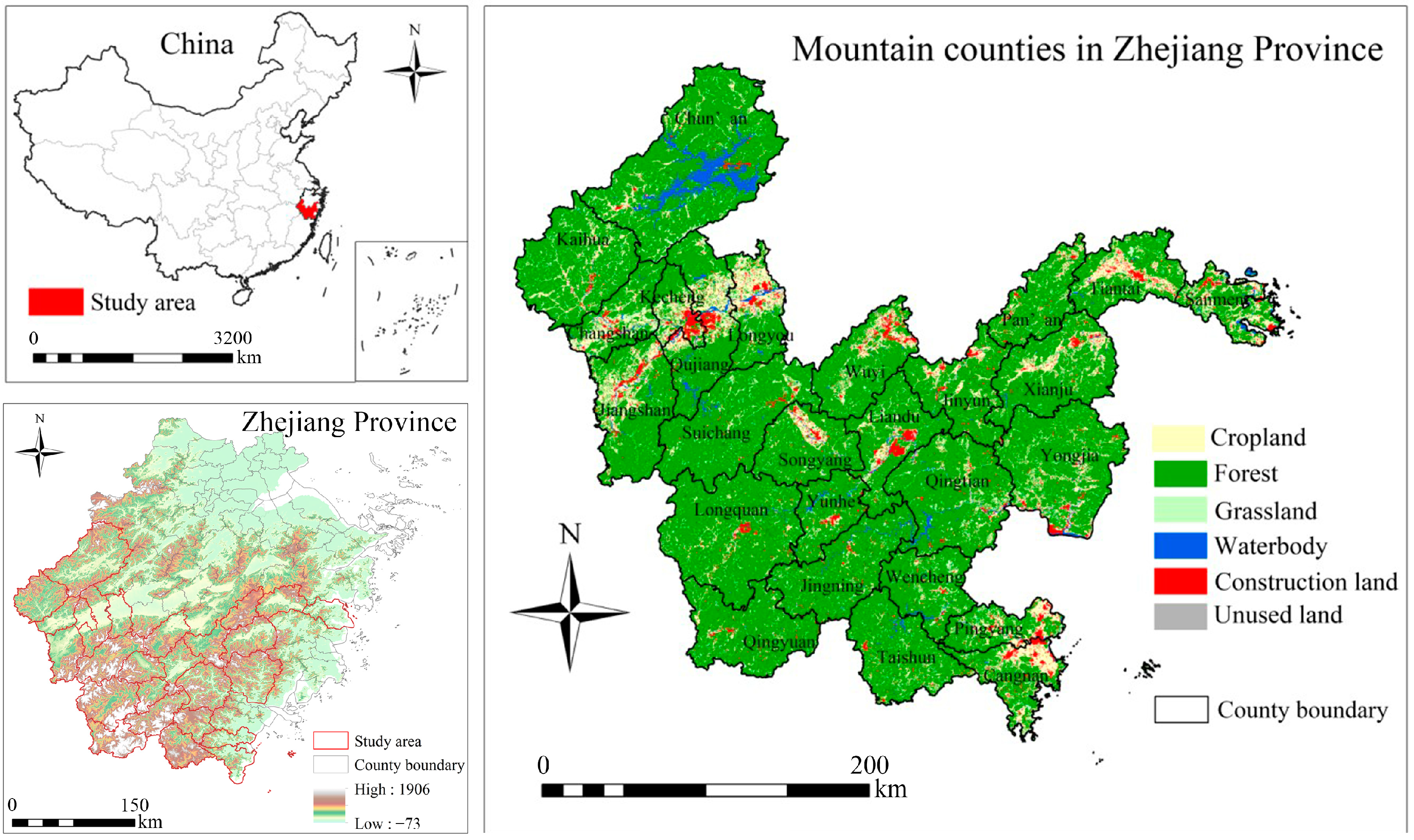
2.1. Study Area

The MC region lies between 27°06′ N–30°2′ N and 118°1′ E–121°56′ E in the southern Zhejiang Province. It covers an area of 45,707 km2, accounting for 43.5% of Zhejiang Province (Figure 1). Zhejiang has promoted the development of less-developed areas as the strategic focus of the province’s modernization. In 2001, the government, for the first time, specified that the less-developed areas included all 16 counties in Quzhou and Lishui City, as well as Taishun, Wencheng, Yongjia, Cangnan, Pan’an, Wuyi, Sanmen, Xianju, Tiantai, and Chun’an counties. In 2005, the objective increased to Pingyang County, namely the 26 mountainous counties.
The study area has a typical subtropical monsoon climate, with an annual average temperature range of 15 to 18 °C and an annual average precipitation of 1100 to 2000 mm. The elevation decreases from southwest to northeast, ranging from 1911 m to 0 m above sea level. Zhejiang’s forest coverage is about 61%. In contrast, the forest coverage in the study area exceeds 76%. The total GDP of the MC region was CNY 591.6 billion in 2020, accounting for 10.6% of the total GDP of the province. The permanent resident population at the end of 2020 was 10.17 million people, accounting for 17% of the province’s total population. The per capita GDP is about CNY 62,100, less than 68.8% of the province’s per capita GDP.

2.2. Data Sources

Data mainly included: (1) The classification of terrestrial ecosystems in Zhejiang Province was based on the 30 m × 30 m land-cover dataset of the Chinese Academy of Sciences (https://www.resdc.cn/) accessed on 20 April 2022. (2) Digital elevation model (DEM) data were derived from the Geospatial Data Cloud, Chinese Academy of Sciences (https://www.gscloud.cn/) accessed on 22 April 2022. (3) Net Primary Production (NPP) was extracted from MODIS/Terra Net Primary Production Gap-filled Yearly L4 Global 500 m SIN Grid (MOD17A3HGF), which was supplied by NASA-USGA (https://lpdaac.usgs.gov/) accessed on 17 May 2022. (4) The normalized difference vegetation index (NDVI) data were extracted from the MODIS/Terra Vegetation Indices 16-Day L3 Global 250 m SIN Grid (MOD13Q1). We calculated annual NDVI data using the maximum value composite method, which was used to generate the vegetation cover factor. (5) Hydrology-related spatial data were produced by the Department of Water Resources of Zhejiang Province. The runoff coefficient for different ecosystems was adopted from the previous study [45]. (6) Meteorological data, including precipitation and evaporation with a spatial resolution of 1 km × 1 km (rainstorm), were obtained from the Meteorological Bureau of Zhejiang Province. (7) Statistical data, such as grain output, were obtained from the Zhejiang Statistical Yearbook.

3. Methods

3.1. Quantifying Multiple ESs

In this study, we identified five ES types based on the following three criteria: (1) The selected ESs should be closely related to human well-being in the MC region. The study area belonged to a water conservation zone in the main function regionalization of China [46], and it was located in a mountainous area, with high carbon sequestration and soil retention. Lakes and reservoirs are densely distributed and have high flood mitigation. We also considered food production services that directly benefit local residents. (2) The data needed to calculate the selected ESs should be available. (3) The selected ESs should be significantly affected by human activities and socio-economic development. Based on this, five key ESs (food production, FP; water conservation, WC; soil retention; carbon sequestration, CS; flood mitigation, FM) were proposed to be selected for use in the MC region.

3.1.1. FP

Food production is a key ES for food security and sustainable development. The food supply in the study area mainly comes from cultivated land, involving grain, beans, oil, and vegetables. We recognized cultivated land as the main land-use type providing food production, and there existed a linear relationship between food production and NPP [47]. We extracted the NPP of each grid by the average value in August, which reflected the best growth status. Then, the food crop production of the whole county was allocated to the farmland grids according to the NPP as follows [48]:
F i = N P P i j × G j N P P s u m , j
where Fi is the food production in pixel i (t), NPPij is the farmland NPP in pixel i in county j (t), NPPsum,j is the total value of farmland NPP in county j (t), and Gij is the grain yield in county j (t).

3.1.2. WC

Water conservation refers to water held by forest, shrub, grassland, and wetland ecosystems from precipitation. We counted the quantity of annual water conservation by using water balance model, and runoff coefficient values were obtained from the previous study [49].
Q wc = i = 1 n A i × ( P i R i ET i ) × 10 3
where Qwc is the quantity of water (m3·a−1) conserved by an ecosystem, Ai is the area of the ecosystem i (m2), Pi is the precipitation of the ecosystem i (mm·a−1), Ri is the runoff of the ecosystem i (mm·a−1), which is related to precipitation using the runoff coefficient, ETi is the evapotranspiration of the ecosystem i (mm·a−1), and n is the number of ecosystem types.

3.1.3. SR

Soil retention is a function of the ecosystem that holds soil in place to keep it contained. Due to the large amount of hills and mountains, abundant rainfall, and anthropogenic activity in the MC region, soil erosion has become one of the major problems, resulting in the loss of limited arable land. Therefore, soil retention is an important ecosystem service that should be valued in the study area. We used the Revised Universal Soil Loss Equation (RUSLE), which can be expressed as follows [50]:
Q sr = i = 1 n R   ×   K   ×   L   × S   ×   1   -   C   ×   A i
where Qsr represents the amount of soil (t·a−1) held by the ecosystem. R is the rainfall erosivity factor (MJ·mm ·ha−1·h−1·a−1) based on monthly rainfall, K is the soil erodibility factor (t·ha·h·ha−1·MJ−1·mm−1) derived from Zhang et al. [51], L is the slope length factor, S is the steepness factor calculated by ARCGIS 10.2, C is the vegetation cover factor [52], Ai is the area of the ecosystem i (m2), and n is the number of ecosystem types.

3.1.4. CS

Carbon sequestration refers to the long-term capture and storage of atmospheric carbon dioxide in terrestrial ecosystems. NPP is one of the factors that can reflect the total amount of CO2 that is sequestrated [53]. In this study, we calculated the amount of sequestrated carbon as follows:
Q CO 2 = M CO 2 / M C × α   × NPP
where Q CO 2 is the quantity of the sequestrated carbon (t·CO2·a−1) by certain ecosystem, M CO 2 / M C is the ratio of CO2 and C, α is the conversion coefficients of net ecosystem production (NEP) and NPP [54], and NPP is the annual net primary productivity (t·C·a−1).

3.1.5. FM

Flood mitigation refers to the storage capacity of ecosystems, which can store excess water flows during flooding. Ecosystems such as forests, lakes, marshes, and reservoirs can store water and affect the timing and magnitude of water flows and runoff, intercepting heavy rainfall and absorbing water through roots and storage capacity [55]. Regardless of no marsh land cover in this study area, we measured flood mitigation based on the runoff retention by natural vegetation, lakes, and reservoirs [56].
Qfm = Qfc + Qlc + Qrc
where Qfm is the annual quantity of flood mitigation provided by the ecosystem (m3·a−1), and Qfc, Qlc, and Qrc are the annual quantity of flood mitigation from natural vegetation, lakes, and reservoirs, respectively (m3·a−1). The raster calculation results of Qfc, Qlc, and Qrc were applied to the raster calculator in ARCGIS 10.2 for raster superposition to obtain Qfm.
For natural vegetation, the quantity of flood mitigation from natural vegetation was measured as the difference between runoff without and under vegetation cover. We calculated the quantity of flood mitigation as follows:
Q fc = i = 1 n P i R fi × A i × 10 3
R fi = P i × β i
where Pi is the precipitation of ecosystem i (mm·a−1), Ri is the runoff of ecosystem i (mm·a−1), βi is the average surface storm runoff coefficient of ecosystem i [57], Ai is the area of ecosystem i (km2), and n is the amount of ecosystem types.
For lakes, we calculated the quantity of flood mitigation from lakes based on the relationship between storage capacity and lake area. For lakes in Zhejiang, the relationship was constructed as follows:
Q lc = i = 0 n e 4.924 × A i 1.128 × 3.19
where Ai is the area of lake i (km2), and n is the total number of lakes.
For reservoirs, the flood control storage capacity was used as the quantity of flood mitigation from reservoirs.

3.2. Selection and Calculation of Landscape Pattern Metrics

According to previous studies, changes in landscape patterns affect various ecological processes and functions, ultimately leading to changes in ecosystem services [58]. Based on existing studies and combined with the actual situation of the study area [8,9,58,59], seven landscape pattern metrics were selected for analysis, i.e., the proportion of cropland (cropland%), proportion of forest (forest%), proportion of construction land (construction land%), patch density (PD), cohesion (COHE), landscape shape index (LSI), and Shannon’s diversity index (SHDI), respectively. Among them, cropland%, forest%, and construction land% were landscape composition indicators, which represented the dominant type of regional land use. PD, COHE, LSI, and SHDI were landscape configuration indicators. Descriptions of all indicators are provided in Table 1.

3.3. Analyzing Trade-Offs and Synergies of ESs at Different Scales

To identify the quantitative correlations between different ESs, Pearson correlation analysis was used to reveal the interactive relationships between ESs. A correlation analysis was conducted at the grid, watershed, town, and county scales, and the mean value of each ES in each unit was determined.
To further reveal the spatial interactive relationships between ESs, the spatial overlay analysis was introduced to reveal the TOSs among the multiple services. First, the value of each ES category was divided into three levels using the natural break classification method, namely low (L = 1), medium (M = 2), and high (H = 3). Then, the raster data of the five ecosystem services were overlaid as follows:
CODE = FM × 10,000 + SR×1000 + WC × 100 + CS × 10 + FP
where FM, SR, WC, CS, and FP represent flood mitigation, soil retention, water conversation, carbon sequestration, and food production, respectively. CODE is a five-digit code, representing the supply capacity of the corresponding ES type. Table 2 lists the classification criteria for the types of TOSs.

3.4. Logistic Regression Model

An ordered logistic regression model was used to examine the TOSs of ESs and landscape patterns. A logistic regression model is a classical machine learning method. It builds a linear regression based on the Sigmoid function, which is usually used to address the problem of the multi-variable quantitative analysis of binary classification (dependent variable y = 1, 0). The logistic regression model has great advantages over support vector machines and neural network models in terms of training and recognition time. In this study, various landscape metrics (landscape composition indicators and landscape configuration indicators) were used as the independent variables, and the types of TOSs among ESs were applied as the dependent variables. The specific formula was as follows:
lg P = Z = C + B 1 X 1 + B 2 X 2 + + B n X n P = e Z 1 + e Z
where P is the probability of the types of TOSs, X is the landscape metrics, and B is the logistic regression coefficient.

4. Results

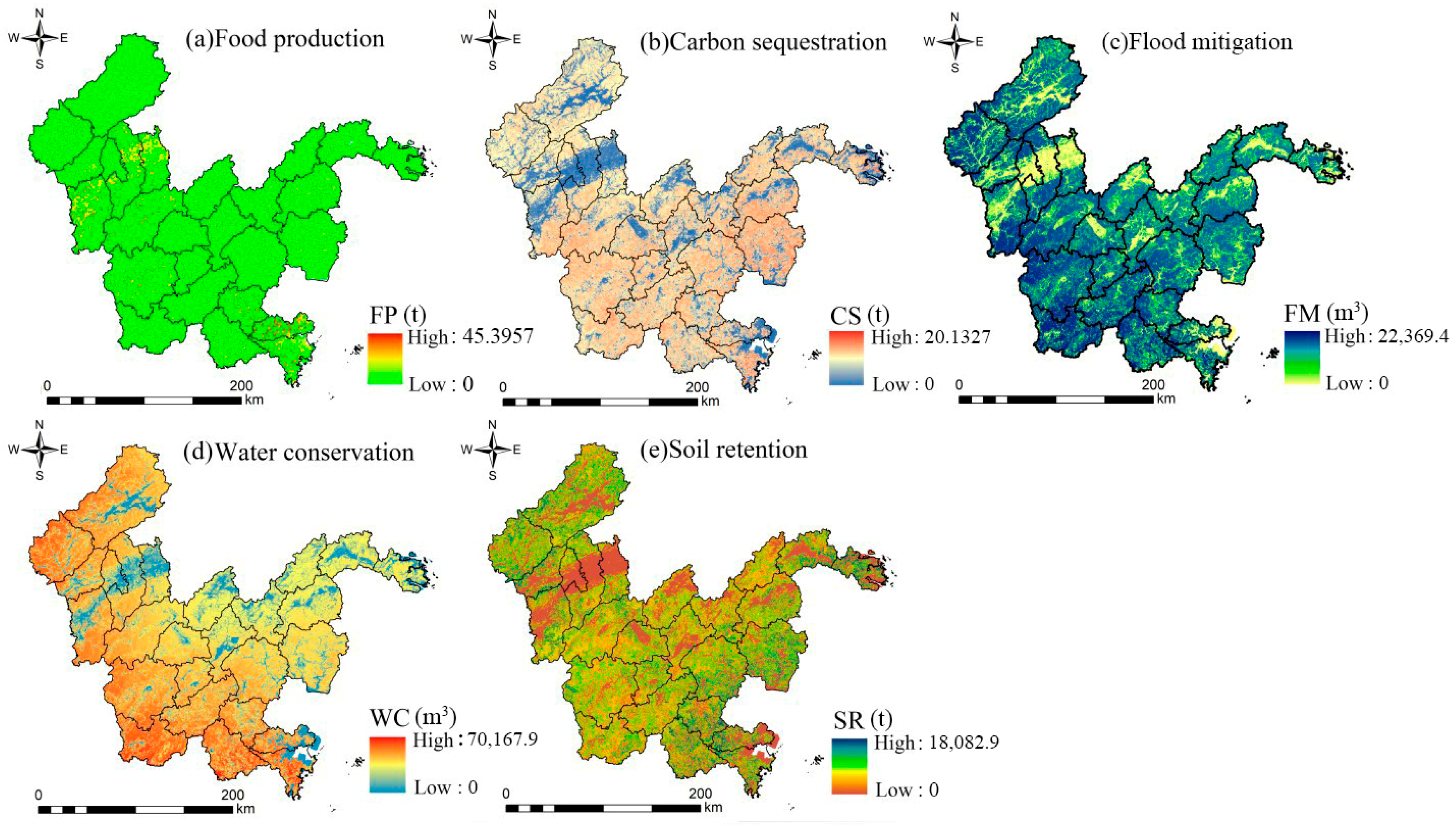
4.1. Spatial Patterns of Multiple ESs

The spatial distribution of five ESs exhibited clear heterogeneities (Figure 2). As shown in Figure 2a, food production was located in the plains in the northwest of the MC region, such as Longyou, Qujiang, and Jiangshan, as well as Pingyang and Cangnan in the eastern coastal plains. Carbon sequestration, flood mitigation, water conservation, and soil retention displayed similar spatial patterns. In detail, the values of carbon sequestration service were higher in the western parts of the study area that were covered by forest, while the values were lower in the central parts of Quzhou and the coastal areas in Cangnan and Pingyang (Figure 2b). As shown in Figure 2d, a higher water conservation value was observed in the region’s northwestern and southern regions, including Chun’an, Kaihua, Changshan, Suichang, Yunhe, Longquan, Qingyuan, Jingning, Taishun, Wencheng, and Cangnan. The high-value regions of soil retention were located in the mountainous areas that were covered with dense forest (Figure 2e).

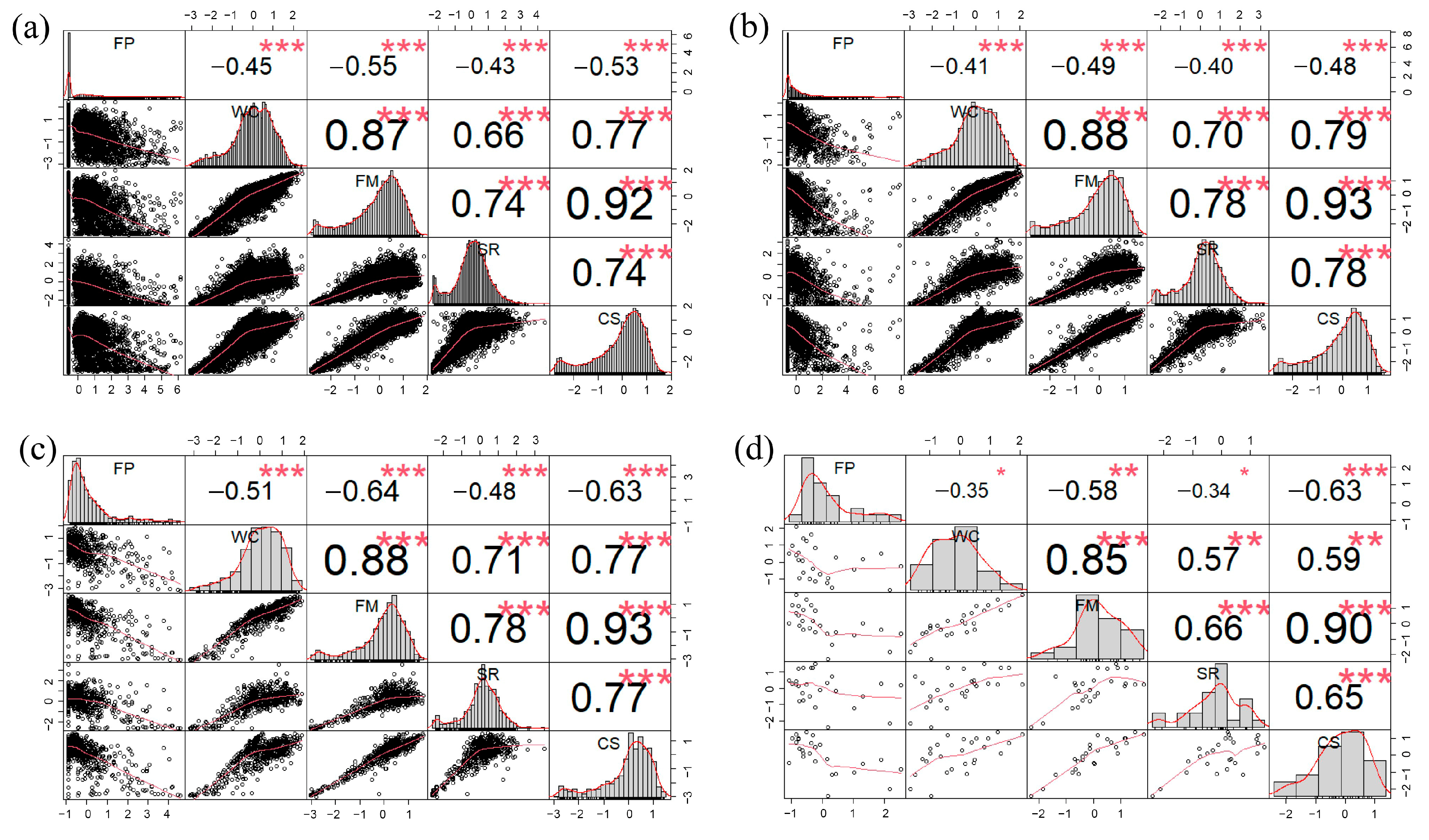
4.2. Correlation Relationships between ESs

As shown in Figure 3, significant correlations were found among 10 pairs of ESs (Pearson correlation coefficient p < 0.05; −1 < r < 1) at each scale. FP, which was negatively correlated with other ESs (p < 0.05), had a high negative correlation with FM at the grid scale (p < 0.05, r = −0.55). WC, FM, SR, and CS were positively correlated with each other, and FM was positively correlated with CS (p < 0.05, r = 0.92) and WC (p < 0.05, r = 0.87) to a great extent. When expanded to the watershed level, the correlation coefficient between FP and FM increased (p < 0.05, r = −0.49), and the positive correlations between FM and CS (p < 0.05, r = 0.93), as well as WC (p < 0.05, r = 0.88), were enhanced. At the town level, the negative correlation between FP and other ESs was stronger, while the positive correlation between WC, FM, SR, and CS showed different trends. For example, the coefficient value between FM and CS was essentially the same, the coefficient value between CS and SR decreased, and the coefficient value between WC and SR increased. The positive correlations between WC, FM, SR, and CS were all weakened when the scale was increased to the county level.

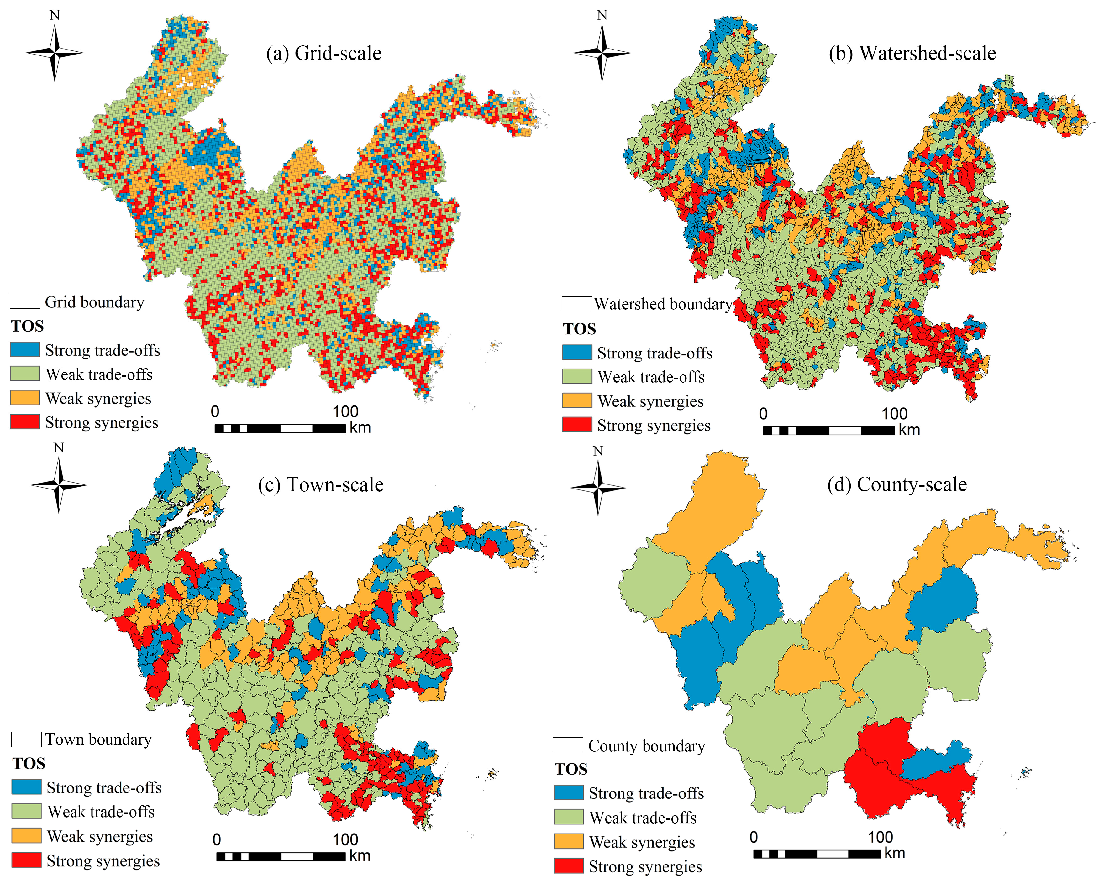
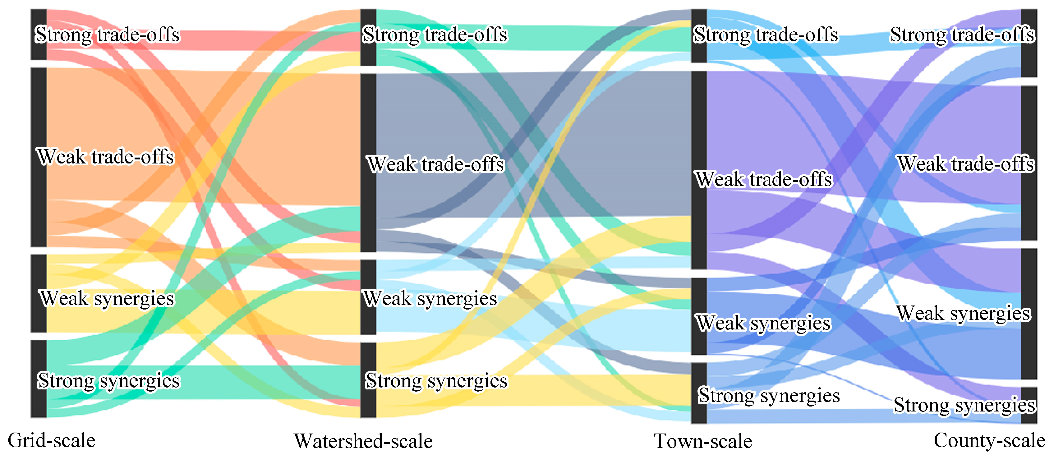
4.3. TOSs of ESs at Different Scales

Table 3 shows that weak trade-off area had the largest proportion through all scales. At the grid scale, 20.07% of ESs had strong synergies with each other and were scattered in forest ecosystems, as well as in mid-altitude hills. A total of 13.40% of ESs had strong trade-off and were distributed in agricultural and urban ecosystems (Figure 4a, Table 3). There was a total of 19.45% ESs that had strong synergies in the watershed level and were mostly located in mountainous areas of mid-low altitude in the western area and eastern coast (Figure 4b, Table 3). Table 3 and Figure 4c show that the weak trade-off area was mainly distributed in the southwest and northwest of the study region. When expanded to the county level, 34.35% of ESs had low synergies and were mainly distributed in Chun’an, Changshan, Wuyi, Songyang, Liandu, Jinyun, Pan’an, Tiantai, and Sanmen (Figure 4d, Table 3). Meanwhile, 9.24% of ESs had strong synergies and were displayed in the southern part, such as Wencheng, Taishun, and Cangnan.
In order to show the variation of trade-offs and synergies at different spatial scales, we further used a Sankey diagram to clearly represent the increase or decrease of trade-offs and synergies at the grid, watershed, town, and county scales (Figure 5). In general, the TOSs were dominated by weak trade-offs, which first increased from the grid scale to the town scale and then decreased from the town scale to the county scale (Figure 5, Table 3). The increase in weak trade-offs was mainly attributed to the inflow of strong synergies at the town scale. The weak synergies of ESs experienced a decrease from the grid scale to the watershed scale, followed by a significant increase from the town scale to the county scale. Specifically, approximately one-third of the weak synergies of ESs at the county scale came from weak trade-offs at the town scale. Strong synergies showed a decrease from the grid scale to the county scale.

4.4. The Impacts of Landscape Patterns on TOSs at Different Scales

Table 4 shows the regression coefficients of the impacts of landscape patterns at different scales, which could indicate the relationship between landscape patterns and the trade-offs/synergies of ESs. Landscape composition (i.e., cropland%, forest%, and construction land%) had a dominant impact on the trade-offs of ESs compared to spatial configuration (i.e., LSI, PD, COHE, and SHDI).
At the town scale, the results showed that cropland% had a positive effect on strong trade-offs (p < 0.01, β = 0.900), and construction land% had a positive effect on weak synergies (p < 0.01, β = 0.492). Forest% was found to have a negative impact on strong trade-offs (p < 0.01, β = −1.899). In terms of the landscape configuration, PD was negatively correlated, and COHE was positively correlated with weak trade-offs (p < 0.01, βPD =−0.831, βCOHE = 0.523).
At the watershed scale, the positive impact of cropland% and construction land% on strong trade-offs or weak synergies were both weakened (p < 0.01, βcropland% = 0.523, βconstruction land% = 0.235). Furthermore, SHDI was found to have a positive effect on strong trade-offs (p < 0.01, β = 0.954). COHE was positively correlated with strong trade-offs (β = 1.421, p < 0.01).
At the 3000 m grid scale, the negative impact of forest% on strong trade-offs was weakened (p < 0.01, β = −0.522), but its positive impact on strong synergies enhanced obviously (p < 0.01, β = 1.542). Additionally, the negative impact of construction land% on strong synergies increased (p < 0.01, β = −0.833). In terms of landscape configuration, COHE was found to have a positive effect on strong synergies (p < 0.01, β = 0.718). The impacts of PD and SHDI on strong trade-offs were both weakened (p < 0.01, βPD = 0.221, βSHDI = −0.37).

5. Discussion

Our research provided a multiscale approach to clarify the effect of landscape pattern on TOSs among ESs at different scales. Our findings enrich existing knowledge on the scale-dependent changes of ESs and TOSs, shedding new light on how landscape patterns affected TOSs at various scales, and it provides insights on integrating scale dependence into the sustainable hierarchical governance of ESs [60,61].

5.1. Multiscale Characteristics of ESs Trade-Offs and Synergies

Scale is a key factor affecting the ES characteristics and TOSs because of the unconformity of ecological conditions and processes at different scales or because of the spatial mismatch between the supply and demand of ESs [7,11,62,63]. Combined with the results of this paper, we found that there were distinct differences in the TOSs of ESs at different scales. The synergies between FM-CS and FM-WC increased when the scale expanded from grid to watershed (Figure 3). The spatial overlay results showed that the weak synergies of ESs experienced an increase from town scale to county scale (Figure 5, Table 1). These results were supported by Yang et al. (2021), who found that the ES synergies enhanced as the scale increased, and this may be attributed to the ‘peak cutting and valley filling’ process of map scale synthesis. In addition, the synergies between CS and SR decreased from watershed level to county level (Figure 3), and the strong synergies of ESs showed a continuous decrease from grid-scale to county-scale (Figure 5, Table 1). This was similar to the study of Su et al. (2020), who found that ES synergies between sediment retention and water yield decreased with the increasing scale. The reason may be due to the gradual impact of socio-economic factors such as agricultural production, population, and non-agricultural output on ESs as the scale increases [63]. The changes in the significance of the relationships among ESs illustrated that the potential TOSs between some ESs could be obscured at larger spatial scales [64,65,66,67].
While correlation analysis can calculate the trade-offs or synergies among ESs, it can hide the spatial heterogeneity of ES’s relationships [68,69]. For example, the correlation results showed that 10 pairs of ES relationships between the five ESs types were robust across scales (Figure 3) mainly due to land-use consistency [13,28,66]. However, the spatial overlay results showed that changing the scale can enhance, weaken, or even reverse the interaction between ESs (Figure 5), which suggested that the relationship of ESs changed both in direction and strength across scales [70,71]. For example, approximately one-third of the weak synergies of ESs at the county scale came from weak trade-offs at the town scale. This illustrated that the optimal management of ecosystems can transform trade-offs at the regional scale into opportunities for synergistic enhancement between ESs at the local scale [72].
The trade-off between ecosystem services is spatially heterogeneous and changes with the passage of spatial scales [73]. Therefore, there is a need to link scale effects with specific geographical environments to provide insights for cross-scale ecosystem management and sustainable spatial planning [72,74,75]. According to our methods, weak synergies meant that at least one service was low (L) and lacking ESs at the high (H) level, which underlined the necessity of land management. As areas with weak synergies were mostly located in a region with a relatively developed economy and intensive human activities, food production and regulating services were both at a relatively low level (Figure 2 and Figure 4). Therefore, for these areas, on the one hand, it is necessary to strengthen the management of land-use types, especially at the county scale, set up ecological red lines [76], implement the Grain for Green Project (GFGP) [77], improve the supply capacity of stock, carbon sequestration, water conservation, and flood mitigation services, and alleviate the strong trade-off between services. On the other hand, the government could improve the utilization rate of water and soil resources through scientific irrigation and farming methods, aiming to achieve the high yield, high quality, and high efficiency of crops.

5.2. Multiscale Analysis of the Effects of Landscape Pattern on the Trade-Offs and Synergies

Analyzing the relationship between the TOSs among ESs and the landscape pattern can be a new approach to improving and coordinating ESs [9]. This study analyzed the effect of landscape patterns on TOSs by setting multiple scales. The results showed that the direction of the influence of landscape pattern on TOSs did not change, but the magnitudes of the impacts were scale-dependent.
The findings of this study showed that landscape composition and spatial configuration had significant impacts on the TOSs of ESs, especially landscape composition (Table 3). This might be because landscape composition affected ESs by directly changing the underlying surface, which increases the competition of ESs [17]. In particular, cropland was positively correlated with the strong trade-offs of ESs (Table 3) because the use of cropland under the pressure of human demand pays more attention to food production, a large amount of fertilizers, pesticides, and high-intensity cropland utilization models, leading to the destruction of cropland ecosystems and resulting in the decline of the WC, SR, and CS of cropland. However, in the ecologically dominant functional area, cropland was negatively correlated with the weak trade-offs of ESs, indicating that cropland may be conducive to alleviate the potential conflict between ESs in ecologically sensitive areas (Figure 4, Table 3). It could be explained by the fact that the cropland in these areas is mainly used by plantations, and the planting of a large number of trees increases vegetation coverage to a certain extent, which can improve the regulation and regulation services [78]. Furthermore, the effect of forest area on the trade-offs of ESs is opposite to that of cropland (Table 3), indicating that the impact of forest and cropland on ESs changed in mountainous areas and was at a trade-off condition, which needs addressed to alleviate the conflict between farming and forestry. Fragmented landscapes can hinder inter-regional energy flows and alter nutrient cycling processes, thereby alleviating ecosystem services [79]. PD and SHDI had a positive impact on the strong trade-offs at the watershed scale. This might be because the expansion of construction land and cropland in the areas with strong ES trade-offs led to the increase of PD and SHDI, which could destroy the natural habitats and reduce the ecosystem functions [80,81].
The magnitudes of impact of landscape composition (i.e., cropland%, forest%, and construction land%) were strengthened at larger scales. Specifically, the influence of cropland% (positive) and forest% (negative) on strong trade-offs increased simultaneously from the grid scale to the town scale, and construction land% had a stronger negative impact on high synergies from the watershed scale to the town scale. The main reason was that landscape composition changed when grid cells were aggregated to large scales due to the ‘peak cutting and valley filling’ process, thus determining the ecological effects at each scale [82,83]. According to Figure 4, 13.40% of ESs had strong trade-offs and were distributed in agricultural and urban ecosystems. Specifically, most of the area was located in the middle and lower reaches of the river, which was suitable for providing food production services. However, due to the relatively gentle topography and frequent human activities, the forest stands have poor quality, mainly consisting of secondary forests and artificial plantations of young ages [42]. Therefore, the supply capacities of the CS, SR, FM, and WC were relatively low, resulting in prominent strong trade-offs. In order to alleviate the strong trade-off among these services, policy makers should strengthen the management of secondary forests and plantation forests at the town scale, promote mixed coniferous and broadleaved forests to replace pure forests, and improve the supply capacity of CS, SR, and WC [29]. Nevertheless, at the 3000-m grid scale, construction land% had the strongest impact on high synergies of ESs. This may be because the areas with high synergies were mainly distributed in forest-dominated areas (Figure 1 and Figure 4), and the construction land expansion in these areas directly led to the reduction and fragmentation of natural habitats, resulting in the degeneration of SR and CS [8,84].
The effect of various landscape configuration factors on the different TOSs of ESs was complex as the scale changed. As the scale rose to the town scale, the negative impact of COHE on weak synergies was strengthened. COHE is an indicator of physical connectivity between patch types, and a higher value indicates better connectivity between patches [21]. Therefore, the advantage of COHE can be maximized for landscape configuration planning at the town scale. When the scale increased from the grid scale to the watershed scale, the impact of LSI on the strong trade-offs of ESs was strengthened. The main reason was that landscape pattern indices changed with different scales, and in the process of small-scale transformation to large-scale, the size and current situation of the study unit changed significantly, and the shape of the landscape became complex, thus causing the change of LSI [27,85]. These findings suggest a more precise and detailed landscape configuration design to better assist the synergetic ecosystem services. According to the spatial heterogeneity of ESs, the sustainable planning strategies of landscapes should be adopted in different scales. Emphasis should be placed on improving grain production services, avoiding disorderly expansion and the fragmented development of construction land, and increasing spatial aggregation [16].

5.3. Limitations and Future Work

This research provided a deep understand of the relationships between landscape patterns and TOSs of ESs under various spatial scales in the southern Zhejiang Province of China. These findings may lead to additional knowledge that will provide more operational options for the hierarchical governance of ESs. For landscape compositions, administrative regions (i.e., town level) should be used as ecosystem service management units. For landscape compositions, landscape sustainable planning strategies should be adopted in administrative regions, as well as in watershed and grid scales. However, there are several limitations that need to be investigated with caution. Identifying the mechanisms driving service trade-offs between landscape patterns, natural processes (e.g., precipitation), and socioeconomic development (e.g., population) can help develop scientifically efficient management solutions. Apart from landscape patterns, other driving mechanisms of TOSs among ESs have not been quantitatively explored in this paper. Therefore, in the future, the extent and differences of the influence of landscape pattern, natural environmental factors, and socioeconomic factors on the TOSs should be explored simultaneously to clarify the main driving factors [86]. Second, multiscale spatial analysis is meaningful to identify the effective spatial scales for ES management [66]. Based on the characteristics of ecosystem landscape pattern at different scales and ecosystem trade-offs/synergies, this paper proposed hierarchical ecosystem governance at four scales according to local conditions. However, in terms of sustainable ecosystem supply and regional sustainable development, a more precise and detailed policy design needs to be made by detailed scale analysis. For example, continuous buffer scale (e.g., 5 km, 10 km, 15 km, etc.) analysis may bring a new insight in the research. Third, our study was based on data collected in 2020. The interpretation of the relationship between ESs, TOSs, landscape patterns, and temporal dynamics may be the focus of future research.

6. Conclusions

In order to develop a deeper understanding of the scale-dependent effect of landscape patterns on trade-offs and synergies among ESs, this study investigated spatial patterns, relationships between ES pairs, TOSs among the multiple ESs, and the effect of landscape pattern on the TOSs of ESs at different spatial scales in the MC region. These findings were fundamentally important for guiding local governments to refine and optimize regional TOSs, especially in developing areas that are facing a series of land-use changes because of dramatic development. The results showed that:
(1) There were distinct differences in the TOSs of ESs at different scales. The Pearson correlation results showed that 10 pairs of ES relationships were robust across scales, while the spatial overlay results showed that TOSs changed both in direction and strength across scales. The weak synergies of ESs experienced a significant increase from the town scale to the county scale, while the strong synergies of ESs showed a continuous decrease from the grid scale to the county scale.
(2) The direction of the influence of landscape pattern on TOSs did not change, but the magnitudes of the impacts were scale-dependent. Landscape composition (i.e., cropland%, forest%, and construction land%) had more significant effects on the trade-offs of ESs than spatial configuration (i.e., LSI, PD, COHE, and SHDI). The magnitudes of impact of landscape composition (i.e., cropland%, forest%, and construction land%) were strengthened at larger scales. The effects of various landscape configuration factors on the TOSs of ESs were complex as the scale changed.
(3) A more accurate and detailed landscape pattern design is proposed for sustainable landscape planning strategies across different scales. Specifically, for landscape pattern compositions, administrative regions (i.e., town level) should be used as ecosystem service management units due to the impact of landscape pattern composition on trade-off synergies at larger scales. For landscape pattern configurations, landscape sustainable planning strategies should be adopted in different scales. Emphasis should be placed on improving grain production services, avoiding disorderly expansion and the fragmented development of construction land, and increasing spatial aggregation.

Author Contributions

L.D.: data collection, software, formal analysis, visualization, writing—original draft. Y.L.: data curation. C.Z.: conceptualization, methodology, supervision. Q.Z.: conceptualization, validation. K.W.: validation, writing—review and editing. All authors have read and agreed to the published version of the manuscript.

Funding

This work was supported by the National Key Research and Development Program of China (2022YFF1301802-4), the National Natural Science Foundation of China (41971236), and Basic scientific research business cost project of Zhejiang Gongshang University (No. XT202209).

Institutional Review Board Statement

This study did not require ethical approval.

Informed Consent Statement

Not applicable.

Data Availability Statement

The authors do not have permission to share data.

Conflicts of Interest

The authors declare that they have no known competing financial interests or personal relationships that could have appeared to influence the work reported in this paper.

References

  1. Estoque, R.C.; Murayama, Y. Quantifying landscape pattern and ecosystem service value changes in four rapidly urbanizing hill stations of Southeast Asia. Landsc. Ecol. 2016, 31, 1481–1507. [Google Scholar] [CrossRef]
  2. MEA. Ecosystems and Human Well-Being: Scenarios: Findings of the Scenarios Working Group; Island Press: Washington, DC, USA, 2005. [Google Scholar]
  3. Byrd, K.B.; Flint, L.E.; Alvarez, P.; Casey, C.F.; Sleeter, B.M.; Soulard, C.E.; Flint, A.L.; Sohl, T.L. Integrated climate and land use change scenarios for California rangeland ecosystem services: Wildlife habitat, soil carbon, and water supply. Landsc. Ecol. 2015, 30, 729–750. [Google Scholar] [CrossRef]
  4. Cai, W.; Peng, W. Exploring Spatiotemporal Variation of Carbon Storage Driven by Land Use Policy in the Yangtze River Delta Region. Land 2021, 10, 1120. [Google Scholar] [CrossRef]
  5. Addisie, M.B.B.; Molla, G.; Teshome, M.; Ayele, G.T.T. Evaluating Biophysical Conservation Practices with Dynamic Land Use and Land Cover in the Highlands of Ethiopia. Land 2022, 11, 2187. [Google Scholar] [CrossRef]
  6. Mohammadyari, F.; Zarandian, A.; Mirsanjari, M.M.; Suziedelyte Visockiene, J.; Tumeliene, E. Modelling Impact of Urban Expansion on Ecosystem Services: A Scenario-Based Approach in a Mixed Natural/Urbanised Landscape. Land 2023, 12, 291. [Google Scholar] [CrossRef]
  7. Cord, A.F.; Bartkowski, B.; Beckmann, M.; Dittrich, A.; Hermans-Neumann, K.; Kaim, A.; Lienhoop, N.; Locher-Krause, K.; Priess, J.; Schroter-Schlaack, C.; et al. Towards systematic analyses of ecosystem service trade-offs and synergies: Main concepts, methods and the road ahead. Ecosyst. Serv. 2017, 28, 264–272. [Google Scholar] [CrossRef]
  8. Zhu, C.; Zhang, X.; Zhou, M.; He, S.; Gan, M.; Yang, L.; Wang, K. Impacts of urbanization and landscape pattern on habitat quality using OLS and GWR models in Hangzhou, China. Ecol. Indic. 2020, 117, 106654. [Google Scholar] [CrossRef]
  9. Liu, S.; Wang, Z.; Wu, W.; Yu, L. Effects of landscape pattern change on ecosystem services and its interactions in karst cities: A case study of Guiyang City in China. Ecol. Indic. 2022, 145, 109646. [Google Scholar] [CrossRef]
  10. Lyu, R.; Zhao, W.; Tian, X.; Zhang, J. Non-linearity impacts of landscape pattern on ecosystem services and their trade-offs: A case study in the City Belt along the Yellow River in Ningxia, China. Ecol. Indic. 2022, 136, 108608. [Google Scholar] [CrossRef]
  11. Peng, J.; Hu, X.; Zhao, M.; Liu, Y.; Tian, L. Research progress on ecosystem service trade-offs: From cognition to decision-making. Acta Geogr. Sin. 2017, 72, 960–973. [Google Scholar]
  12. Wu, J.G. Effects of changing scale on landscape pattern analysis: Scaling relations. Landsc. Ecol. 2004, 19, 125–138. [Google Scholar] [CrossRef]
  13. Li, K.; Chen, J.; Lin, J.; Zhang, H.; Xie, Y.; Li, Z.; Wang, L. Identifying Ecosystem Service Trade-Offs and Their Response to Landscape Patterns at Different Scales in an Agricultural Basin in Central China. Land 2022, 11, 1336. [Google Scholar] [CrossRef]
  14. Yohannes, H.; Soromessa, T.; Argaw, M.; Dewan, A. Impact of landscape pattern changes on hydrological ecosystem services in the Beressa watershed of the Blue Nile Basin in Ethiopia. Sci. Total Environ. 2021, 793, 148559. [Google Scholar] [CrossRef]
  15. Hao, R.F.; Yu, D.Y.; Liu, Y.P.; Liu, Y.; Qiao, J.M.; Wang, X.; Du, J.S. Impacts of changes in climate and landscape pattern on ecosystem services. Sci. Total Environ. 2017, 579, 718–728. [Google Scholar] [CrossRef] [PubMed]
  16. Li, J.; Zhou, K.; Xie, B.; Xiao, J. Impact of landscape pattern change on water-related ecosystem services: Comprehensive analysis based on heterogeneity perspective. Ecol. Indic. 2021, 133, 108372. [Google Scholar] [CrossRef]
  17. Lamy, T.; Liss, K.N.; Gonzalez, A.; Bennett, E.M. Landscape structure affects the provision of multiple ecosystem services. Environ. Res. Lett. 2016, 11, 124017. [Google Scholar] [CrossRef]
  18. Yang, W.; Jin, Y.; Sun, T.; Yang, Z.; Cai, Y.; Yi, Y. Trade-offs among ecosystem services in coastal wetlands under the effects of reclamation activities. Ecol. Indic. 2018, 92, 354–366. [Google Scholar] [CrossRef]
  19. Tran, D.X.; Pearson, D.; Palmer, A.; Lowry, J.; Gray, D.; Dominati, E.J. Quantifying spatial non-stationarity in the relationship between landscape structure and the provision of ecosystem services: An example in the New Zealand hill country. Sci. Total Environ. 2022, 808, 152126. [Google Scholar] [CrossRef]
  20. Zhang, J.; Qu, M.; Wang, C.; Zhao, J.; Cao, Y. Quantifying landscape pattern and ecosystem service value changes: A case study at the county level in the Chinese Loess Plateau. Glob. Ecol. Conserv. 2020, 23, e01110. [Google Scholar] [CrossRef]
  21. Wu, J.G. Landscape sustainability science: Ecosystem services and human well-being in changing landscapes. Landsc. Ecol. 2013, 28, 999–1023. [Google Scholar] [CrossRef]
  22. Chen, W.; Chi, G.; Li, J. The spatial association of ecosystem services with land use and land cover change at the county level in China, 1995–2015. Sci. Total Environ. 2019, 669, 459–470. [Google Scholar] [CrossRef]
  23. Luo, Y.; Lu, Y.; Fu, B.; Zhang, Q.; Li, T.; Hu, W.; Comber, A. Half century change of interactions among ecosystem services driven by ecological restoration: Quantification and policy implications at a watershed scale in the Chinese Loess Plateau. Sci. Total Environ. 2019, 651, 2546–2557. [Google Scholar] [CrossRef] [PubMed]
  24. Li, S.; Zhao, Y.; Xiao, W.; Yellishetty, M.; Yang, D. Identifying ecosystem service bundles and the spatiotemporal characteristics of trade-offs and synergies in coal mining areas with a high groundwater table. Sci. Total Environ. 2022, 807, 151036. [Google Scholar] [CrossRef] [PubMed]
  25. Feng, Q.; Zhao, W.; Fu, B.; Ding, J.; Wang, S. Ecosystem service trade-offs and their influencing factors: A case study in the Loess Plateau of China. Sci. Total Environ. 2017, 607, 1250–1263. [Google Scholar] [CrossRef]
  26. Hou, Y.; Lu, Y.H.; Chen, W.P.; Fu, B.J. Temporal variation and spatial scale dependency of ecosystem service interactions: A case study on the central Loess Plateau of China. Landsc. Ecol. 2017, 32, 1201–1217. [Google Scholar] [CrossRef]
  27. Li, K.M.; Li, C.L.; Liu, M.; Hu, Y.M.; Wang, H.; Wu, W. Multiscale analysis of the effects of urban green infrastructure landscape patterns on PM2.5 concentrations in an area of rapid urbanization. J. Clean. Prod. 2021, 325, 129324. [Google Scholar] [CrossRef]
  28. Yang, M.; Gao, X.; Zhao, X.; Wu, P. Scale effect and spatially explicit drivers of interactions between ecosystem services-A case study from the Loess Plateau. Sci. Total Environ. 2021, 785, 147389. [Google Scholar] [CrossRef]
  29. Zhang, J.; Zhu, W.; Zhu, L.; Li, Y. Multi-scale analysis of trade-off/synergistic effects of forest ecosystem services in the Funiu Mountain Region, China. J. Geogr. Sci. 2022, 32, 981–999. [Google Scholar] [CrossRef]
  30. Chisholm, R.A. Trade-offs between ecosystem services: Water and carbon in a biodiversity hotspot. Ecol. Econ. 2010, 69, 1973–1987. [Google Scholar] [CrossRef]
  31. Hein, L.; van Koppen, K.; de Groot, R.S.; van Ierland, E.C. Spatial scales, stakeholders and the valuation of ecosystem services. Ecol. Econ. 2006, 57, 209–228. [Google Scholar] [CrossRef]
  32. Dou, H.; Li, X.; Li, S.; Dang, D.; Li, X.; Lyu, X.; Li, M.; Liu, S. Mapping ecosystem services bundles for analyzing spatial trade-offs in inner Mongolia, China. J. Clean. Prod. 2020, 256, 120444. [Google Scholar] [CrossRef]
  33. Karimi, J.D.; Corstanje, R.; Harris, J.A. Bundling ecosystem services at a high resolution in the UK: Trade-offs and synergies in urban landscapes. Landsc. Ecol. 2021, 36, 1817–1835. [Google Scholar] [CrossRef]
  34. Lin, S.W.; Wu, R.D.; Yang, F.L.; Wang, J.J.; Wu, W. Spatial trade-offs and synergies among ecosystem services within a global biodiversity hotspot. Ecol. Indic. 2018, 84, 371–381. [Google Scholar] [CrossRef]
  35. Raudsepp-Hearne, C.; Peterson, G.D.; Bennett, E.M. Ecosystem service bundles for analyzing tradeoffs in diverse landscapes. Proc. Natl. Acad. Sci. USA 2010, 107, 5242–5247. [Google Scholar] [CrossRef] [PubMed]
  36. Turner, K.G.; Odgaard, M.V.; Bocher, P.K.; Dalgaard, T.; Svenning, J.C. Bundling ecosystem services in Denmark: Trade-offs and synergies in a cultural landscape. Landsc. Urban Plan. 2014, 125, 89–104. [Google Scholar] [CrossRef]
  37. Wu, L.; Sun, C.; Fan, F. Multi-criteria framework for identifying the trade-offs and synergies relationship of ecosystem services based on ecosystem services bundles. Ecol. Indic. 2022, 144, 109453. [Google Scholar] [CrossRef]
  38. Hao, C.; Wu, S.; Zhang, W.; Chen, Y.; Ren, Y.; Chen, X.; Wang, H.; Zhang, L. A critical review of Gross ecosystem product accounting in China: Status quo, problems and future directions. J. Environ. Manag. 2022, 322, 115995. [Google Scholar] [CrossRef]
  39. Cademus, R.; Escobedo, F.J.; McLaughlin, D.; Abd-Elrahman, A. Analyzing Trade-Offs, Synergies, and Drivers among Timber Production, Carbon Sequestration, and Water Yield in Pinus elliotii Forests in Southeastern USA. Forests 2014, 5, 1409–1431. [Google Scholar] [CrossRef]
  40. Wang, J.; Cao, Y.; Fang, X.; Li, G.; Cao, Y. Identification of the trade-offs/synergies between rural landscape services in a spatially explicit way for sustainable rural development. J. Environ. Manag. 2021, 300, 113706. [Google Scholar] [CrossRef]
  41. Zhao, X.; Ding, X.; Li, L. Research on Environmental Regulation, Technological Innovation and Green Transformation of Manufacturing Industry in the Yangtze River Economic Belt. Sustainability 2021, 13, 10005. [Google Scholar] [CrossRef]
  42. Xiong, B.; Chen, R.; An, L.; Zhang, Q.; Xia, Z. Telecoupling urbanization and mountain areas deforestation between 2000 and 2020: Evidence from Zhejiang Province, China. Land Degrad. Dev. 2021, 32, 4727–4739. [Google Scholar] [CrossRef]
  43. Rolo, V.; Roces-Diaz, J.V.; Torralba, M.; Kay, S.; Fagerholm, N.; Aviron, S.; Burgess, P.; Crous-Duran, J.; Ferreiro-Dominguez, N.; Graves, A.; et al. Mixtures of forest and agroforestry alleviate trade-offs between ecosystem services in European rural landscapes. Ecosyst. Serv. 2021, 50, 101318. [Google Scholar] [CrossRef]
  44. Sun, X.; Shan, R.; Liu, F. Spatio-temporal quantification of patterns, trade-offs and synergies among multiple hydrological ecosystem services in different topographic basins. J. Clean. Prod. 2020, 268, 122338. [Google Scholar] [CrossRef]
  45. Jin, X.; Wei, L.; Wang, Y.; Lu, Y. Construction of ecological security pattern based on the importance of ecosystem service functions and ecological sensitivity assessment: A case study in Fengxian County of Jiangsu Province, China. Environ. Dev. Sustain. 2021, 23, 563–590. [Google Scholar] [CrossRef]
  46. Ministry of Environmental Protection; Chinese Academy of Sciences. National Ecological Function Zoning. 2015. Available online: https://www.mee.gov.cn/gkml/hbb/bgg/201511/t20151126_317777.htm (accessed on 23 May 2022).
  47. Huang, Y.; Zhang, W.; Sun, W.; Zheng, X. Net primary production of Chinese croplands from 1950 to 1999. Ecol. Appl. 2007, 17, 692–701. [Google Scholar] [CrossRef]
  48. Liu, C.; Xu, Y.; Huang, A.; Li, Y.; Wang, H.; Lu, L.; Sun, P.; Zheng, W. Spatial identification of land use multifunctionality at grid scale in farming-pastoral area: A case study of Zhangjiakou City, China. Habitat Int. 2018, 76, 48–61. [Google Scholar] [CrossRef]
  49. Ouyang, Z.; Zheng, H.; Xiao, Y.; Polasky, S.; Liu, J.; Xu, W.; Wang, Q.; Zhang, L.; Xiao, Y.; Rao, E.M.; et al. Improvements in ecosystem services from investments in natural capital. Science 2016, 352, 1455–1459. [Google Scholar] [CrossRef]
  50. Rao, E.; Ouyang, Z.; Yu, X.; Xiao, Y. Spatial patterns and impacts of soil conservation service in China. Geomorphology 2014, 207, 64–70. [Google Scholar] [CrossRef]
  51. Zhang, K.; Peng, W.; Yang, H. Soilerodibility and its estimation for agricultural soils in China. Acta Pedol. Sin. 2007, 44, 7–13. [Google Scholar]
  52. Wei, H.; Li, R.; Yang, Q. Research advances of vegetation effect on soil and water conservation in China. Acta Phytoecol. Sin. 2002, 26, 489–496. [Google Scholar]
  53. Wu, Y.; Wang, P.; Liu, X.; Chen, J.; Song, M. Analysis of regional carbon allocation and carbon trading based on net primary productivity in China. China Econ. Rev. 2020, 60, 101401. [Google Scholar] [CrossRef]
  54. Chinese Academy of Environmental Planning, Research Center for Eco-Environmental Sciences. The Technical Guideline on Cross Ecosystem Product (GEP). 2020. Available online: http://www.caep.org.cn/zclm/sthjyjjhszx/zxdt_21932/202010/t20201029_805419.shtml (accessed on 26 April 2022).
  55. Xiao, Y.; Ouyang, Z.; Xu, W.; Xiao, Y.; Zheng, H.; Xian, C. Optimizing hotspot areas for ecological planning and management based on biodiversity and ecosystem services. Chin. Geogr. Sci. 2016, 26, 256–269. [Google Scholar] [CrossRef]
  56. Zhejiang Provincial Market Supervision Administration. Technical Specification for Accounting Gross Ecosystem Product (GEP)—Terrestrial Ecosystems. 2020, DB33/T 2274—2020. Available online: http://zjamr.zj.gov.cn/art/2020/9/29/art_1229047334_58814039.html (accessed on 25 April 2022).
  57. Fu, B.; Wang, Y.K.; Xu, P.; Yan, K. Mapping the Flood Mitigation Services of Ecosystems—A Case Study in the Upper Yangtze River Basin. Ecol. Eng. 2013, 52, 238–246. [Google Scholar] [CrossRef]
  58. Duan, X.; Chen, Y.; Wang, L.; Zheng, G.; Liang, T. The impact of land use and land cover changes on the landscape pattern and ecosystem service value in Sanjiangyuan region of the Qinghai-Tibet Plateau. J. Environ. Manag. 2022, 325, 116539. [Google Scholar] [CrossRef] [PubMed]
  59. Zhou, J.; Luo, C.; Ma, D.; Shi, W.; Wang, L.; Guo, Z.; Tang, H.; Wang, X.; Wang, J.; Liu, C.; et al. The impact of land use landscape pattern on river hydrochemistry at multi-scale in an inland river basin, China. Ecol. Indic. 2022, 143, 109334. [Google Scholar] [CrossRef]
  60. Deng, X.; Li, Z.; Gibson, J. A review on trade-off analysis of ecosystem services for sustainable land-use management. J. Geogr. Sci. 2016, 26, 953–968. [Google Scholar] [CrossRef]
  61. Haines-Young, R.; Potschin, M.; Kienast, F. Indicators of ecosystem service potential at European scales: Mapping marginal changes and trade-offs. Ecol. Indic. 2012, 21, 39–53. [Google Scholar] [CrossRef]
  62. Shen, J.; Li, S.; Liu, L.; Liang, Z.; Wang, Y.; Wang, H.; Wu, S. Uncovering the relationships between ecosystem services and social- ecological drivers at different spatial scales in the Beijing-Tianjin- Hebei region. J. Clean. Prod. 2021, 290, 125193. [Google Scholar] [CrossRef]
  63. Su, C.; Dong, M.; Fu, B.; Liu, G. Scale effects of sediment retention, water yield, and net primary production: A case-study of the Chinese Loess Plateau. Land Degrad. Dev. 2020, 31, 1408–1421. [Google Scholar] [CrossRef]
  64. Bai, Y.; Chen, Y.; Alatalod, J.M.; Yang, Z.; Jiang, B. Scale effects on the relationships between land characteristics and ecosystem services- a case study in Taihu Lake Basin, China. Sci. Total Environ. 2020, 716, 137083. [Google Scholar] [CrossRef]
  65. Spake, R.; Lasseur, R.; Crouzat, E.; Bullock, J.M.; Lavorel, S.; Parks, K.E.; Schaafsma, M.; Bennett, E.M.; Maes, J.; Mulligan, M.; et al. Unpacking ecosystem service bundles: Towards predictive mapping of synergies and trade-offs between ecosystem services. Glob. Environ. Chang.-Hum. Policy Dimens. 2017, 47, 37–50. [Google Scholar] [CrossRef]
  66. Xu, S.; Liu, Y.; Wang, X.; Zhang, G. Scale effect on spatial patterns of ecosystem services and associations among them in semi-arid area: A case study in Ningxia Hui Autonomous Region, China. Sci. Total Environ. 2017, 598, 297–306. [Google Scholar] [CrossRef] [PubMed]
  67. Yang, G.F.; Ge, Y.; Xue, H.; Yang, W.; Shi, Y.; Peng, C.H.; Du, Y.Y.; Fan, X.; Ren, Y.; Chang, J. Using ecosystem service bundles to detect trade-offs and synergies across urban-rural complexes. Landsc. Urban Plan. 2015, 136, 110–121. [Google Scholar] [CrossRef]
  68. Maes, J.; Paracchini, M.L.; Zulian, G.; Dunbar, M.B.; Alkemade, R. Synergies and trade-offs between ecosystem service supply, biodiversity, and habitat conservation status in Europe. Biol. Conserv. 2012, 155, 1–12. [Google Scholar] [CrossRef]
  69. Tomscha, S.A.; Gergel, S.E. Ecosystem service trade-offs and synergies misunderstood without landscape history. Ecol. Soc. 2016, 21, 43. [Google Scholar] [CrossRef]
  70. Wang, H.; Liu, L.; Yin, L.; Shen, J.; Li, S. Exploring the complex relationships and drivers of ecosystem services across different geomorphological types in the Beijing-Tianjin-Hebei region, China (2000–2018). Ecol. Indic. 2021, 121, 107116. [Google Scholar] [CrossRef]
  71. Wang, Y.; Li, X.; Zhang, Q.; Li, J.; Zhou, X. Projections of future land use changes: Multiple scenarios -based impacts analysis on ecosystem services for Wuhan city, China. Ecol. Indic. 2018, 94, 430–445. [Google Scholar] [CrossRef]
  72. Bennett, E.M.; Cramer, W.; Begossi, A.; Cundill, G.; Diaz, S.; Egoh, B.N.; Geijzendorffer, I.R.; Krug, C.B.; Lavorel, S.; Lazos, E.; et al. Linking biodiversity, ecosystem services, and human well-being: Three challenges for designing research for sustainability. Curr. Opin. Environ. Sustain. 2015, 14, 76–85. [Google Scholar] [CrossRef]
  73. Su, C.; Fu, B. Evolution of ecosystem services in the Chinese Loess Plateau under climatic and land use changes. Glob. Planet. Chang. 2013, 101, 119–128. [Google Scholar] [CrossRef]
  74. Raudsepp-Hearne, C.; Peterson, G.D. Scale and ecosystem services: How do observation, management, and analysis shift with scale-lessons from Quebec. Ecol. Soc. 2016, 21, 16. [Google Scholar] [CrossRef]
  75. Xia, H.; Yuan, S.; Prishchepov, A.V. Spatial-temporal heterogeneity of ecosystem service interactions and their social-ecological drivers: Implications for spatial planning and management. Resour. Conserv. Recycl. 2023, 189, 106767. [Google Scholar] [CrossRef]
  76. Ding, L.; Li, Q.; Tang, J.; Wang, J.; Chen, X. Linking Land Use Metrics Measured in Aquatic-Terrestrial Interfaces to Water Quality of Reservoir-Based Water Sources in Eastern China. Sustainability 2019, 11, 4860. [Google Scholar] [CrossRef]
  77. Yang, S.Q.; Zhao, W.W.; Liu, Y.X.; Wang, S.; Wang, J.; Zhai, R.J. Influence of land use change on the ecosystem service trade-offs in the ecological restoration area: Dynamics and scenarios in the Yanhe watershed, China. Sci. Total Environ. 2018, 644, 556–566. [Google Scholar] [CrossRef] [PubMed]
  78. Xu, X.; Yu, J.; Wang, F. Analysis of ecosystem service drivers based on interpretive machine learning: A case study of Zhejiang Province, China. Environ. Sci. Pollut. Res. 2022, 29, 64060–64076. [Google Scholar] [CrossRef]
  79. Wu, J.G. A landscape approach for sustainability science. In Sustainability Science: The Emerging Paradigm and the Urban Environment; Weinstein, M.P., Turner, R.E., Eds.; Springer: New York, NY, USA, 2012. [Google Scholar]
  80. Chen, H.; Fleskens, L.; Schild, J.; Moolenaar, S.; Wang, F.; Ritsema, C. Impacts of large-scale landscape restoration on spatio-temporal dynamics of ecosystem services in the Chinese Loess Plateau. Landsc. Ecol. 2022, 37, 329–346. [Google Scholar] [CrossRef]
  81. Deng, C.; Liu, J.; Nie, X.; Li, Z.; Liu, Y.; Xiao, H.; Hu, X.; Wang, L.; Zhang, Y.; Zhang, G.; et al. How trade-offs between ecological construction and urbanization expansion affect ecosystem services. Ecol. Indic. 2021, 122, 107253. [Google Scholar] [CrossRef]
  82. Hou, Y.; Zhao, W.; Liu, Y.; Yang, S.; Hu, X.; Cherubini, F. Relationships of multiple landscape services and their influencing factors on the Qinghai-Tibet Plateau. Landsc. Ecol. 2021, 36, 1987–2005. [Google Scholar] [CrossRef]
  83. Roces-Diaz, J.V.; Vayreda, J.; Banque-Casanovas, M.; Diaz-Varela, E.; Bonet, J.A.; Brotons, L.; de-Miguel, S.; Herrando, S.; Martinez-Vilalta, J. The spatial level of analysis affects the patterns of forest ecosystem services supply and their relationships. Sci. Total Environ. 2018, 626, 1270–1283. [Google Scholar] [CrossRef]
  84. Aneseyee, A.B.; Noszczyk, T.; Soromessa, T.; Elias, E. The InVEST Habitat Quality Model Associated with Land Use/Cover Changes: A Qualitative Case Study of the Winike Watershed in the Omo-Gibe Basin, Southwest Ethiopia. Remote Sens. 2020, 12, 1103. [Google Scholar] [CrossRef]
  85. Hu, J.; Zhang, J.; Li, Y. Exploring the spatial and temporal driving mechanisms of landscape patterns on habitat quality in a city undergoing rapid urbanization based on GTWR and MGWR: The case of Nanjing, China. Ecol. Indic. 2022, 143, 109333. [Google Scholar] [CrossRef]
  86. Shen, J.; Li, S.; Liang, Z.; Liu, L.; Li, D.; Wu, S. Exploring the heterogeneity and nonlinearity of trade-offs and synergies among ecosystem services bundles in the Beijing-Tianjin-Hebei urban agglomeration. Ecosyst. Serv. 2020, 43, 101103. [Google Scholar] [CrossRef]
Figure 1. Location of the study area and the land-use pattern in 2020.
Land 12 00949 g001
Figure 2. Spatial differences of the ESs. FP: food production; WC: water conservation; FM: flood mitigation; SR: soil retention; CS: carbon sequestration.
Land 12 00949 g002
Figure 3. The matrix of Pearson correlations between different ecosystem services at (a) grid-scale, (b) watershed-scale, (c) town-scale, and (d) county-scale. (* p < 0.05; ** p < 0.01; *** p < 0.001). FP: food production; WC: water conservation; FM: flood mitigation; SR: soil retention; CS: carbon sequestration.
Land 12 00949 g003
Figure 4. Spatial TOSs of ESs at (a) the grid scale, (b) the watershed scale, (c) the town scale, and (d) the county scale.
Land 12 00949 g004
Figure 5. The Sankey diagram of TOSs at the grid scale, watershed scale, town scale, and county scale. Nodes are represented by rectangles, and their links are represented with arcs that have a width proportional to the importance of the flow.
Land 12 00949 g005
Table 1. Metrics used for quantifying landscape patterns.
MetricsDescription (Unit)EquationDescription of the Parameter in the Calculation Formula
Cropland%Proportion of cropland (%) Cropland % = A r e a Cropland A r e a t o t a l Areacropland represents the area of cropland; Areatotal represents the total area.
Forest%Proportion of forest (%) Forest % = A r e a Forest A r e a t o t a l Areacropland represents the area of forest; Areatotal represents the total area.
Construction land%Proportion of construction land (%) Construction   land % = A r e a Construction   land A r e a t o t a l Areacropland represents the area of construction land; Areatotal represents the total area.
PDLandscape fragmentation (n/km2) PD = N A N represents the number of landscape patches; A is the total landscape area.
COHEThe connectivity of patches (%) COHE = 1 j = 1 m P i j j = 1 m P i j a i j 1 1 Z 1 × 100 Pij is the perimeter of the patch; aij is the area of the patch; Z is the number of cellular.
LSIThe complexity of patch shape (unitless) LSI = 0.25 P i j k = 1 m e i k * a i j Pij is the perimeter of the patch; e*ik is the edge in the landscape between class i and k; aij is the area of patch.
SHDILandscape diversity and the extent to which the landscape is dominated by a few landscape types (unitless) SHDI = i = 1 m P i × lnP i Pi is the proportion of landscape occupied by class i.
Table 2. Classification of the spatial TOSs of ESs.
RelationshipClassificationSpatial CombinationSamples
Trade-offsStrong trade-offs1H and 4L; 1H, 1M, and 3L; 1H, 2M, and 2L; 1H, 3M, and1L.11,311; 11,113; 11,321; 12,113; 12,312; 12,321; 22,312; 32,212.
Weak trade-offs2H and 3L; 2H, 1M, and 2L; 2H, 2M, and 1L; 3H and 2L; 3H, 1M, and 1L; 4H and 1L.11,133; 11,313; 23,113; 31,123; 23,213; 23,123; 33,113; 23,313; 33,213; 33,133; 33,313; 33,133.
SynergiesWeak synergies1M and 4L; 2M and 3L; 3M and 2L; 4M and 1L; 5L.11,211; 12,111; 12,112; 12,211; 12,212; 22,112; 22,212; 22,122; 11,111.
Strong synergies5H; 4H and 1M; 3H and 2M, 2H and 3M; 1H and 4M; 5M.33,333; 33,233; 23,333; 33,223; 32,332; 22,332; 32,322; 22,322; 22,232; 22,222.
Table 3. The percentage of TOSs at the grid, watershed, town, and county scales.
TOSsStrong Trade-OffsWeak Trade-OffsWeak SynergiesStrong Synergies
Grid scale13.40%46.03%20.50%20.07%
Watershed scale14.69%46.05%19.80%19.45%
Town scale13.82%50.61%19.94%15.63%
County scale17.32%39.09%34.35%9.24%
Table 4. Ordered logistic regression results a at the town, watershed, and grid scales.
Driving FactorStrong Trade-OffsWeak Trade-OffsWeak SynergiesStrong Synergies
βExp(β)βExp(β)βExp(β)βExp(β)
Town scale
COHE0.5231.687−0.7620.467
LSI0.8192.269
PD−0.8310.435
SHDI
Cropland%0.9002.459−1.3490.259
Forest%−1.8990.1501.0242.783
Construction land%0.4921.635−0.6810.455
Watershed scale
COHE1.4214.141−0.6090.544
LSI0.8422.322
PD0.6071.835−0.4420.643
SHDI0.9542.597−1.4430.2361.0082.741−0.4590.632
Cropland%0.5231.687−1.7890.167−0.2440.7840.2811.324
Forest%−0.7040.4950.7452.1070.1501.162
Construction land%0.2351.265−0.5360.585
Grid scale
COHE0.6421.9000.7182.049
LSI−0.6940.5000.5561.7440.6191.858
PD0.2211.248
SHDI−0.3700.6910.6811.9750.9412.564
Cropland%0.5211.683−1.8330.160−0.4580.6320.5691.766
Forest%−0.5220.5930.5561.744−0.5300.5891.5424.672
Construction land%−0.2330.792−0.2750.7590.2421.274−0.8330.435
Exp(β) value is used as an effect size indicator to measure the influence of an independent variable on a dependent variable. “–” indicates that driving factors that do not contribute significantly to explaining the landscape matrix were excluded from the final regression equation. a All variables (driving forces) are significant at p < 0.01.
Disclaimer/Publisher’s Note: The statements, opinions and data contained in all publications are solely those of the individual author(s) and contributor(s) and not of MDPI and/or the editor(s). MDPI and/or the editor(s) disclaim responsibility for any injury to people or property resulting from any ideas, methods, instructions or products referred to in the content.

