Article

On Farmland and Floodplains—Modeling Urban Growth Impacts Based on Global Population Scenarios in Pune, India

by
Raphael Karutz
1,*,
Christian J. A. Klassert
2 and
Sigrun Kabisch
1
1
Department of Urban and Environmental Sociology, Helmholtz Centre for Environmental Research—UFZ, Permoserstr. 15, 04318 Leipzig, Germany
2
Department of Economics, Helmholtz Centre for Environmental Research—UFZ, Permoserstr. 15, 04318 Leipzig, Germany
*
Author to whom correspondence should be addressed.
Land 2023, 12(5), 1051; https://doi.org/10.3390/land12051051
Submission received: 5 April 2023 / Revised: 27 April 2023 / Accepted: 9 May 2023 / Published: 11 May 2023
(This article belongs to the Section Urban Contexts and Urban-Rural Interactions)

Abstract

:
Emerging megacities in the global south face unprecedented transformation dynamics, manifested in rapid demographic, economic, and physical growth. Anticipating the associated sustainability and resilience challenges requires an understanding of future trajectories. Global change models provide consistent high-level urbanization scenarios. City-scale urban growth models accurately simulate complex physical growth. Modeling approaches linking the global and the local scale, however, are underdeveloped. This work introduces a novel approach to inform a local urban growth model by global Shared Socioeconomic Pathways to produce consistent maps of future urban expansion and population density via cellular automaton and dasymetric mapping. We demonstrate the approach for the case of Pune, India. Three scenarios are explored until 2050: business as usual (BAU), high, and low urbanization. After calibration and validation, the BAU scenario yields a 55% growth in Pune’s population and 90% in built-up extent, entailing significant impacts: Pune’s core city densifies further with up to 60,000 persons/km2, adding pressure to its strained infrastructure. In addition, 66–70% more residents are exposed to flood risk. Half of the urban expansion replaces agriculture, converting 167 km2 of land. The high-urbanization scenario intensifies these impacts. These results illustrate how spatially explicit scenario projections help identify impacts of urbanization and inform long-term planning.

1. Introduction

The world’s urbanization proceeds at a rapid pace. According to the World Urbanization Prospects (WUP), two thirds of the global population will live in cities by 2050 [1]. Most of the dynamic is found in the global south, with Indian cities alone growing by over 400 million people by 2050 [1]. In the past, cities’ population growth has been accompanied by the spatial expansion of settlements, with global urban land increasing 2.5-fold between 1975 and 2014 [2]. This change in land cover has severely impacted cities’ surrounding agricultural production and natural ecosystems through the sealing and fragmentation of land [3,4]. Particularly India and China have lost large areas of high-quality farmland to their cities’ expansion [5]. As a recent review notes, the link between urbanization and agriculture is complex, typically dominated by replacement, but also peripheralization and intensification of agriculture at the cost of natural ecosystems [6].
With increasing land scarcity, many cities expand into riverbeds and other high-risk areas. Since 1985, the global urban area exposed to flooding has increased four-fold, with three quarters being located in Asia [7]. The effect is exacerbated by a growing occurrence and intensity of extreme precipitation events, rendering cities as hotpots of climate change impacts [8]. Avashia and Garg [9] estimate for 42 Indian cities that the compound effects of climate change and the loss of urban green, open, and blue space may lead to significantly higher flood occurrences in the future. This dual challenge of the increasing pressure on the sustainability and resilience of urbanizing regions has fueled research efforts to model future urbanization trajectories on global and local levels.
Spatially explicit urban models have been developed to improve the understanding of future global urbanization. Seto et al. [10] combine WUP population forecasts with socio-economic projections, estimating future built-up probability on a 5 km grid. More recently, Chen et al. [11] replaced the probabilistic WUP forecasts with socio-economic scenarios as model input. They show how basing their urbanization projections on the well-known Shared Socioeconomic Pathways (SSPs), a set of five future narratives [12], allows for analyses consistent with other global change models such as the Intergovernmental Panel on Climate Change’s climate scenarios.
The simulation of future growth processes for an individual city requires more tailored approaches. Numerous models have been developed to that end (see reviews [13,14,15,16] for comprehensive overviews). Roughly five groups of urban growth models have emerged over the last decades:
(1)
Cellular Automata (CA) are today the most commonly used approaches for urban growth simulations [17,18]. Conceptualized in 1943 [19], CAs’ first real-world application in urban research dates back to Tobler’s [20] modeling of Detroit’s expansion in the 1960s. Urban CA models describe the evolution of geographical phenomena in a bottom-up approach: the state change (non-urban to urban) of each cell in the modeling landscape is determined by its former state and its neighborhood. Growth patterns emerge when a set of simple growth rules is applied to each cell individually [21].
(2)
Statistical approaches are often logistic regressions that predict the probability of cells to urbanize based on variables such as proximity to urban centers, infrastructure availability, and terrain [22].
(3)
Markov chains are stochastic models of temporal land cover and land use change, predicting the transition probability of land use classes based on their state in the previous time step and a static transition probability matrix [23]. They are often combined with other models such as logistic regression or cellular automata (CA–Markov), to include neighborhood effects and produce spatially explicit land use change maps [24,25].
(4)
Agent-based models and Multi-Agent Systems (ABM/MAS) simulate urbanization processes as the consequence of multiple agents’ collective behavior [26], who can either be represented spatially themselves, or by linking the ABM/MAS to other allocation models [27,28].
(5)
Other models utilize decision trees/random forest [29], artificial neural networks [30], or maximum entropy [31] approaches to simulate urbanization.
Not only do the methodological approaches differ greatly between models, but also the inputs in terms of urbanization drivers: most local urban growth models rely on the simple extrapolations of cities’ historical growth trajectories [16]. This introduces path dependencies, as found for instance in the popular CA model SLEUTH that underestimates growth in dynamically urbanizing regions [15,32]. It also makes comparison across cities difficult. Arguably, global scenarios such as the SSPs can diversify the perspective on possible futures and help compare and combine models through consistent inputs. However, local urban growth models that use scenarios rarely link them to established global scenarios, rather relating to local planning and management interventions such as proposed development plans and policies [33,34,35], or case-specific assumptions of higher and lower growth [36,37], thus remaining isolated analyses. An exception is the approach of Zhang et al. [38] where urban expansion impacts in the Beijing–Tianjin–Hebei agglomeration in China are modeled based on SSPs’ population projections.
Compared to models of cities’ physical expansion, spatially explicit projections of population distribution, i.e., estimations of where how many people will live in the future, have received less attention. Arguably, such knowledge is critical in the long-term design of infrastructure and public services, and for better anticipation of future hazards such as flood risks [39,40,41]. Recent approaches to globally mapping future populations have been presented with the Global Human Settlement Layer (GHSL POP) on population maps until 2030 based on the UN’s WUP [42] and by Koomen et al. [43], who use the SSPs for the high-resolution global projection of built-up and population density until 2100. On the local level, there is a remarkable lack of the population component in urban growth models.
We argue that a city’s long-term urbanization effects are best anticipated by basing the local projections of land cover and population on established global scenarios. This, however, requires their translation into a spatially explicit and locally adapted local urban growth model. With CitySCAPE, we present a scenario-based cellular automaton for distributed population estimates that serves this goal. It uses regionalized SSPs to estimate a city’s population and economic growth. The total built-up area is derived statistically in a non-spatial, top-down demand model and fed into a cellular automaton for the bottom-up allocation across the selected metropolitan region. Using dasymetric mapping, future population density surfaces are created based on the modeled built-up area. We demonstrate this in a case study of Pune, where the physical expansion and changes in population density are projected until 2050 for three urbanization scenarios. We find that Pune’s growth can be expected to continue in future, posing pressure on local resources and urban dwellers. Challenges are illustrated in terms of future water demand concentration, increasing flood exposure on riverbanks, and the loss of arable land in the fringe area. The examples show that the approach is useful for nexus analyses of the diverse interlinkages between urbanization and related natural and human systems. Different future scenarios allow for the early development of suitable planning and management strategies.

2. Materials and Methods

2.1. Overview Urban Growth Model Suite

The urban growth model suite projects future built-up area and population density scenarios in a spatially explicit way. The model is calibrated and validated with observed data for the period 1975–2014 and 2015–2020, respectively. Three urbanization scenarios are projected for the period 2021–2050. CitySCAPE consists of three parts and their joint application (Figure 1). These are (1) estimation of the future population, economic, and built-up scenarios based on regionalized projections and a beta regression model, (2) spatial allocation of the built-up area via CA, and (3) population distribution on the built-up area via dasymetric mapping. The individual parts are outlined in the following sections, illustrated by the case of Pune. With the appropriate local data, the model suite can be applied to any other urbanizing region. An exhaustive description of all model components would require more than the available space in this article. Therefore, details on input data processing, model scripts, documentation, good-ness-of-fit tests, as well as additional outputs, are found in the Supplementary Materials.

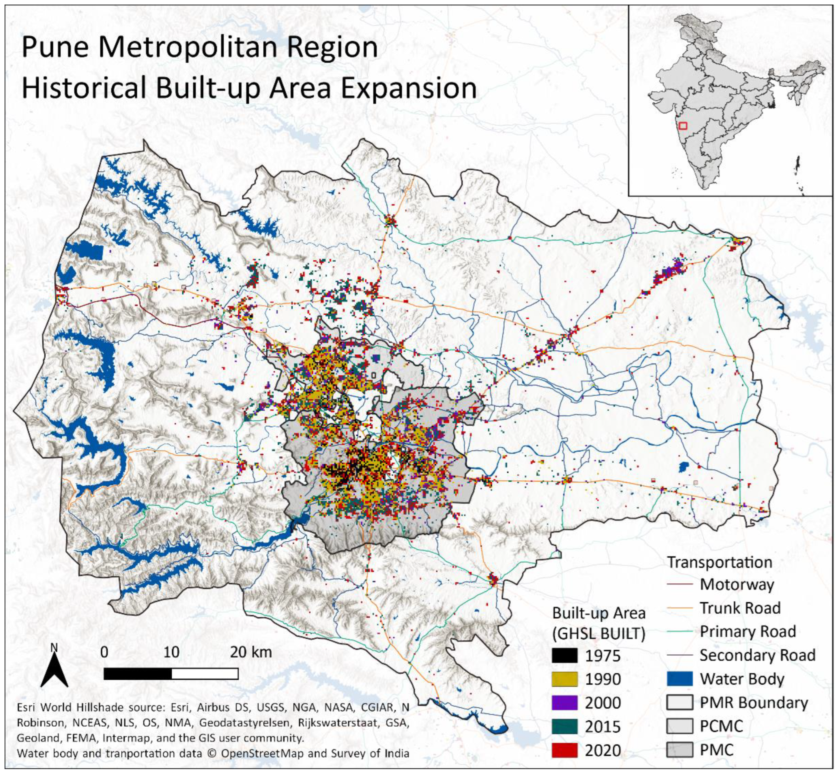
2.2. Study Site: Pune

Pune is located in the western part of Maharashtra, forming an urban-industrial corridor with Thane and Mumbai. We focus on the Pune Metropolitan Region (PMR), encompassing the Pune Municipal Corporation (PMC) and its northern twin city Pimpri Chinchwad (PCMC), as well as (parts of) 9 further subdistricts with 13 towns, over 800 villages, and large military cantonments [44]. Notwithstanding its image as a prosperous and livable city [45], Pune struggles with infrastructural deficits (insufficient water, energy, and transport systems) and institutions incapable of keeping up with the city’s rapid growth [46]. Between 22% and 32% of the PMC’s population live informally, many of whom have come to the city as domestic migrants [47,48]. The PMR has experienced a pronounced growth in population and built-up area over the last decades: the metropolitan population grew more than 3.5-fold from 2.5 million in 1975 to 9.13 million in 2020 [42,49] and built-up land by a factor of 9.3, corresponding to 323 km2 ([2,50] see Figure 2). The city’s expansion has largely been unregulated and increasingly dispersed in the past, particularly outside the corporations’ boundaries, where it consumed natural and agricultural land [35,51]. Garud and Rao [52] estimate that between 2014 and 2019, the PMR lost over 47 km2 of farmland to urbanization, mainly cropped with cereals, legumes, and vegetables. Like many Indian cities, Pune has experienced severe flood damage in the past. Due to the increasing share of an impervious surface in the city, Kumar and Dhorde [53] found significant increases in stormwater runoff and associated pluvial flood risk over the last decades. Moreover, riverine floods along Mula and Mutha have recently caused massive damage [54,55,56], affecting vulnerable populations groups most severely [57].

2.3. Future Scenario Estimation

2.3.1. Regionalization of Demographic and Economic Scenarios

Many studies have shown that the expansion of built-up areas is primarily driven by population and economic growth [10,11,58]. We hence base the future physical growth of the city on these two predictors. The globally available scenario portfolio Shared Socioeconomic Pathways (SSPs) is employed to define three different demographic and economic trajectories for Pune until the year 2050. We use three of the five available SSPs for our projections: SSP2 is treated as a business as usual (BAU) scenario, SSP1 as high-urbanization (HiUrb), and SSP3 as a low-urbanization (LoUrb) scenario.
Our Population projections are based on national SSP time series of the urban population provided by KC and Lutz [59] and Jiang and O’Neill [60]. These national projections are first regionalized to the state level alongside previous work conducted by KC et al. [61], and then to the PMR level, assuming proportionality among the three SSPs between national and state estimates and a fully urban population in the PMR. We update the SSPs’ base year to 2020 population numbers based on Schiavina et al.’s GHSL POP data [42].
Future economic projections are captured in the form of per capita district domestic product (DDPpc), again based on national SSP estimates [62]. A linear regression model is used to derive the PMR’s DDPpc estimates from national projections. The regression model is fitted using data from 1990/91 to 2014/15 on the Pune district (as a reasonable proxy for the PMR, where no DDPpc data are available) and national level. Both historical and future monetary values are adjusted for inflation to a constant 2010 Indian Rupee (INR2010) via the national consumer price index and the projections are corrected to the latest (2020) observed values [63]. Population and DDPpc are projected for each scenario in yearly time steps until 2050.

2.3.2. Estimating Future Built-Up Expansion via Beta Regression

The built-up fraction of a given region can be modeled as a constrained, monotonously growing function defined by the two predictors population density and DDPpc, typically following a sigmoid-shaped curve [58]. We apply a beta regression model with a logit link function to approximate this relationship. In the literature, beta regression models have been used to model various phenomena such as the fraction of plant cover in a habitat [64] (p. 340). To our knowledge, its application to built-up share is new. We use Ferrari and Cribari-Neto’s [65] parameterization of the beta function using the mean and precision parameters µ = p / p + q   and   φ = p + q , respectively:
f y ;   µ ,   φ = Γ φ Γ µ φ Γ 1 µ φ y µ φ 1 1 y 1 µ φ 1 ,     0 < y < 1
where 0 < µ < 1 and φ > 0. For our regression model, the mean μ of the response given observed covariates x is consequently:
g µ t = 1 k x t i β i
This follows the general structure of a multiple linear regression with β = β 1 β k T as the regression parameter vector and x t 1 x t k as the k observed covariates. To fit the unit interval (the share of built-up land can only range between 0 and 1), we apply a logit link function g · to the linear predictor.
For model fitting to Pune, 573 historical subdistrict-level observations of built-up and population density, as well as DDPpc, from Maharashtra and northern Karnataka are used. The approach of using cross-sectional data of the larger region, rather than a time series limited to the model region, is employed to reduce historical path dependency: the relationship of built-up area and population density/DDPpc of a neighboring, more urbanized city is likely to provide more accurate information on Pune’s growth than its own historical trajectory. The built-up area input is based on the Global Human Settlement Layer GHSL BUILT, derived from Landsat and Sentinel satellite imagery [2,50]. GHSL BUILT is resampled in GIS to the CA model resolution and to binary values (non-built-up/built-up; see Section 2.4). We use R’s glmmTMB package for model fitting (maximum likelihood) and prediction [66]. Several variations of the linear predictor were tested and compared via an analysis of variance (ANOVA, see Supplementary Materials). The linear predictor of the final regression model can be found in Equation (3). Both independent variables are log-transformed.
B u i l t u p n o r m = β 0 + β 1 log P O P n o r m + β 2 log D D P p c + ε
For the estimates of future built-up expansion for each of the three scenarios BAU, HiUrb, and LoUrb, we assume the irreversibility of urban land conversion [11,58], keeping built-up expansion stagnant in times of population and economic decline. Projections are further adjusted to the latest observed built-up extent and equipped with 95% confidence intervals.

2.4. Cellular Automaton–Built-Up Area Allocation

As the core of CitySCAPE, a cellular automaton (CA) allocates the total built-up area from the regression model on a grid of cells. The CA model can be run in calibration, validation, and future projection mode and is implemented in Java-based NetLogo [67].
CAs are found to approximate the actual development of a city reasonably well [21]. Arguably, they reflect how real-world decisions are made in cities—often individually, but influenced by numerous physical, economic, and social “landscapes” [68]. A highly popular example of an urban CA model is SLEUTH [68], where the urbanization of a cell is simulated through different growth types and its terrain steepness (slope) as a proxy for suitability, while the total growth rate is dynamically adapting. SLEUTH’s advantage, its simple structure, and limited data requirement also limits its applicability and accuracy, prompting numerous modifications, e.g., the inclusion of further physical, socio-economic, and political urbanization factors [69,70,71,72]. Our CA adopts and expands several of SLEUTH’s core components.
The CA’s model region is characterized by a two-dimensional regular grid of cells. Cell states (non-built-up/built-up) change in rounds of iteration, representing the time steps of one year. The cell state S i , j t + 1 is defined by its former state S i , j t , as well as neighborhood conditions ( Ω i , j t ), and transition rules ( T ), which determine the probability of a cell to urbanize (Equation (4); cf. [16]). A city’s growth pattern typically changes over time. For modeling, this requires the dynamic modification of parameters via self-modification (SM). The model is calibrated to reflect local characteristics using a set of suitability, growth, and self-modification parameters.
S i , j t + 1 = f S i , j t Ω i , j t T   S M
Initial cell states and neighborhood conditions are defined via GIS raster input data read into the model at the start.
As Table 1 and Figure 3 show, the input layers comprise the terrain’s slope, areas excluded from development (water bodies, protected natural areas, and military; Figure 3A), as well as the transportation infrastructure (roads, railway, and metro stations) and observed urban extent (both Figure 3B). Transportation and built-up layers contain information evolving over time and are therefore updated during model runs. For the case of Pune, the input data have a resolution of 7.5 × 7.5 arcsec (approx. 225 m × 225 m) cells, covering a space of approx. 130,000 cells.
Based on these inputs, the suitability of cells to be urbanized is calculated dynamically. To determine whether a cell is suitable to be built up in a given time step, the two factors slope and gravity, i.e., the distance to urban areas and transportation infrastructure, are used. While the slope is a standard variable in most urban CAs, CitySCAPE’s inclusion of a gravity layer—based on distance decay functions for each cell to urban areas and transportation (see Figure 3C)—is motivated by studies highlighting the importance of proximity effects on the urban form in growing (mega-) cities [72,79,80]. The weight of the two parameters, as well as the distance decay function’s form, is determined during calibration. With changing urban extents and transportation networks, the cell’s suitability is recalculated periodically, always containing a component of stochastic perturbation.
Once the suitable cells are identified, the total number of cells to be urbanized in the given time step, as defined a priori during scenario estimation, is placed on the map following four distinct growth types (see Figure 4): infill growth, i.e., the development of the areas within urban areas; urban sprawl, the spreading of the city at the fringe; ribbon development, the growth of the city along the transportation infrastructure; and scatter development, the spontaneous development of land in the periphery. These four types are slightly modified versions of SLEUTH’s growth rules. All types have been found in Pune’s historic development [51]. The number of cells allocated by each growth type is defined via growth parameters during calibration.
Self-modification is implemented by periodically altering the growth and suitability parameters. Studies paint a clear picture of decentralization, fragmentation, and increasing complexity of (mega-) cities associated with increasing size and maturity [81,82,83,84]. We use these observations to provide a simple self-modification module based on the two parameters form change and suitability change, which—in combination with the parameters of the current urban form—modify growth parameters every fifth time step. These change parameters are calibrated alongside the growth parameters.
The CA is calibrated via brute force, comparing the observed built-up area with multiple averaged Monte Carlo model runs. With calibration runs starting in 1975, three time steps are used for comparing observed and modeled expansion: 1990 (t = 14), 2000 (t = 24), and 2014 (t = 38). Suitability, growth, and self-modification parameters can take values between 0 and 100. We use a composite calibration metric across all time steps based on the product of R2 of mean slope, mean X-coordinate, and mean Y-coordinate, as well as the number of edges, and individual urban clusters. The metric is a variation of the Optimum SLEUTH Metric (OSM) developed by Dietzel and Clarke [85]. In addition, visual checks guide calibration by comparing modeled and observed urban forms in GIS for different parameter combinations. This is particularly relevant in case of similar OSM results among diverging parameter combinations during a calibration run. During calibration, a rigorous regime of parameter convergence is followed, in which the parameter space is repeatedly divided in half over six rounds. For proper model validation, runs on independent datasets are critical [21]. We use layers of observed urban expansion for 2015 and 2020 for a cell-by-cell comparison with single-run model results, as well as a spatial pattern analysis via mean slope, mean X-coordinate, mean Y-coordinate, the number of edges, and clusters (cf. [86]), and further accuracy-based validation approaches based on a contingency matrix (see Supplementary Materials). The validation of land use models has been the subject of debate for decades [87]. Simple crisp accuracy tests have limited the explanatory value in determining allocation disagreement due to their dependence on model size and urban complexity. Hence, we follow the METRONAMICA approach [88] and evaluate the results with Fuzzy Kappa and Fuzzy Kappa Simulation metric developed by van Vliet et al. [89] to assess the grades of similarity beyond slight disagreements (cf. [90] for a similar approach). A fuzzy similarity map yields cell values ranging from 0 (fully distinct) to 1 (fully identical). While Fuzzy Kappa compares the total urban extent including historical growth, Fuzzy Kappa Simulation is limited to newly urbanized cells within the validation period [91]. Cell values are calculated based on a distance decay function in a neighborhood of 16, and a halving distance of 8 cells, respectively.
Future simulations are generated by running the model from the latest observed point in time (2020) with calibrated parameters. CA models purposefully possess stochastic perturbation, leading to different results in every model run. We, therefore, generate both individual built-up maps to assess and visualize the urban shape as well as built-up probability maps in which Monte Carlo simulations generate average maps of multiple (e.g., 10 or 100) model runs. Cell values in probability maps close to 1 correspond to a high probability of urbanization, while values close to 0 represent cells unlikely to be built up in the future.

2.5. Dasymetric Mapping—Population Distribution over Built-Up Area

With dasymetric mapping as developed by Mennis [92], the population of an administrative area is distributed by using built-up density as ancillary data (cf. [41]). In CitySCAPE, dasymetric mapping is conducted in two steps: first, a population base map for the latest observed year (2020) is generated with input data on the village level. Then, projected future changes in the population on the PMR level are added/subtracted. The generation of a base map instead of directly using existing global population grids, such as GHSL POP, is optional but greatly increases consistency with existing census data [48] since it allows for a more fine-grained distinction between administrative units.
For preparation, CA’s 10-run built-up probability maps generated in 2.4, as well as the latest observed built-up and population data (GHSL BUILT and GHSL POP 2020), are resampled from 7.5 × 7.5 arcsec to 30 × 30 arcsec. The resulting cells are sorted into 160 urbanization classes defined by their share of built-up land between 0 (no built-up area) and 1 (fully built-up). The observed data are used to compute a population density fraction of each of the 160 urbanization classes. It indicates the relative difference in population density among the urbanization classes and is estimated individually for each subdistrict within the PMR via linear regression. For the 2020 base map, the total PMR population as derived in Section 2.3 is distributed across all villages/wards according to their share as per census. Via dasymetric mapping, each village’s/ward’s population is then distributed over its grid cells according to their urbanization class. For distributing the yearly population change of each urbanization scenario from 2021–2050 (including local shrinkage), the base map’s dasymetric mapping approach is slightly modified: to not constrain future flows between regions of the PMR, we use the PMR totals, not village/ward estimates as the input for the distribution. We further assume the population density fraction to remain constant in the future for each subdistrict. Importantly, this only relates to the relative difference in the population density of cells with a higher and lower built-up share—the actual density changes. A typical question in dasymetric mapping is how to deal with non-built-up cells. Remote sensing and the subsequent resampling of built-up land omit smaller, dispersed residential structures. In the model, we therefore assign a population density fraction to the non-built-up class as well. To reflect the different urbanization trajectories of the three scenarios (BAU, HiUrb, LoUrb), we discount this fraction to varying degrees in future projections (see Supplementary Materials). The dasymetric mapping model is implemented in Microsoft Excel/VBA. It ultimately generates a base year map as well as yearly estimates for each scenario of population totals per cell, and the population density in persons/km2.

2.6. Sustainability Assessments

Further GIS and statistical analyses are conducted on the built-up and population maps created in Section 2.4 and Section 2.5: changes in the spatial shape of the city are calculated using the established indices Mean Perimeter to Area Ratio (MPAR), Contrasting Edge Ratio (CER), and Patch Density (PD), respectively (cf. [83]). Population density, defined here as the number of people per square kilometer within an administrative area (in this case the PMR or PMC/PCMC), is calculated, as well as built-up area population density, i.e., the ratio of population and built-up area (cf. [93]). Furthermore, multiple single-run built-up maps are combined with a recent high-resolution land cover layer (WorldCover; [77]) to estimate land conversion between 2020 and 2050. For flood risk estimation, we combine both built-up probability maps and population density maps with official flood risk demarcations: in Pune, the most widely used flood levels are the blue and red flood lines corresponding to the “danger level” (25-year flood event) and “disaster level” (100-year flood event) [78]. Since these lines have repeatedly been surpassed in recent years and shown in simulations to be overly optimistic [94], we additionally create a 1 km corridor around the Mula and Mutha rivers of a potentially elevated food risk. Since the latter is not based on topographic and hydrological observations, it serves for illustration rather than an exact analysis. To estimate affectedness, we compute the area and number of affected people based on model outputs and cell overlap with the respective flood risk demarcations.

3. Results

3.1. Model Fitting and Calibration for Pune

In this section, we present selected results of parameter estimates and model performance for the case of the PMR. Further, goodness-of-fit tests are found in the Supplementary Materials. For the beta regression, the coefficient estimates, as well as standard error, z- and p-value are presented in Table 2. All coefficient estimates are highly significant (p < 0.001). For residual diagnostics, see Supplementary Materials.
The CA module calibration results are presented in Table 3: part A provides final parameter values, part B the R2 of the five calibration metrics and the total score. In terms of the validation results, over 10 validation runs, a mean Fuzzy Kappa of 0.96, and a mean Fuzzy Kappa Simulation of 0.55 were achieved for the PMR. For the landscape pattern validation, we compare multiple-run averages with the observed data. The location parameters mean slope, mean X-coordinate, and mean Y-coordinate, as well as the morphology parameter number of edges, show on average an agreement above 95% between the modeled and observed layers. The results and goodness-of-fit statistics of the linear regression in dasymetric mapping are found in the Supplementary Materials.

3.2. Model Results Pune

A general overview of the three urbanization scenarios is provided in Table 4 and Figure 5. In all cases, we find marked growth in terms of population, economy, and built-up land. Depending on the scenario, the population increases by 3.4 to 5.7 million by 2050. Notably, rural–urban migration as a potentially major growth engine [95] is not captured explicitly by the regionalized SSPS due to lacking data, suggesting conservative projections. The DDPpc more than doubles in LoUrb and almost quadruples in HiUrb. Demographic and economic development jointly drive Pune’s physical expansion, projecting an increase in the built-up area between 58% and 103%. Under BAU conditions, the beta regression model predicts 90 ± 30% growth, corresponding to the conversion of 325 ± 109 km2 of land (10.83 ± 4 km2 per year). For comparison: between 1990 and 2020, the urban land conversion was only 206 km2, i.e., 6.88 km2 per year. Population is the more influential driver of built-up growth, confirming previous findings for India [10]. Due to its steep increase, however, economic growth contributes significantly as well.
Pune’s physical shape will likely remain on its trajectory of rapid expansion and increasing fragmentation. Figure 6 shows the built-up probability for PMC and PCMC under BAU conditions. Future expansion can mainly be expected in Pune’s fringe area and along the transportation infrastructure. We see growth towards the north (shift in the center of gravity of around 1.5 km) and east (approx. 0.9 km shift), despite the dynamic development along the Pune–Mumbai corridor. In the south and southwest, the foothills of the Western Ghats create a less attractive topology for development, reflected in significantly lower growth. With regards to land conversion, 51% of the projected newly built-up land in 2050 (BAU scenario) takes place on formerly agricultural land, primarily found in the northwestern periphery (Figure 7). This corresponds to a loss of 167 km2 of arable land within the next 30 years. Additionally, 71 km2 of vegetated natural land (forest, shrub-, and grassland) are expected to be lost to construction, found in the city center as well as the Western Ghats. Both estimates are likely conservative due to the imperfect matching of 2020′s WorldCover and GHSL BUILT datasets (see category “Built-up (prev.)” in Figure 7). In general, we find that Pune’s complexity, discontiguity, and especially fragmentation continue to grow in the future. Consequently, MPAR and CER increase slightly by 2.3% and 3.4%, and PD almost triples in the BAU scenario, indicating a large number of small additional urban patches in the PMR.
In terms of population density, we see increases under all three scenarios throughout the PMR (see Figure 8). Peri-urban areas (the PMR outside PMC and PCMC) experience a moderate increase of 49% under BAU conditions from approximately 300 to 450 persons/km2. In contrast, the average population density of the PMC increases by 74% from 5600 to 9800 persons/km2. In the HiUrb scenario, the PMC’s density increase reaches 86%, and in LoUrb, 39%. When looking at the built-up area population density, the picture is different: within the PMC/PCMC, the built-up area population density remains constant at around 21,500 persons/km2 (BAU scenario), indicating that demographic and physical growth in the core city is balanced. In peri-urban areas, it declines from approximately 60,000 to 17,000 persons/km2, i.e., the built-up area grows faster than the population. Notably, the peri-urban built-up population density in 2020 is significantly higher than in the core city, owing to the underestimation of small residential structures in the remotely-sensed built-up data.
With regards to flood risk, we estimate the current and projected built-up area and the number of people within the three flood risk demarcations of the blue and red lines, as well as the 1 km corridor (yellow line). Satellite imagery confirms that the city has encroached into the riverbanks in the past, showing both informal and formal settlements within the red and blue flood lines. As Table 5 indicates, we estimate that 146,000 (blue line) and 193,000 (red line) people reside in the areas today already. If no effective development restrictions are implemented in the future, the built-up area and the number of residents are expected to increase significantly in all three flood risk demarcations (see detail of population map in Figure 9). Construction and population growth are higher in each of the three flood risk demarcations than the average of PMC and PCMC. Almost 0.9 million additional residents are projected to live within the yellow corridor in 2050, and approximately 95,000, and 30,000 within the red and blue flood lines, respectively.

4. Discussion

Our results show how global population scenarios can be translated into local trajectories of land-use change and population density. This is highly relevant in times of rapid urbanization, where cities search for sustainable and resilient development paths. The ex-ante definition of population and built-up totals via scenario downscaling and beta regression is more resource-intensive than simple CA models, where built-up demands are endogenously determined. It allows the user, however, to flexibly and transparently compare different future narratives across regions and scales, and it increases interoperability with other scenario-based models [11,16]. For instance, we find in our analysis that the local impacts of scenarios can deviate substantially from their global parents: while SSP1, the basis for our HiUrb scenario, is termed “Sustainability—the green road” and SSP3 “Regional rivalry—a rocky road” on a global level, we find HiUrb’s strong urbanization pressure to have the most severe impacts on the sustainability and resilience in the Pune Metropolitan Region.
The use of scenario corridors, rather than single predictions, reduces the risk of missing future trajectories. For Pune, differences among the three scenarios are significant: in only 30 years, the HiUrb scenario leads to 2.3 million more residents in the PMR than LoUrb. In any case, expected population growth is rapid, surpassing previous estimates: Hoornweg and Pope [96] projected the metropolitan population based on the UN’s World Urbanization Prospects to reach 10.9 million by 2050, which is even below our LoUrb estimation.
On the other hand, the breaking down of global scenarios to concrete manifestations in terms of land-use change and population distribution on the ground–provides actionable information for local planning: In Pune, the doubling of the built-up area in the next 30 years as expected by the HiUrb scenario, with BAU following closely, and the expected future densification of the population pose potentially serious challenges to the city’s sustainability and resilience. Three aspects illustrate this: (1) the increasingly concentrated resource demand in the city center, (2) developments on high flood-risk land, and (3) the loss of farmland in the fringe area.
(1)
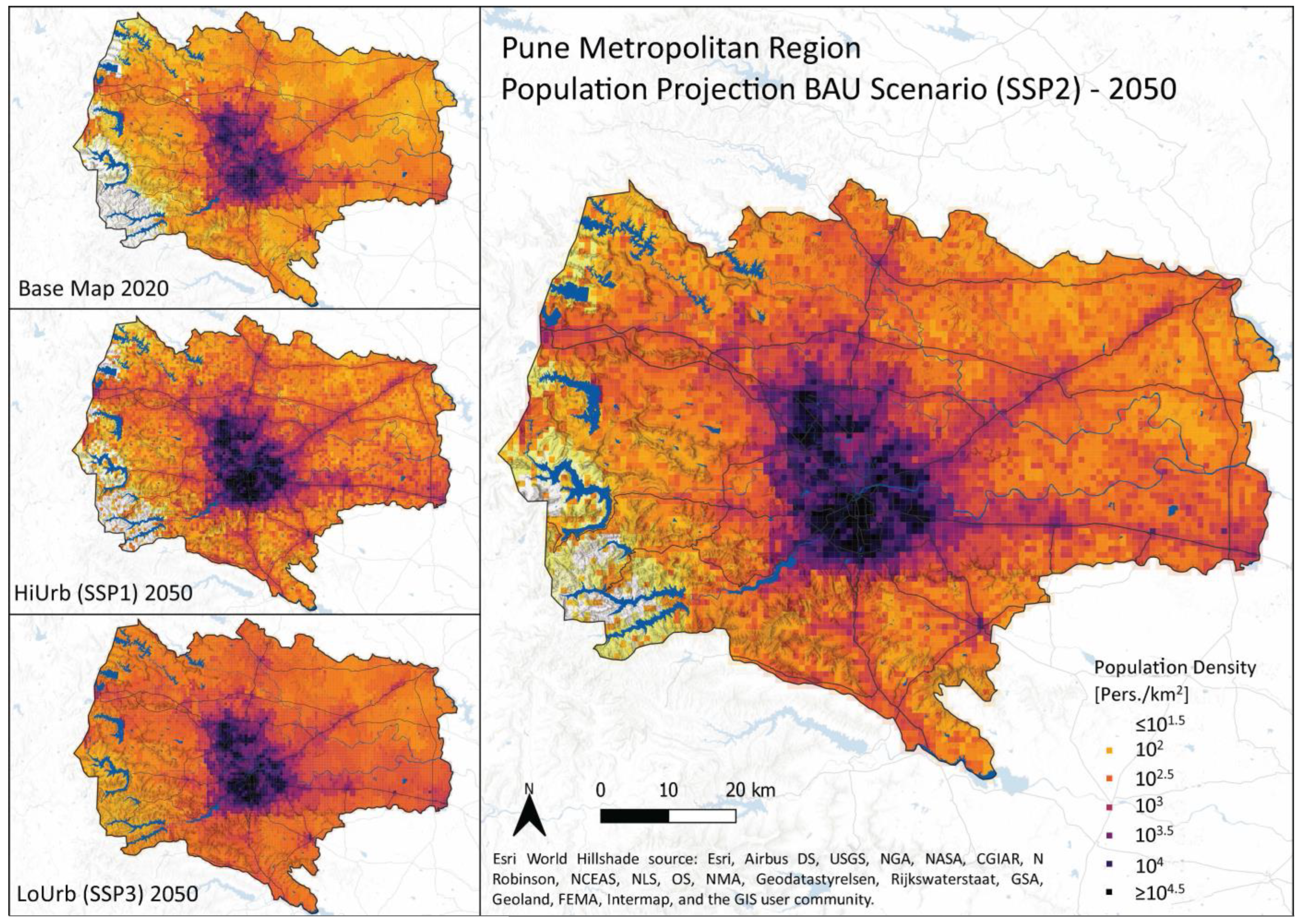
With up to 49,000 dwellers per km2, Pune’s urban core is already today extremely crowded. Our results show that its peak density will further increase, especially since the expected population growth will not distribute evenly across the metropolitan area but concentrate in the urban center and along the transportation infrastructure. In the BAU scenario, the maximum density reaches 60,000 persons/km2 by 2050 in PMC. Contrasting the population density with the built-up area population density, which does not increase, points to the need for adequate and comparable metrics. Overcrowding has been highlighted as a key challenge in Pune’s Food-Water-Energy nexus during co-creation workshops in 2019 and 2020: already today, water, electricity, and the transportation infrastructure are barely satisfying growing demands [97]. For example, the insufficient piped water network has led to the drilling of more than 100,000 borewells in the city, extracting approximately 113 million m3/year of groundwater, a fourth of the piped supply [98]. If the demand continues to outpace the municipal supply, a massive overuse of groundwater, as well as growing tanker water markets, can be expected.
(2)
Pune has suffered great losses during recent floods. The flood risk of a particular location depends on many factors and our analysis can only be a first approximation. We see, however, two trends potentially aggravating the situation: the significant inner-city surface sealing due to ongoing construction, and disproportionally active developments around the Mutha and Mula rivers, especially in the northern PMC. It should be noted that current or future policies to restrict development within flood-risk areas are not implemented in the model. Here, future work on the simulation of the effectiveness of different riverbank protection schemes, as well as the city’s controversial riverfront development plans, could yield valuable insights.
(3)
Over half of the land conversion in the BAU scenario is projected to take place on agricultural land. This is an even higher share than in the past and may exacerbate the adverse effects on local food security and rural livelihoods postulated by Garud and Rao [52]. From an ecological perspective, the sharply increasing fragmentation of the PMR’s landscape is particularly problematic due to the partitioning of habitats in the fringe area, reducing ecological connectivity [99].
Naturally, each of the model parts and their combination come with uncertainties and limitations. While the statistical tests attest good performance of beta regression and cellular automaton, the path dependencies inherent to dasymetric mapping that uses today’s relationship between the built-up area and population density fraction for future estimation should be kept in mind. Despite their limitations, however, population density maps add an entirely new dimension to urban growth projections, as our estimates of potentially flood-affected people illustrate. In any case, the scenario projections for 2050 should not be mistaken as predictions but as examples of possible futures.

5. Conclusions

The highly dynamic development of urban areas in many parts of the world requires long-term urbanization models that are based on established socio-economic scenarios, closely attuned to local conditions, and that include estimates of population distribution in addition to the built-up area. CitySCAPE fuses spatio-statistical approaches, cellular automata (CA), and dasymetric mapping to combine their strengths: the robust and comparable derivation of the future population and built-up demand, the spatially explicit mapping and of the built-up area via locally calibrated CA, and an idea where people will live in future via dasymetric mapping. To our knowledge, this has not been conducted previously. In Pune, we see how differently the future of a city can unravel depending on the overarching socio-economic trends. Our spatially explicit built-up and population analyses show that impacts are unevenly distributed across the metropolitan region and that a generally favorable scenario (HiUrb, SSP1) can have adverse impacts on the local level. The three urbanization challenges presented in this article serve as examples of potential fields for application of the model suite. Further work can deepen the analyses, e.g., by linking CitySCAPE with flood models, multi-agent systems, or spatially explicit groundwater, energy, and agricultural models for an integrated analysis of the urban Food-Water-Energy nexus. Efforts in this direction may include the simulation of sustainability effects of development plans and other interventions, an explicit inclusion of (climate) migration flows into population scenarios, a distinction between housing types (formal and informal), or the expansion of the CA by infrastructure layers such as a piped water network or electricity grid, and of course the application to other cities.
CitySCAPE is intended to be applied beyond academic users. The model development started in response to stakeholders pointing out the significant sustainability effects, particularly in terms of the Food-Water-Energy nexus, of Pune’s rapid urbanization in 2019. We hope that the limited coding knowledge required for its operation and the extensive documentation provided in the Supplementary Materials reduce uptake hurdles by practitioners. The model’s transferability to any urbanizing region and its compatibility with other simulation approaches allow for a broad range of applications. This may help cities to maneuver urbanization challenges by anticipating adverse effects and exploring the multiple opportunities it has to offer.

Supplementary Materials

All supporting information, including data, code, detailed model documentation, and further results, are provided on FigShare (https://doi.org/10.6084/m9.figshare.21524556) (accessed on 8 May 2023).

Author Contributions

Conceptualization, R.K. and C.J.A.K.; methodology and software, R.K.; calibration and validation, R.K.; formal analysis and investigation, R.K.; writing—original draft preparation, R.K.; writing—review and editing, R.K., S.K. and C.J.A.K.; visualization, R.K.; supervision, C.J.A.K. and S.K. All authors have read and agreed to the published version of the manuscript.

Funding

This work was conducted as part of the Belmont Forum Sustainable Urbanisation Global Initiative (SUGI)/Food–Water–Energy Nexus theme for which coordination was supported by the US National Science Foundation under grant ICER/EAR-1829999 to Stanford University. UFZ received funding from the Federal Ministry of Education and Research (BMBF) under grant number 033WU002. Any opinions, findings, conclusions, or recommendations expressed in this material do not necessarily reflect the views of the funding organizations.

Data Availability Statement

The data presented in this study are openly available on FigShare (https://doi.org/10.6084/m9.figshare.21524556) (accessed on 8 May 2023).

Acknowledgments

We would like to thank Jasmin Heilemann and Irene Garousi-Nejad for kindly sharing socio-economic and flood line data. The authors declare no competing interests.

Conflicts of Interest

The authors declare no conflict of interest.

References

  1. UN DESA. World Urbanization Prospects 2018: Highlights (ST/ESA/SER.A/421). 2019. Available online: https://population.un.org/wup/Publications/Files/WUP2018-Highlights.pdf (accessed on 5 September 2022).
  2. Corbane, C.; Florczyk, A.J.; Pesaresi, M.; Politis, P.; Syrris, V. GHS Built-Up Grid, Derived from Landsat, Multitemporal (1975–1990–2000–2014), R2018A. 2018. Available online: http://data.europa.eu/89h/jrc-ghsl-10007 (accessed on 10 June 2022).
  3. Lwasa, S.; Seto, K.C.; Bai, X.; Blanco, H.; Gurney, K.R.; Kilkiş, S.; Lucon, O.; Murakami, J.; Pan, J.; Sharifi, A.; et al. Urban systems and other settlements. In Climate Change 2022: Mitigation of Climate Change. Contribution of Working Group III to the Sixth Assessment Report of the Intergovernmental Panel on Climate Change; IPCC, Ed.; Cambridge University Press: Cambridge, UK; New York, NY, USA, 2022. [Google Scholar]
  4. IPBES. Global Assessment Report on Biodiversity and Ecosystem Services of the Intergovernmental Science-Policy Platform on Biodiversity and Ecosystem Services; Brondizio, E.S., Settele, J., Díaz, S., Ngo, H.T., Eds.; IPBES Secretariat: Bonn, Germany, 2019. [Google Scholar]
  5. Güneralp, B.; Reba, M.; Hales, B.U.; Wentz, E.A.; Seto, K.C. Trends in urban land expansion, density, and land transitions from 1970 to 2010: A global synthesis. Environ. Res. Lett. 2020, 15, 44015. [Google Scholar] [CrossRef]
  6. Follmann, A.; Willkomm, M.; Dannenberg, P. As the city grows, what do farmers do? A systematic review of urban and peri-urban agriculture under rapid urban growth across the Global South. Landsc. Urban Plan. 2021, 215, 104186. [Google Scholar] [CrossRef]
  7. Cao, W.; Zhou, Y.; Güneralp, B.; Li, X.; Zhao, K.; Zhang, H. Increasing global urban exposure to flooding: An analysis of long-term annual dynamics. Sci. Total Environ. 2022, 817, 153012. [Google Scholar] [CrossRef] [PubMed]
  8. Dodman, D.; Hayward, B.; Pelling, M.; Broto, V.C.; Chow, W.; Chu, E.; Dawson, R.; Khirfan, L.; McPhearson, T.; Prakash, A.; et al. Cities, Settlements and Key Infrastructure. In Impacts, Adaptation, and Vulnerability. Contribution of Working Group II to the Sixth Assessment Report of the Intergovernmental Panel on Climate Change; IPCC, Ed.; Cambridge University Press: Cambridge, UK; New York, NY, USA, 2022. [Google Scholar]
  9. Avashia, V.; Garg, A. Implications of land use transitions and climate change on local flooding in urban areas: An assessment of 42 Indian cities. Land Use Policy 2020, 95, 104571. [Google Scholar] [CrossRef]
  10. Seto, K.C.; Güneralp, B.; Hutyra, L.R. Global forecasts of urban expansion to 2030 and direct impacts on biodiversity and carbon pools. Proc. Natl. Acad. Sci. USA 2012, 109, 16083–16088. [Google Scholar] [CrossRef] [Green Version]
  11. Chen, G.; Li, X.; Liu, X.; Chen, Y.; Liang, X.; Leng, J.; Xu, X.; Liao, W.; Qiu, Y.; Wu, Q.; et al. Global projections of future urban land expansion under shared socioeconomic pathways. Nat. Commun. 2020, 11, 537. [Google Scholar] [CrossRef] [Green Version]
  12. O’Neill, B.C.; Kriegler, E.; Ebi, K.L.; Kemp-Benedict, E.; Riahi, K.; Rothman, D.S.; van Ruijven, B.J.; van Vuuren, D.P.; Birkmann, J.; Kok, K.; et al. The roads ahead: Narratives for shared socioeconomic pathways describing world futures in the 21st century. Glob. Environ. Change 2017, 42, 169–180. [Google Scholar] [CrossRef] [Green Version]
  13. Triantakonstantis, D.; Mountrakis, G. Urban Growth Prediction: A Review of Computational Models and Human Perceptions. J. Geogr. Inf. Syst. 2012, 4, 555–587. [Google Scholar] [CrossRef] [Green Version]
  14. Musa, S.I.; Hashim, M.; Reba, M. A review of geospatial-based urban growth models and modelling initiatives. Geocarto Int. 2017, 32, 813–833. [Google Scholar] [CrossRef]
  15. Kim, Y.; Newman, G.; Güneralp, B. A Review of Driving Factors, Scenarios, and Topics in Urban Land Change Models. Land 2020, 9, 246. [Google Scholar] [CrossRef]
  16. Li, X.; Gong, P. Urban growth models: Progress and perspective. Sci. Bull. 2016, 61, 1637–1650. [Google Scholar] [CrossRef]
  17. Tong, X.; Feng, Y. A review of assessment methods for cellular automata models of land-use change and urban growth. Int. J. Geogr. Inf. Sci. 2020, 34, 866–898. [Google Scholar] [CrossRef]
  18. Chang, N.-B.; Hossain, U.; Valencia, A.; Qiu, J.; Kapucu, N. The role of food-energy-water nexus analyses in urban growth models for urban sustainability: A review of synergistic framework. Sustain. Cities Soc. 2020, 63, 102486. [Google Scholar] [CrossRef]
  19. Von Neumann, J.; Burks, A.W. Theory of Self-Reproducing Automata; University of Illinois Press: Urbana, IL, USA, 1966. [Google Scholar]
  20. Tobler, W.R. A Computer Movie Simulating Urban Growth in the Detroit Region. Econ. Geogr. 1970, 46, 234–240. [Google Scholar] [CrossRef]
  21. Liu, Y.; Batty, M.; Wang, S.; Corcoran, J. Modelling urban change with cellular automata: Contemporary issues and future research directions. Prog. Hum. Geogr. 2019, 45, 030913251989530. [Google Scholar] [CrossRef]
  22. Verburg, P.H.; Soepboer, W.; Veldkamp, A.; Limpiada, R.; Espaldon, V.; Mastura, S.S.A. Modeling the spatial dynamics of regional land use: The CLUE-S model. Environ. Manag. 2002, 30, 391–405. [Google Scholar] [CrossRef]
  23. Mendbayar, O.; Badarifu; Ranatunga, T.; Onishi, T.; Hiramatsu, K. Cellular Automata Modelling Approach for Urban Growth. Rev. Agric. Sci. 2018, 6, 93–104. [Google Scholar] [CrossRef] [Green Version]
  24. Yadav, P.; Deshpande, S.S.; Ladha, S.; Curry, E. Computational Model for Urban Growth Using Socioeconomic Latent Parameters. In ECML PKDD 2018 Workshops: Nemesis 2018, UrbReas 2018, SoGood 2018, IWAISe 2018, and Green Data Mining 2018, Dublin, Ireland, 10–14 September 2018; Springer: Cham, Switzerland, 2019. [Google Scholar] [CrossRef]
  25. Ghosh, P.; Mukhopadhyay, A.; Chanda, A.; Mondal, P.; Akhand, A.; Mukherjee, S.; Nayak, S.K.; Ghosh, S.; Mitra, D.; Ghosh, T.; et al. Application of Cellular automata and Markov-chain model in geospatial environmental modeling—A review. Remote Sens. Appl. Soc. Environ. 2017, 5, 64–77. [Google Scholar] [CrossRef]
  26. Loibl, W.; Tötzer, T. Modeling growth and densification processes in suburban regions—Simulation of landscape transition with spatial agents. Environ. Model. Softw. 2003, 18, 553–563. [Google Scholar] [CrossRef]
  27. Mustafa, A.; Cools, M.; Saadi, I.; Teller, J. Coupling agent-based, cellular automata and logistic regression into a hybrid urban expansion model (HUEM). Land Use Policy 2017, 69, 529–540. [Google Scholar] [CrossRef] [Green Version]
  28. Liu, Y.; Kong, X.; Liu, Y.; Chen, Y. Simulating the conversion of rural settlements to town land based on multi-agent systems and cellular automata. PLoS ONE 2013, 8, e79300. [Google Scholar] [CrossRef]
  29. Kamusoko, C.; Gamba, J. Simulating Urban Growth Using a Random Forest-Cellular Automata (RF-CA) Model. ISPRS Int. J. Geo-Inf. 2015, 4, 447–470. [Google Scholar] [CrossRef] [Green Version]
  30. Thapa, R.B.; Murayama, Y. Scenario based urban growth allocation in Kathmandu Valley, Nepal. Landsc. Urban Plan. 2012, 105, 140–148. [Google Scholar] [CrossRef]
  31. Zhang, Y.; Liu, X.; Chen, G.; Hu, G. Simulation of urban expansion based on cellular automata and maximum entropy model. Sci. China Earth Sci. 2020, 63, 701–712. [Google Scholar] [CrossRef]
  32. Chaudhuri, G.; Clarke, K.C. Modeling an Indian megalopolis– A case study on adapting SLEUTH urban growth model. Comput. Environ. Urban Syst. 2019, 77, 101358. [Google Scholar] [CrossRef] [Green Version]
  33. Guan, C.; Rowe, P.G. Should big cities grow? Scenario-based cellular automata urban growth modeling and policy applications. J. Urban Manag. 2016, 5, 65–78. [Google Scholar] [CrossRef]
  34. Jantz, C.A.; Goetz, S.J.; Shelley, M.K. Using the Sleuth Urban Growth Model to Simulate the Impacts of Future Policy Scenarios on Urban Land Use in the Baltimore-Washington Metropolitan Area. Environ. Plan. B Plan. Des. 2004, 31, 251–271. [Google Scholar] [CrossRef]
  35. Kantakumar, L.N.; Kumar, S.; Schneider, K. SUSM: A scenario-based urban growth simulation model using remote sensing data. Eur. J. Remote Sens. 2019, 12, 26–41. [Google Scholar] [CrossRef] [Green Version]
  36. Hasan, S.; Deng, X.; Li, Z.; Chen, D. Projections of Future Land Use in Bangladesh under the Background of Baseline, Ecological Protection and Economic Development. Sustainability 2017, 9, 505. [Google Scholar] [CrossRef] [Green Version]
  37. Kuang, W. Simulating dynamic urban expansion at regional scale in Beijing-Tianjin-Tangshan Metropolitan Area. J. Geogr. Sci. 2011, 21, 317–330. [Google Scholar] [CrossRef]
  38. Zhang, D.; Huang, Q.; He, C.; Wu, J. Impacts of urban expansion on ecosystem services in the Beijing-Tianjin-Hebei urban agglomeration, China: A scenario analysis based on the Shared Socioeconomic Pathways. Resour. Conserv. Recycl. 2017, 125, 115–130. [Google Scholar] [CrossRef]
  39. Sinha, P.; Gaughan, A.E.; Stevens, F.R.; Nieves, J.J.; Sorichetta, A.; Tatem, A.J. Assessing the spatial sensitivity of a random forest model: Application in gridded population modeling. Comput. Environ. Urban Syst. 2019, 75, 132–145. [Google Scholar] [CrossRef]
  40. Dobson, J.E. LandScan: A Global Population Database for Estimating Populations at Risk. Photogramm. Eng. Remote Sens. 2000, 66, 849–857. [Google Scholar]
  41. Wardrop, N.A.; Jochem, W.C.; Bird, T.J.; Chamberlain, H.R.; Clarke, D.; Kerr, D.; Bengtsson, L.; Juran, S.; Seaman, V.; Tatem, A.J. Spatially disaggregated population estimates in the absence of national population and housing census data. Proc. Natl. Acad. Sci. USA 2018, 115, 3529–3537. [Google Scholar] [CrossRef] [PubMed] [Green Version]
  42. Schiavina, M.; Freire, S.; MacManus, K. GHS-POP R2022A: GHS Population Grid Multitemporal (1975–2030). 2022. Available online: https://ghsl.jrc.ec.europa.eu/datasets.php#inline-nav-ghs_pop2022 (accessed on 2 August 2022).
  43. Koomen, E.; van Bemmel, M.S.; van Huijstee, J.; Andrée, B.; Ferdinand, P.A.; van Rijn, F. An integrated global model of local urban development and population change. Comput. Environ. Urban Syst. 2023, 100, 101935. [Google Scholar] [CrossRef]
  44. PMRDA. Pune Metropolitan Region Development Authority: Background. Available online: http://www.pmrda.gov.in/pmrda_background (accessed on 3 November 2022).
  45. MoHUA. City Rankings 2020: Ease of Living. Available online: https://eol.smartcities.gov.in/dashboard (accessed on 1 February 2023).
  46. Butsch, C.; Kumar, S.; Wagner, P.D.; Kroll, M.; Kantakumar, L.N.; Bharucha, E.; Schneider, K.; Kraas, F. Growing ‘Smart’?: Urbanization Processes in the Pune Urban Agglomeration. Sustainability 2017, 9, 2335. [Google Scholar] [CrossRef] [Green Version]
  47. MASHAL. The Slum Atlas: Publications. 2011. Available online: https://www.mashalngo.org/Slum-Atlas.html (accessed on 15 February 2022).
  48. GOI. Census—Data and Resource. Available online: https://censusindia.gov.in/census.website (accessed on 30 November 2022).
  49. Schiavina, M.; Freire, S.; MacManus, K. GHS-POP R2019A—Population Grid Multitemporal (1975–1990–2000–2015). 2019. Available online: http://data.europa.eu/89h/0c6b9751-a71f-4062-830b-43c9f432370f (accessed on 1 May 2021).
  50. Pesaresi, M.; Politis, P. GHS Built-Up Surface Grid: Derived from Sentinel2 Composite and Landsat, Multitemporal (1975–2030). 2022. Available online: https://ghsl.jrc.ec.europa.eu/datasets.php#inline-nav-ghs_buS2022 (accessed on 2 August 2022).
  51. Kantakumar, L.N.; Kumar, S.; Schneider, K. Spatiotemporal urban expansion in Pune metropolis, India using remote sensing. Habitat Int. 2016, 51, 11–22. [Google Scholar] [CrossRef]
  52. Garud, A.; Rao, B. Understanding the Implications of the Loss of Peri-Urban Arable Land—A Case of Pune Metropolitan Region. In Urban Science and Engineering: Proceedings of ICUSE 2020, 1st ed.; Jana, A., Banerji, P., Eds.; Springer: Singapore, 2021; pp. 433–445. ISBN 978-981-33-4113-5. [Google Scholar]
  53. Kumar, K.; Dhorde, A. Impact of Land use Land cover change on Storm Runoff Generation: A case study of suburban catchments of Pune, Maharashtra, India. Environ. Dev. Sustain. 2021, 23, 4559–4572. [Google Scholar] [CrossRef]
  54. TNN. How Pune went under water, vehicles washed away in floods. The Times of India, 27 September 2019. Available online: https://timesofindia.indiatimes.com/city/pune/how-pune-went-under-water-vehicles-washed-away-in-floods/articleshow/71322737.cms(accessed on 12 September 2022).
  55. Deshpande, S.; Wani, K.; Deodhar, A.; Gole, S.; Nulkar, G.; Gabale, S.; Shitole, T.; Kulkarni, H.; Bhagwat, M. Pune City Floods: Causes, Analysis and Mitigation Measures. 2021. Available online: https://www.researchgate.net/publication/353656111_Pune_City_Floods_Causes_Analysis_and_Mitigation_measures (accessed on 9 December 2022).
  56. Mundhe, N. Multi-Criteria Decision Making for Vulnerability Mapping of Flood Hazard: A Case Study of Pune City. J. Geogr. Stud. 2018, 2, 41–52. [Google Scholar] [CrossRef] [Green Version]
  57. Link, A.-C.; Zhu, Y.; Karutz, R. Quantification of Resilience Considering Different Migration Biographies: A Case Study of Pune, India. Land 2021, 10, 1134. [Google Scholar] [CrossRef]
  58. Li, X.; Zhou, Y.; Eom, J.; Yu, S.; Asrar, G.R. Projecting Global Urban Area Growth Through 2100 Based on Historical Time Series Data and Future Shared Socioeconomic Pathways. Earth’s Future 2019, 7, 351–362. [Google Scholar] [CrossRef] [Green Version]
  59. KC, S.; Lutz, W. The human core of the shared socioeconomic pathways: Population scenarios by age, sex and level of education for all countries to 2100. Glob. Environ. Change 2017, 42, 181–192. [Google Scholar] [CrossRef] [Green Version]
  60. Jiang, L.; O’Neill, B.C. Global urbanization projections for the Shared Socioeconomic Pathways. Glob. Environ. Change 2017, 42, 193–199. [Google Scholar] [CrossRef] [Green Version]
  61. KC, S.; Wurzer, M.; Speringer, M.; Lutz, W. Future population and human capital in heterogeneous India. Proc. Natl. Acad. Sci. USA 2018, 115, 8328–8333. [Google Scholar] [CrossRef] [PubMed] [Green Version]
  62. Crespo Cuaresma, J. Income projections for climate change research: A framework based on human capital dynamics. Glob. Environ. Change 2017, 42, 226–236. [Google Scholar] [CrossRef] [Green Version]
  63. World Bank. GDP per Capita (Constant 2010 US$)—India. Available online: https://data.worldbank.org/indicator/NY.GDP.PCAP.KD?locations=IN&most_r (accessed on 1 February 2022).
  64. Fox, G.A.; Negrete-Yankelevich, S.; Sosa, V.J. (Eds.) Ecological Statistics: Contemporary Theory and Application; Oxford University Press: Oxford, UK, 2015; ISBN 9780199672547. [Google Scholar]
  65. Ferrari, S.; Cribari-Neto, F. Beta Regression for Modelling Rates and Proportions. J. Appl. Stat. 2004, 31, 799–815. [Google Scholar] [CrossRef]
  66. Bolker, B. Getting Started with the glmmTMB Package. 2021. Available online: https://cran.r-project.org/web/packages/glmmTMB/vignettes/glmmTMB.pdf (accessed on 21 February 2022).
  67. Wilensky, U. NetLogo; Center for Connected Learning and Computer-Based Modeling, Northwestern University: Evanston, IL, USA, 1999. [Google Scholar]
  68. Clarke, K.C.; Hoppen, S.; Gaydos, L.J. A self-modifying cellular automaton model of historical urbanization in the San Francisco Bay area. Environ. Plan. B Plan. Des. 1997, 24, 247–261. [Google Scholar] [CrossRef] [Green Version]
  69. Li, F.; Wang, L.; Chen, Z.; Clarke, K.C.; Li, M.; Jiang, P. Extending the SLEUTH model to integrate habitat quality into urban growth simulation. J. Environ. Manag. 2018, 217, 486–498. [Google Scholar] [CrossRef] [Green Version]
  70. Saxena, A.; Jat, M.K.; Clarke, K.C. Development of SLEUTH-Density for the simulation of built-up land density. Comput. Environ. Urban Syst. 2021, 86, 101586. [Google Scholar] [CrossRef]
  71. Chaudhuri, G.; Clarke, K.C. The SLEUTH Land Use Change Model: A Review. Int. J. Environ. Resour. Res. 2013, 1, 88–104. [Google Scholar]
  72. Liu, D.; Clarke, K.C.; Chen, N. Integrating spatial nonstationarity into SLEUTH for urban growth modeling: A case study in the Wuhan metropolitan area. Comput. Environ. Urban Syst. 2020, 84, 101545. [Google Scholar] [CrossRef]
  73. NRSC; ISRO. Technical Methodology for Countrywide DEM and Ortho Product Generation for India Using Cartosat-1 Stereo Data: Version 1. 2013. Available online: https://bhuvan-app3.nrsc.gov.in/data/download/tools/document/SISDP-DEM-GENERATION-BHUVAN.pdf (accessed on 1 November 2020).
  74. UNEP-WCMC; IUCN. Protected Planet: WDPA—The World Database on Protected Areas; UNEP-WCMC: Cambridge, UK; IUCN: Cambridge, UK, 2020. [Google Scholar]
  75. OpenStreetMap. OSM Data India; Geofabrik: Karlsruhe, Germany, 2020. [Google Scholar]
  76. SOI. Topo Sheets Maharashtra [Various Years]; Survey of India: Dehradun, India, 2019. [Google Scholar]
  77. Zanaga, D.; van de Kerchove, R.; de Keersmaecker, W.; Souverijns, N.; Brockmann, C.; Quast, R.; Wevers, J.; Grosu, A.; Paccini, A.; Vergnaud, S.; et al. ESA World Cover: 10 m 2020 v100; ESA: Paris, France, 2021. [Google Scholar] [CrossRef]
  78. GoM WRD. Flood Line Marking Maps. Available online: http://www.punefloodcontrol.com/maps.html (accessed on 10 May 2022).
  79. Kantakumar, L.N.; Kumar, S.; Schneider, K. What drives urban growth in Pune? A logistic regression and relative importance analysis perspective. Sustain. Cities Soc. 2020, 60, 102269. [Google Scholar] [CrossRef]
  80. Tripathy, P.; Kumar, A. Monitoring and modelling spatio-temporal urban growth of Delhi using Cellular Automata and geoinformatics. Cities 2019, 90, 52–63. [Google Scholar] [CrossRef]
  81. Zhou, C.; Ye, C. Features and causes of urban spatial growth in Chinese metropolises. Acta Geogr. Sin. 2013, 68, 728–738. [Google Scholar]
  82. Jia, Y.; Tang, L.; Xu, M.; Yang, X. Landscape pattern indices for evaluating urban spatial morphology—A case study of Chinese cities. Ecol. Indic. 2019, 99, 27–37. [Google Scholar] [CrossRef]
  83. Zheng, D.; Zhang, G.; Shan, H.; Tu, Q.; Wu, H.; Li, S. Spatio-Temporal Evolution of Urban Morphology in the Yangtze River Middle Reaches Megalopolis, China. Sustainability 2020, 12, 1738. [Google Scholar] [CrossRef] [Green Version]
  84. Ramachandra, T.V.; Bharath, H.; Sreekantha, S. Spatial Metrics based Landscape Structure and Dynamics Assessment for an emerging Indian Megalopolis. Int. J. Adv. Res. Artif. Intell. 2012, 1, 48–57. [Google Scholar] [CrossRef] [Green Version]
  85. Dietzel, C.; Clarke, K.C. Toward Optimal Calibration of the SLEUTH Land Use Change Model. Trans. GIS 2007, 11, 29–45. [Google Scholar] [CrossRef]
  86. Camacho Olmedo, M.T.; Pontius, R.G.; Paegelow, M.; Mas, J.-F. Comparison of simulation models in terms of quantity and allocation of land change. Environ. Model. Softw. 2015, 69, 214–221. [Google Scholar] [CrossRef] [Green Version]
  87. Pontius, R.G.; Millones, M. Death to Kappa: Birth of quantity disagreement and allocation disagreement for accuracy assessment. Int. J. Remote Sens. 2011, 32, 4407–4429. [Google Scholar] [CrossRef]
  88. Van Delden, H.; Escudero, J.C.; Uljee, I.; Engelen, G. METRONAMICA: A Dynamic Spatial Land Use Model Applied to Vitoria-Gasteiz: Virtual Seminar of the Miles Project; Environmental Studies Centre: Vitoria-Gasteiz, 2005. [Google Scholar]
  89. Van Vliet, J.; Bregt, A.K.; Hagen-Zanker, A. Revisiting Kappa to account for change in the accuracy assessment of land-use change models. Ecol. Model. 2011, 222, 1367–1375. [Google Scholar] [CrossRef]
  90. Lauf, S.; Haase, D.; Hostert, P.; Lakes, T.; Kleinschmit, B. Uncovering land-use dynamics driven by human decision-making—A combined model approach using cellular automata and system dynamics. Environ. Model. Softw. 2012, 27–28, 71–82. [Google Scholar] [CrossRef]
  91. RIKS BV. Map Comparison Kit 3: User Manual, Maastricht. 2013. Available online: https://www.dropbox.com/s/94vbcq46xuo10hh/MCK_Reader.pdf (accessed on 16 May 2022).
  92. Mennis, J. Generating Surface Models of Population Using Dasymetric Mapping. Prof. Geogr. 2003, 55, 31–42. [Google Scholar] [CrossRef]
  93. Angel, S.; Blei, A.M.; Parent, J.; Lamson-Hall, P.; Sánchez, N.G.; Civco, D.L.; Lei, R.Q.; Thom, K. Atlas of Urban Expansion. The 2016 Edition: Volume 1: Areas and Densities; New York University: New York, NY, USA; UN-Habitat: Nairobi, Kenya; Lincoln Institute of Land Policy: Cambridge, MA, USA, 2016; Available online: https://www.lincolninst.edu/sites/default/files/pubfiles/atlas-of-urban-expansion-2016-volume-1-full.pdf (accessed on 24 January 2023).
  94. Chate, S.J.; Nimbalkar, P.T. Development of Flood Routing Model Using Hec-Ras Software for Mutha River in Pune City. Int. J. Eng. Adv. Technol. 2019, 8, 2302–2307. [Google Scholar]
  95. Karutz, R.; Kabisch, S. Exploring the Relationship Between Droughts and Rural-to-urban Mobility—A Mixed-Methods Approach for Pune, India. Front. Clim. 2023, 5. [Google Scholar] [CrossRef]
  96. Hoornweg, D.; Pope, K. Population predictions for the world’s largest cities in the 21st century. Environ. Urban. 2017, 29, 195–216. [Google Scholar] [CrossRef] [Green Version]
  97. Karutz, R.; Omann, I.; Gorelick, S.M.; Klassert, C.J.A.; Zozmann, H.; Zhu, Y.; Kabisch, S.; Kindler, A.; Figueroa, A.J.; Wang, A.; et al. Capturing Stakeholders’ Challenges of the Food–Water–Energy Nexus—A Participatory Approach for Pune and the Bhima Basin, India. Sustainability 2022, 14, 5323. [Google Scholar] [CrossRef]
  98. Kulkarni, H.; Bhagwat, M.; Kale, V.; Aslekar, U. Pune’s Aquifers: Some Early Insights from a Strategic Hydrogeological Appraisal; Advanced Center for Water Resouces Development and Management: Pune, India, 2019; Available online: https://www.researchgate.net/publication/335976478_PUNE%27S_AQUIFERS_Some_Early_Insights_From_A_Strategic_Hydrogeological_Appraisal?channel=doi&linkId=5d885b30458515cbd1b3ae25&showFulltext=true (accessed on 9 December 2022).
  99. Dupras, J.; Marull, J.; Parcerisas, L.; Coll, F.; Gonzalez, A.; Girard, M.; Tello, E. The impacts of urban sprawl on ecological connectivity in the Montreal Metropolitan Region. Environ. Sci. Policy 2016, 58, 61–73. [Google Scholar] [CrossRef] [Green Version]
Figure 1. Overview of the CitySCAPE Model Suite. Grey-shaded boxes represent the three main model parts; small boxes refer to model outputs.
Land 12 01051 g001
Figure 2. Historical expansion of the built-up area in PMR between 1975 and 2020. Own illustration based on GHSL BUILT [2,50].
Land 12 01051 g002
Figure 3. Building the model landscape, here for PMR and the year 2020: (A): physical properties (slope, excluded areas); (B): transportation infrastructure (roads, railway, and metro stations) and observed urban extent (“seed layer”); and (C): gravity to urban areas and transportation infrastructure.
Land 12 01051 g003
Figure 4. Schematic illustration of the four growth types (clockwise) with the hypothetical shape of Pune assuming the city grew only by this type from 1975 to 2014. (A): Infill growth (red), (B): sprawl growth (dark blue), (C): ribbon growth (blue), and (D): scattered growth (purple).
Land 12 01051 g004
Figure 5. (Left) Historical population development and future projections for PMR, in millions for HiUrb, BAU, and LoUrb scenario, based on downscaled SSP 1–3. (Right) Historical development and future projections of built-up area in km2 for PMR. Exemplary standard errors are indicated in hatched blue for the BAU scenario (SSP2).
Land 12 01051 g005
Figure 6. Conversion probability of cells in PMC and PCMC until 2050. BAU Scenario (SSP 2).
Land 12 01051 g006
Figure 7. Exemplary land conversion between 2020 and 2050 for BAU scenario in PMR. Detail A shows the high expected tree cover loss in the city center. Detail B shows that in the periphery, especially towards the northwest, agricultural land is expected to be lost (see also detail B). Chart in the bottom right: mean conversion over 10 model iterations. Source land cover: WorldCover by Zanaga et al. [77].
Land 12 01051 g007
Figure 8. Population distribution in PMR in 2020 (upper left corner), and 2050 for BAU (large map), HiUrb (center left), and LoUrb (bottom left). For better visibility, color increments relate to the log scale. Estimated via dasymetric mapping based on CitySCAPE model outputs and data by Pesaresi and Politis [50], Schiavina et al. [42], and GOI [48].
Land 12 01051 g008
Figure 9. Flood risk map: population density under BAU scenario (SSP2) in 2050 and blue, red, and yellow (1 km corridor) flood lines.
Land 12 01051 g009
Table 1. Spatial model input data. All spatial data layers are reprojected to EPSG 4326 and rasterized in model resolution. For further details, see Supplementary Materials.
DataDescriptionSource
Slope layerHill slope (%) derived from Cartosat DEM[73]
Exclusion layerAreas excluded from urbanization. Defined by OpenStreetMap’s land-cover/land-use classes water body and military, as well as protected areas as per the IUCN database.[74,75]
Transportation layerHistorical and current road and railroad network, as well as major infrastructure projects under construction (Pune metro, PMR ring road), based on digitized/geo-located SOI Toposheets, OpenStreetMap, and Planning documents. Years: 1975, 1990, 2000, 2030[75,76]
Observed urban extentMulti-temporal raster layer of built-up area. Global Human Settlement Layer (GHSL BUILT). Years: 1975, 1990, 2000, 2014, 2015, 2020[2,50]
Population distributionSpatially distributed population derived from Global Human Settlement Population Layer (GHSL POP) 2020.[42]
Census dataAdministrative boundaries within the PMR on village/ward level and associated census data.[48]
Land coverLand cover base map for calculation of urban land conversion: ESA WorldCover[77]
Flood linesDigitized/geo-located blue and red flood lines issued by Pune Flood Control[78]
Table 2. Coefficients and summary statistics of the Beta Regression Model (Equation (4)).
CoefficientEstimateStd. Errorz-Valuep-Value
(Intercept)9.743480.36972−26.35<2 × 10⁻¹⁶
log(POP_norm)1.192080.0335735.51<2 × 10⁻¹⁶
log(DDPpc)0.141150.036213.909.68 × 10−5
Table 3. A: Final parameter values for PMR after six rounds of calibration for suitability growth and self-modification parameters. B: Results of the final calibration round for five individual metrics and compound score.
ASuitability ParametersGrowth ParametersSelf-Modification Parameters
Slope Resist.GravityInfillSprawlRibbonScatterForm ChangeSuitabil. Change
Calibrated Value3.915.050.844.547.783.63.9−47.7
B R S l o p e 2 R X c o r 2 R Y c o r 2 R E d g e 2 R C l u s t e r 2 Total Score ( R i 2 )
Calibration Result96.8%72.9%67.1%96.9%88.6%40.7%
Table 4. Projected development of PMR’s population, economy, and built-up extent according to three urbanization scenarios.
Base YearBAU (SSP2)HiUrb (SSP1)LoUrb (SSP3)
2020203020402050203020402050203020402050
Population [millions]9.110.912.614.111.413.314.810.211.312.5
Change to 2020 [%]-193855254661112336
DDPpc [1000 INR2010]215.5415.9579.8707.7449.0655.3834.6371.8462.9500.4
Change to 2020 [%]-9316922810820428773115132
Built-up Area [km2]362.2482.0590.4687.2510.7637.3734.4440.1506.6571.9
Change to 2020 [%]-3363904176103224058
Table 5. Built-up area (in km2) and population within blue and red flood lines, as well as a 1 km corridor around the Mula and Mutha river for the years 2020 and 2050 (BAU scenario, PMC and PCMC).
Total PMC and PCMCBlue Flood LineRed Flood Line1 km Corridor
20202050202020502020205020202050
Built-up Area [km2]327.00493.894.908.556.6111.4847.4073.45
Increase [%]51%75%74%55%
Population [in 1000]699710,85214624319332212692164
Increase 2020–50 [%]55%66%67%70.6%
Disclaimer/Publisher’s Note: The statements, opinions and data contained in all publications are solely those of the individual author(s) and contributor(s) and not of MDPI and/or the editor(s). MDPI and/or the editor(s) disclaim responsibility for any injury to people or property resulting from any ideas, methods, instructions or products referred to in the content.

