
Utilizing Fractal Dimensions as Indicators to Detect Elements of Visual Attraction: A Case Study of the Greenway along Lake Taihu, China

Abstract
:1. Introduction
2. Data and Methods
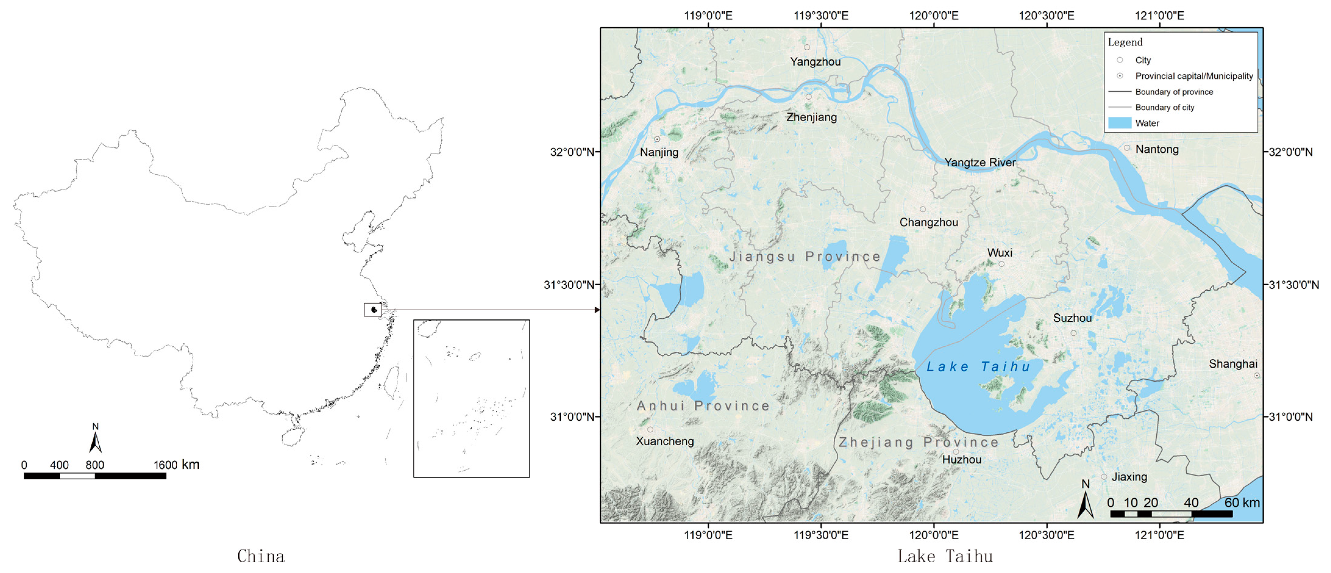
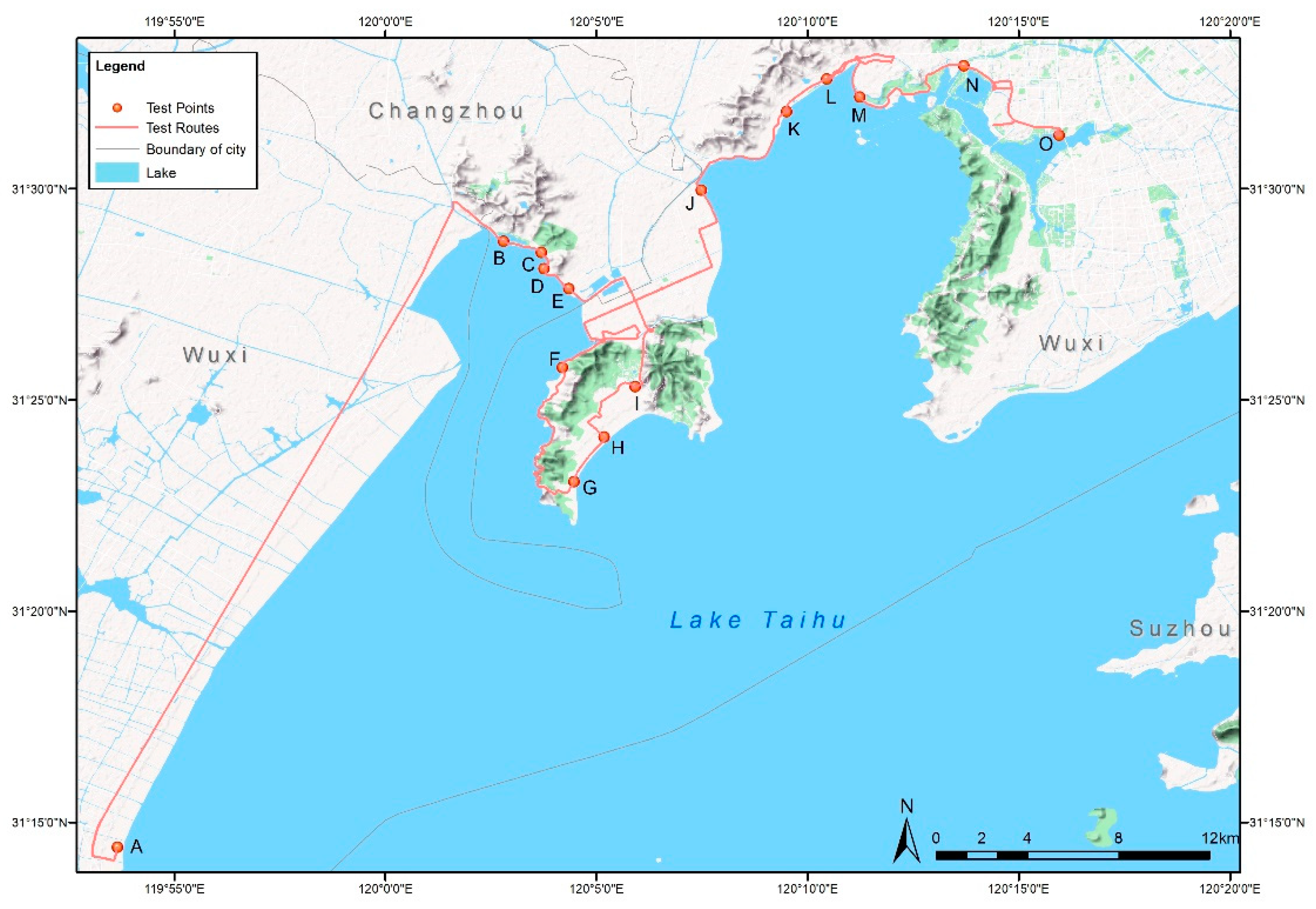
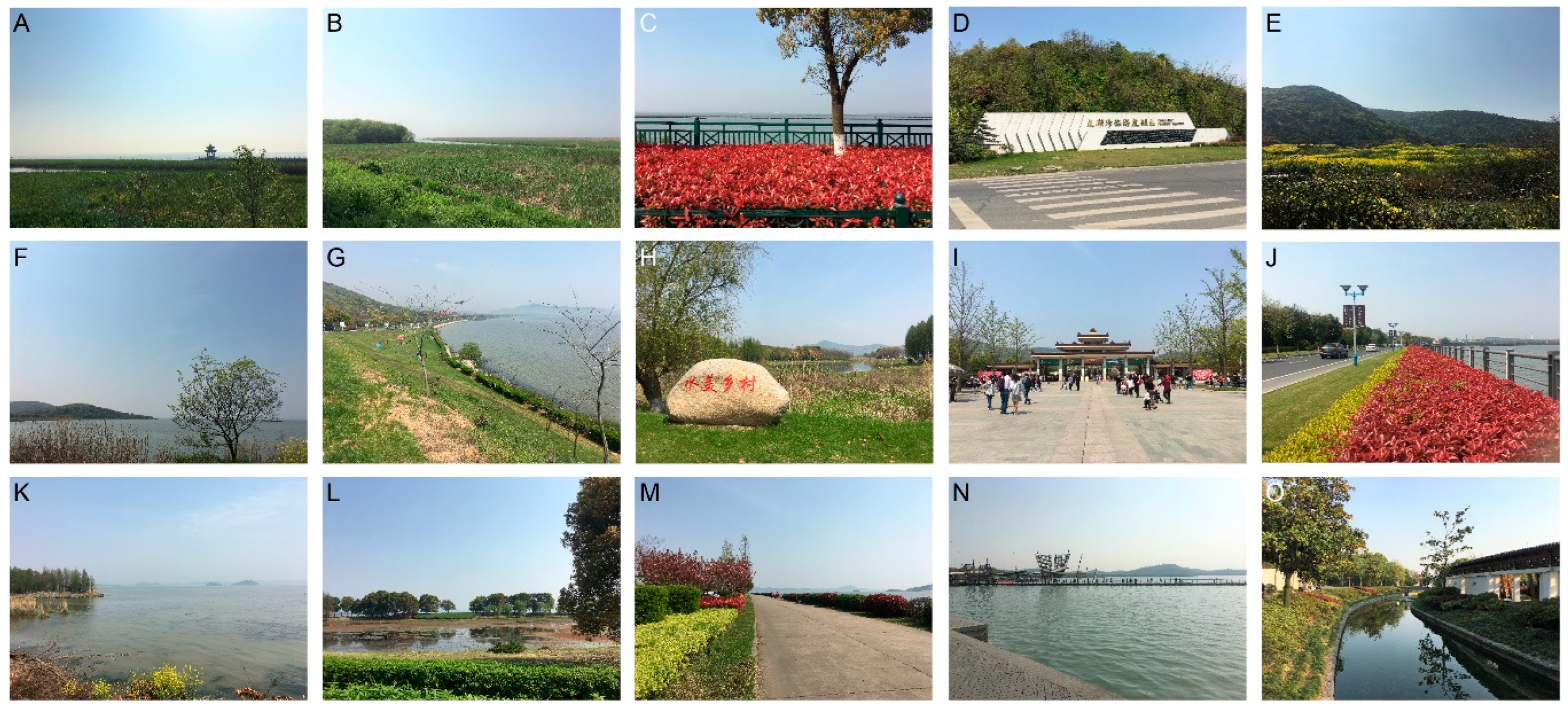
2.1. Study Area
2.2. Experimental Data Investigated
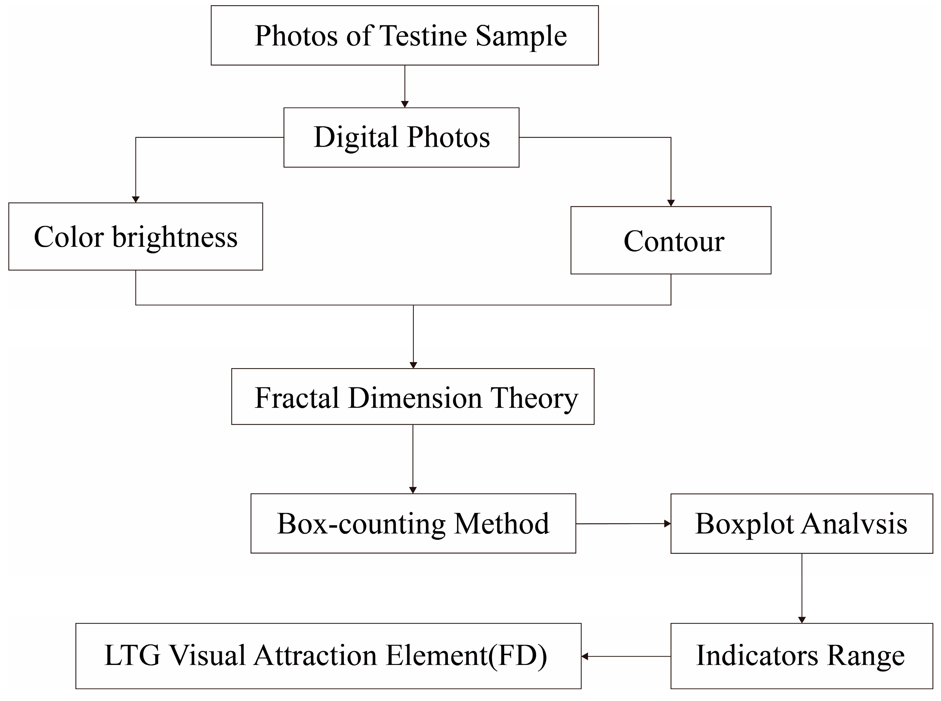
2.3. Methods
2.3.1. The Theory of Fractional Dimensionality and Its Methods
Fractal Dimension
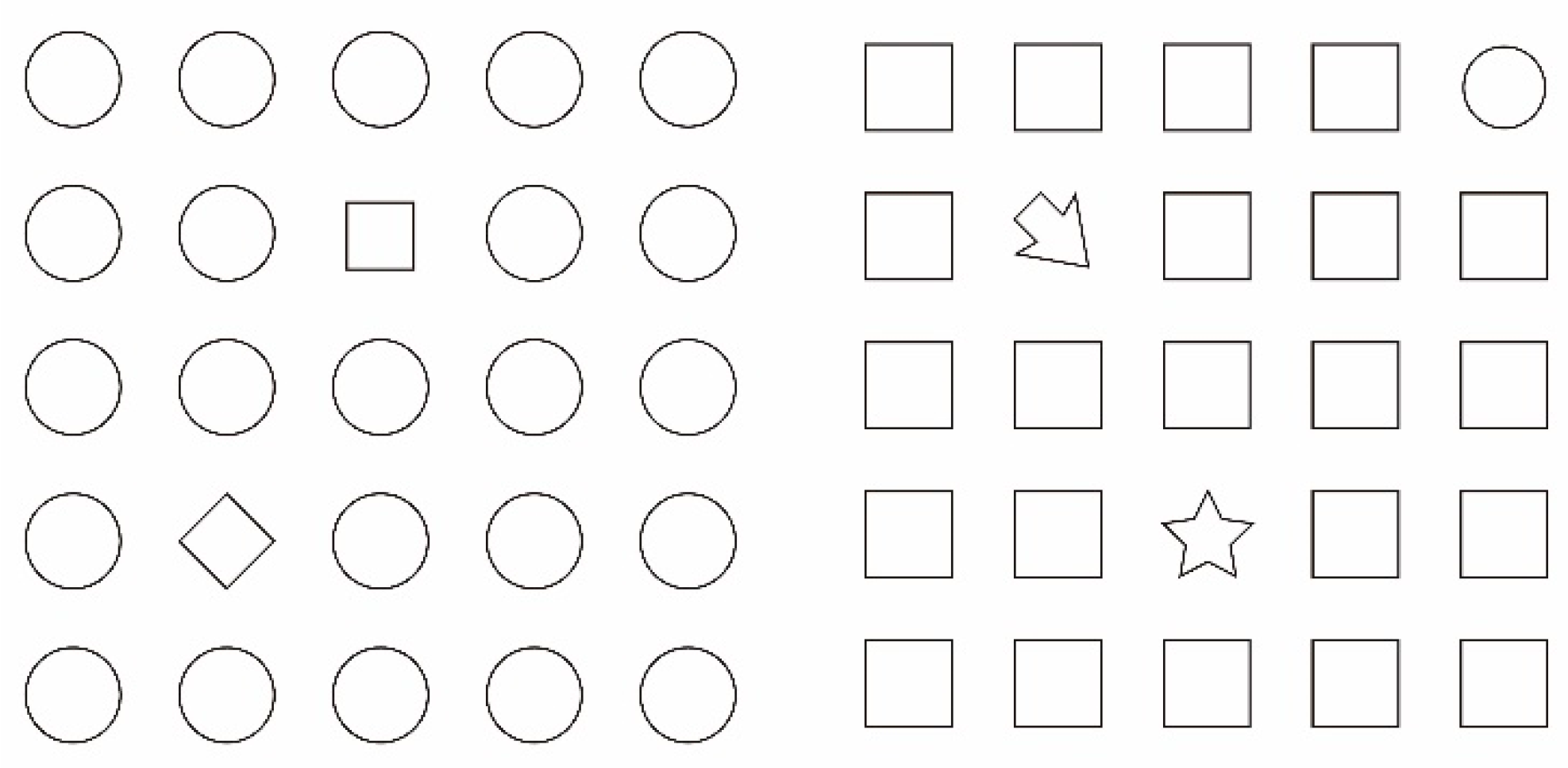
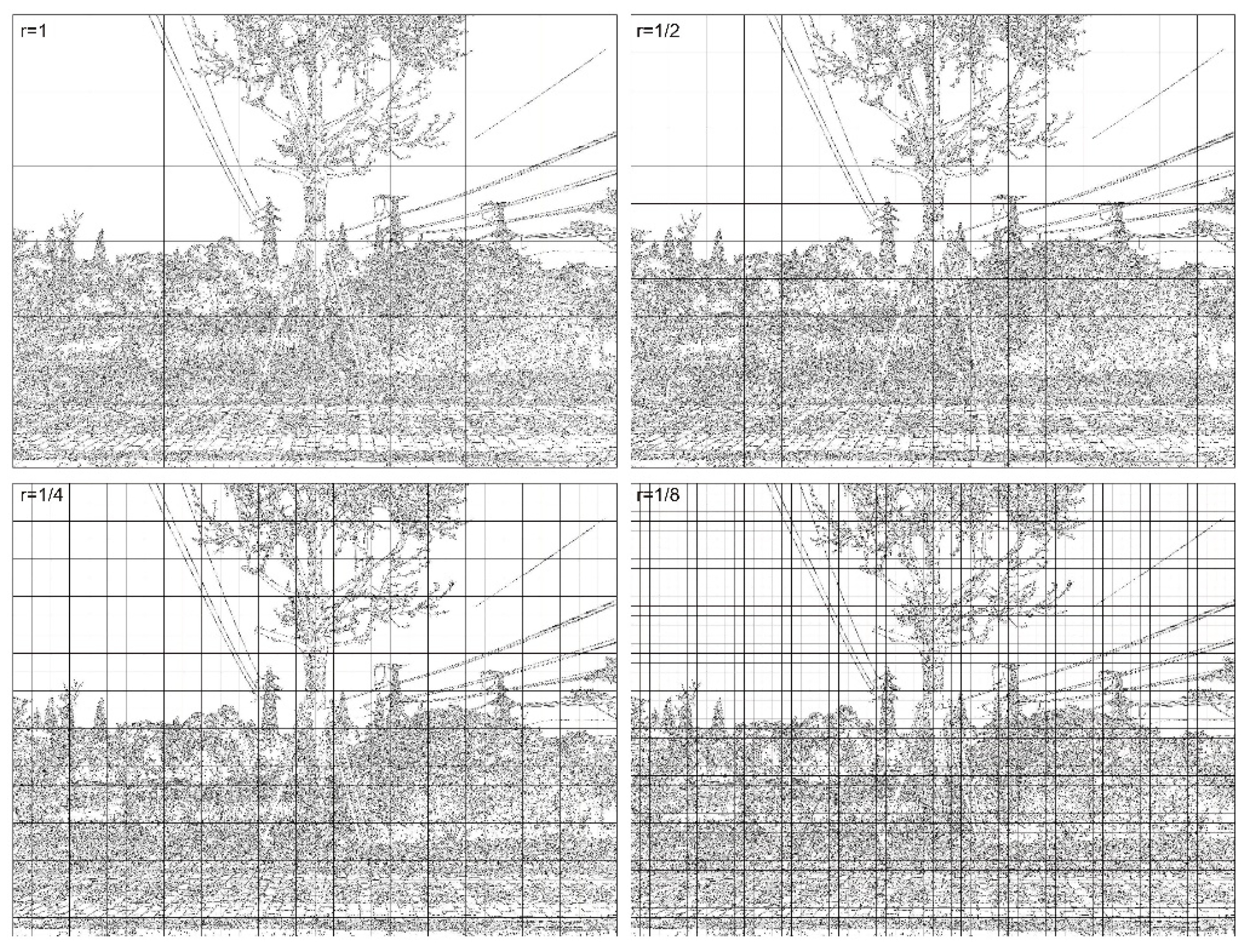
Box-Counting Fractal Dimension
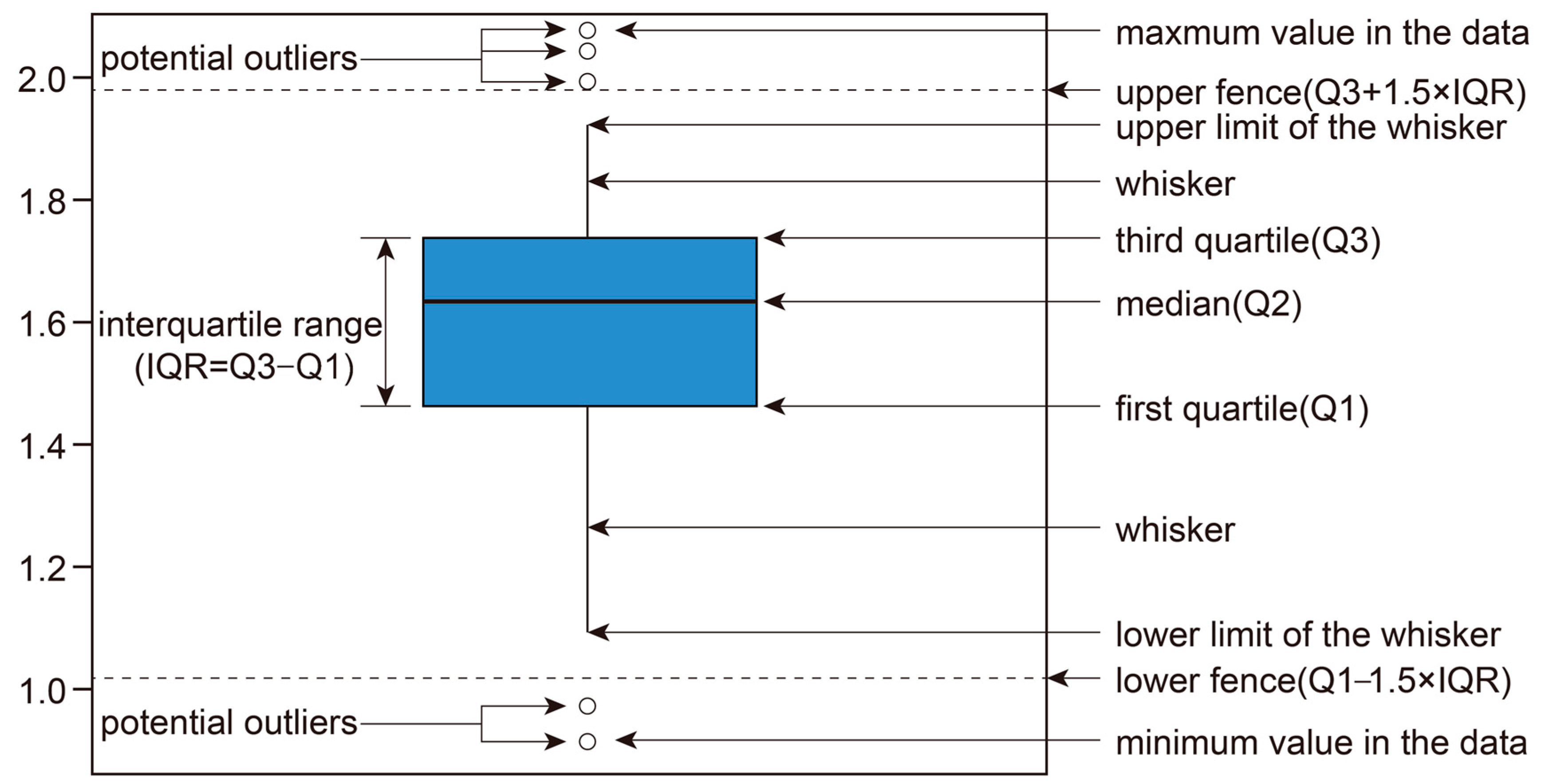
Boxplot Analysis
2.3.2. Analysis
3. Results
3.1. Overview
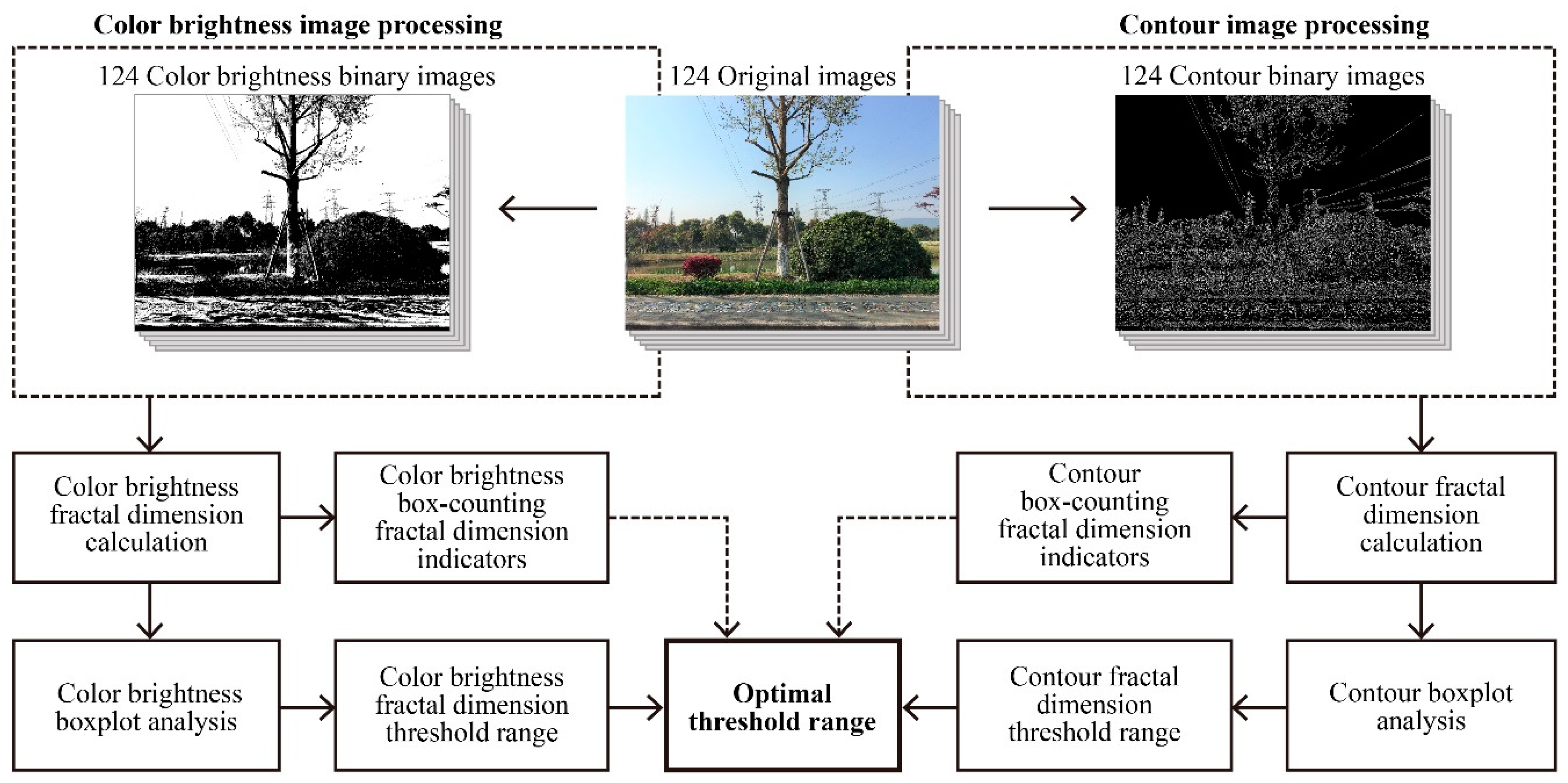
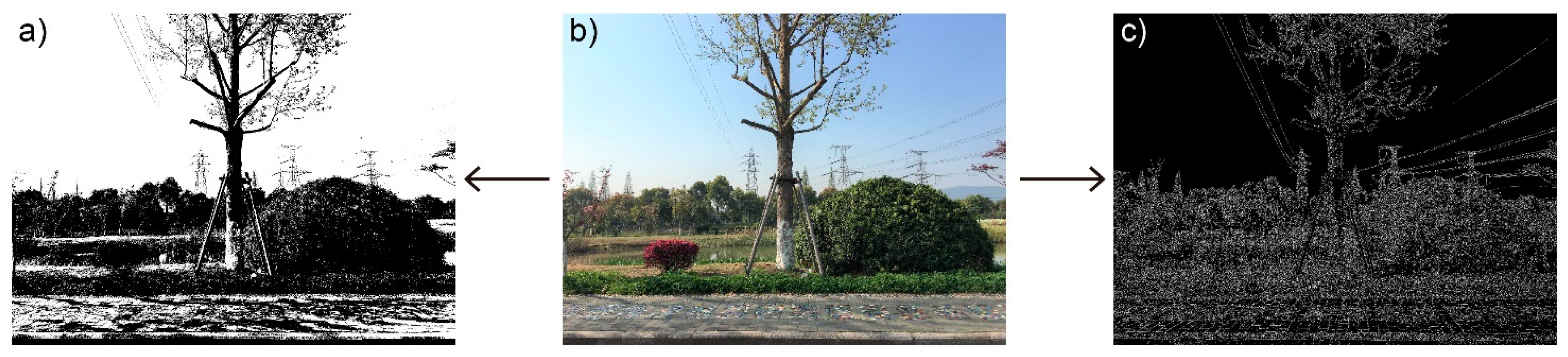
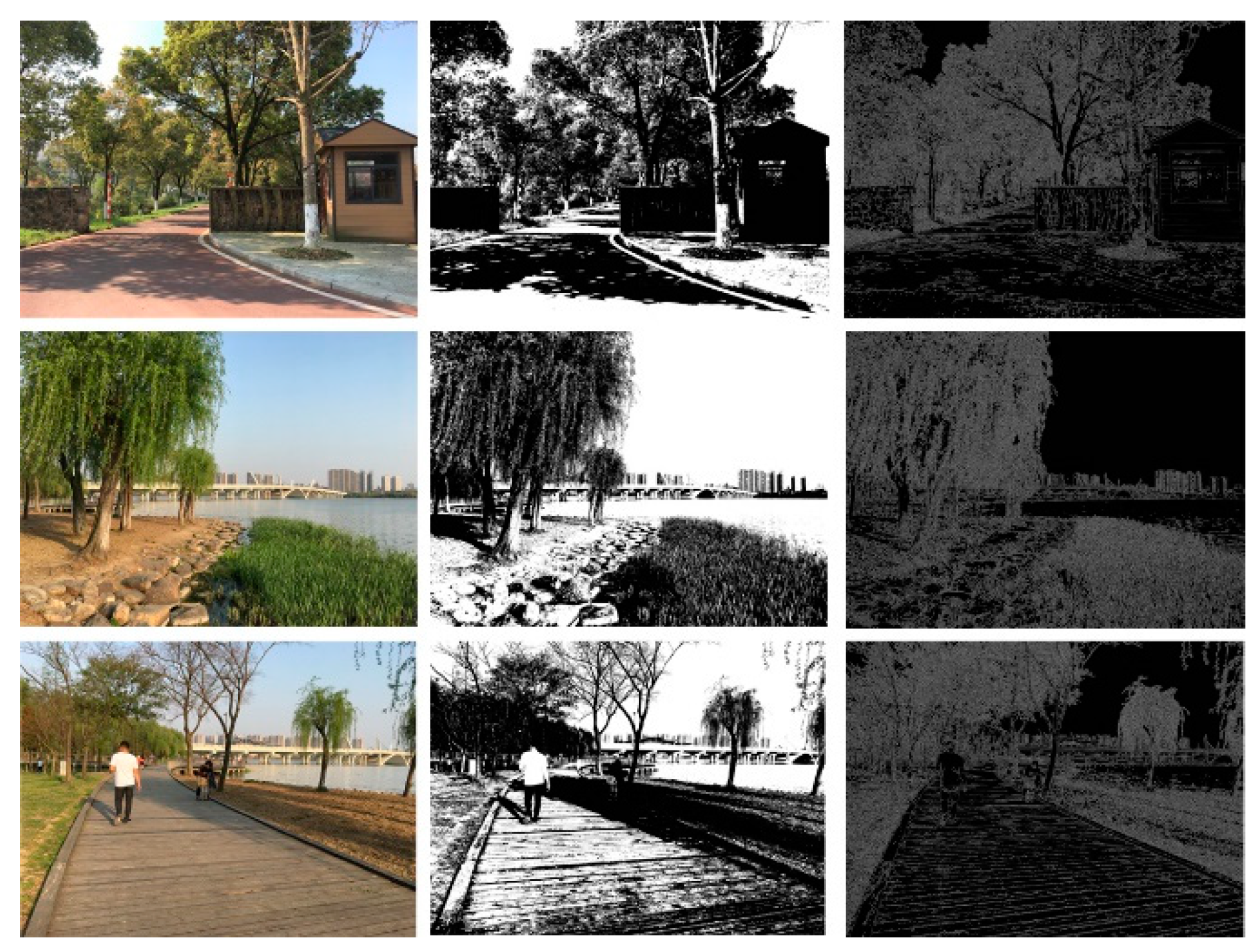
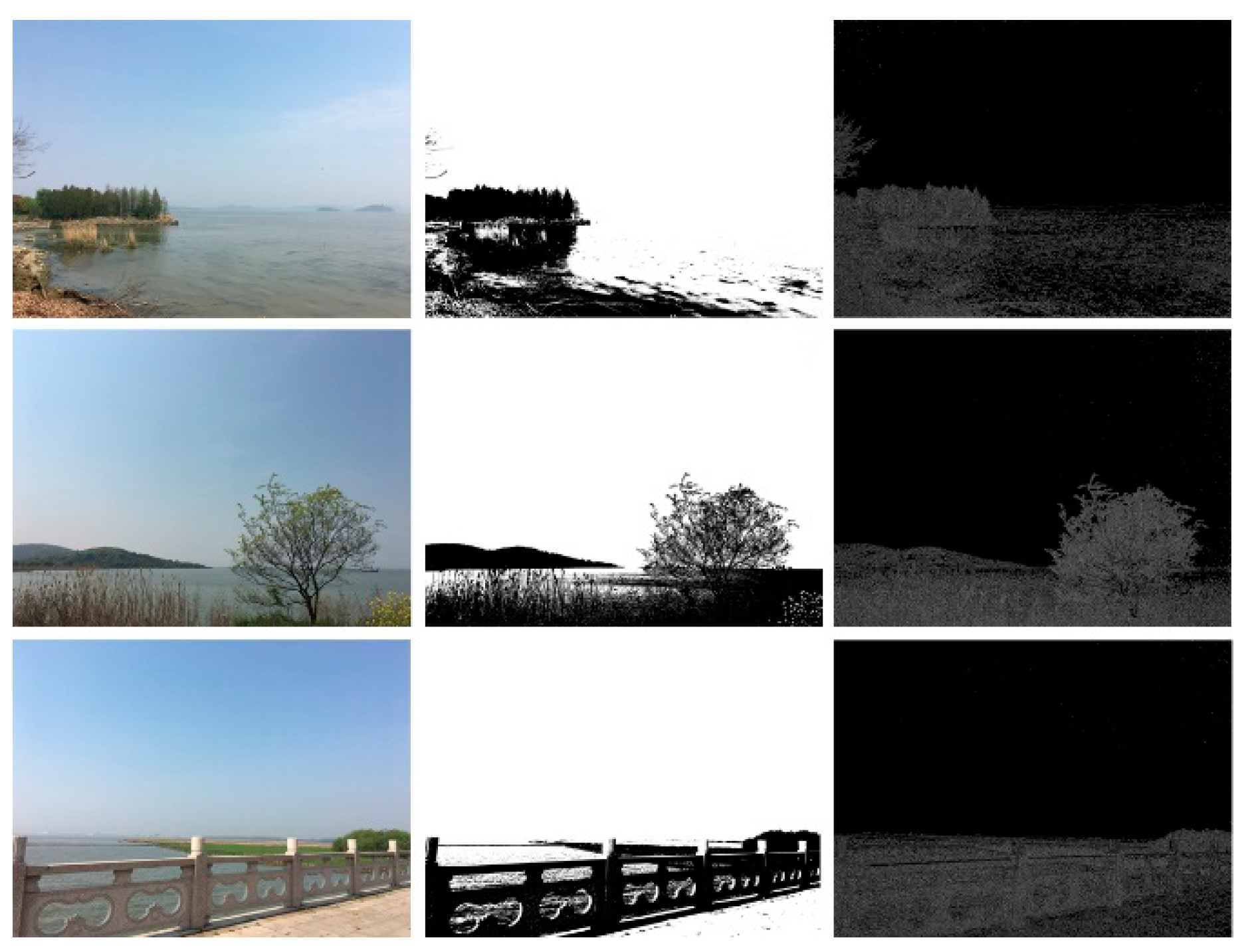
3.2. Image Processing Process and Dimensional Calculation
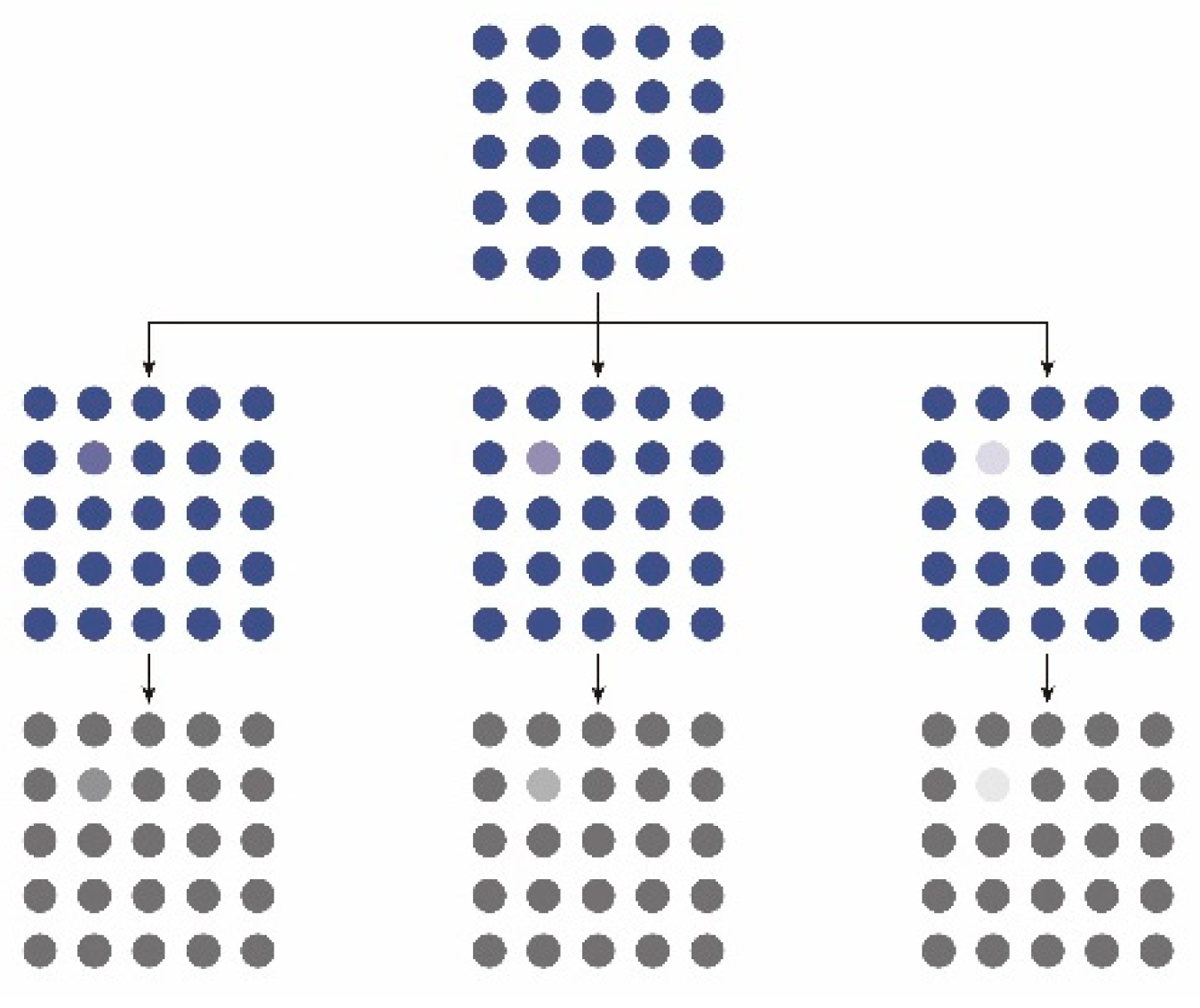
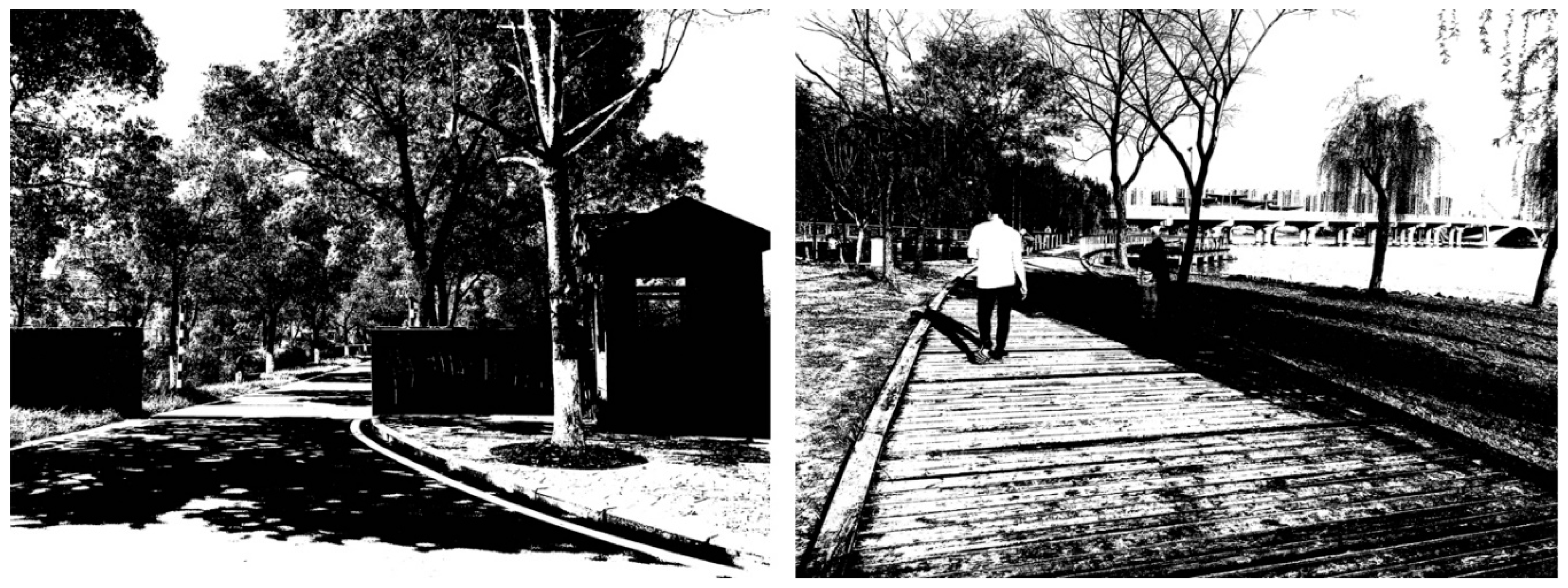
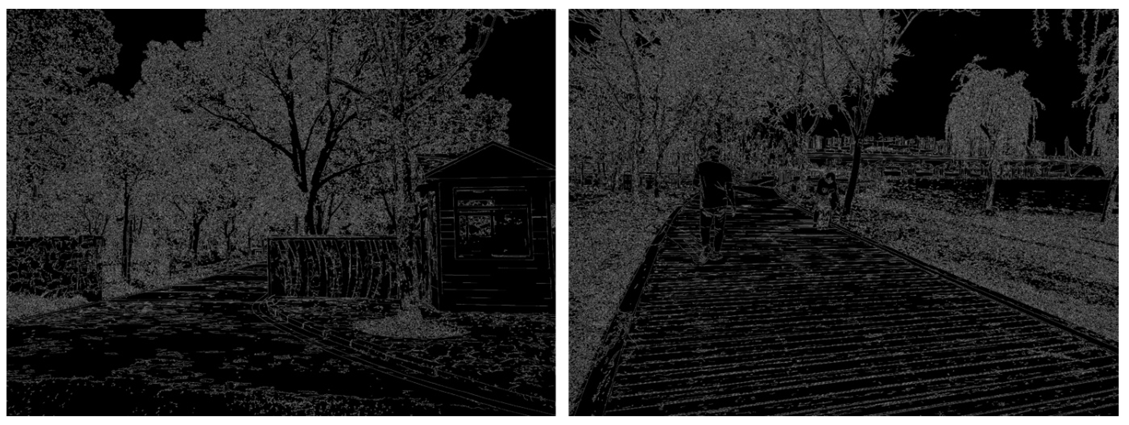
3.2.1. Image Processing Process
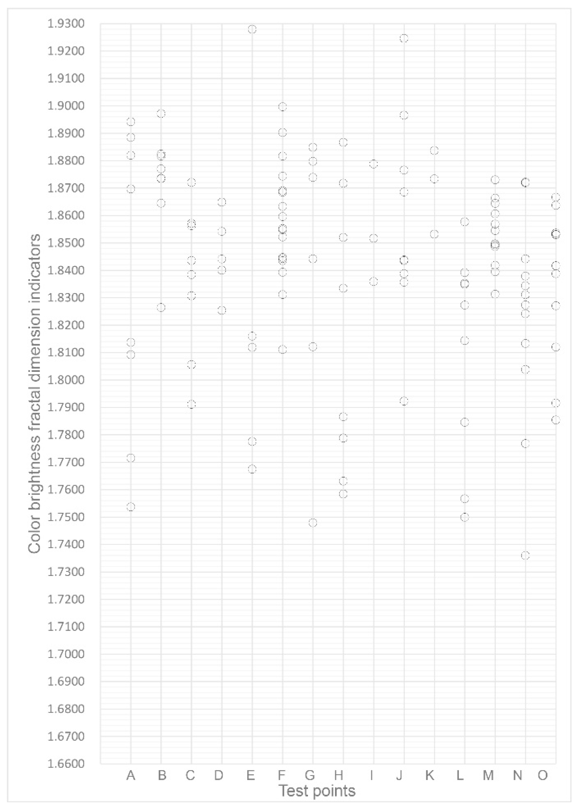
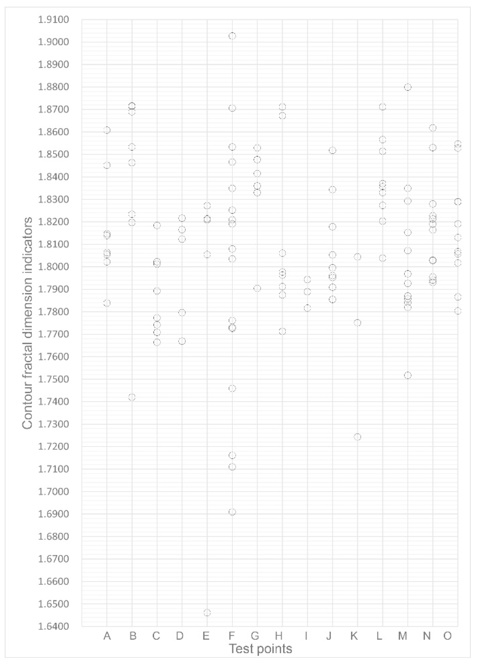
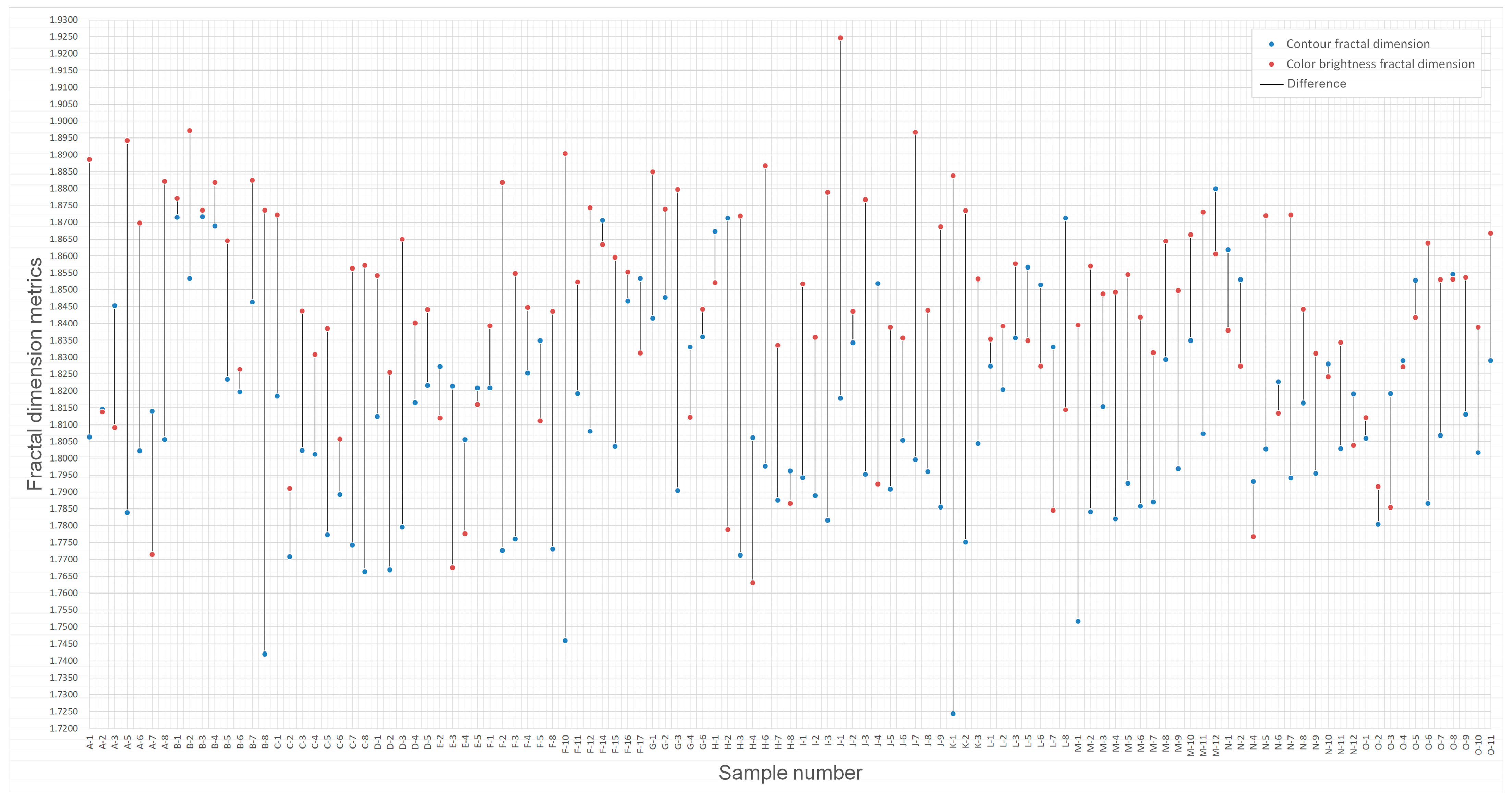
3.2.2. Box-Counting Fractal Dimension Calculation
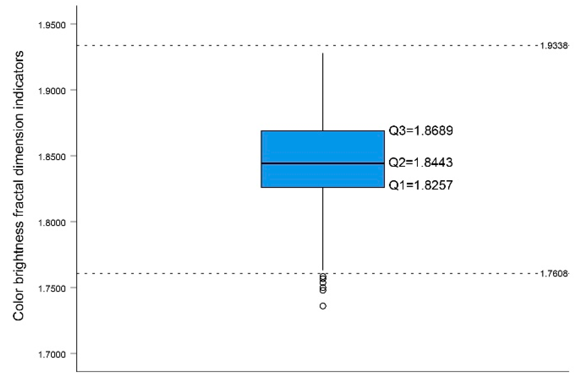
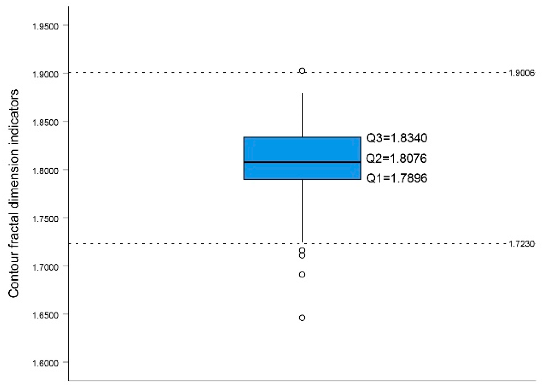
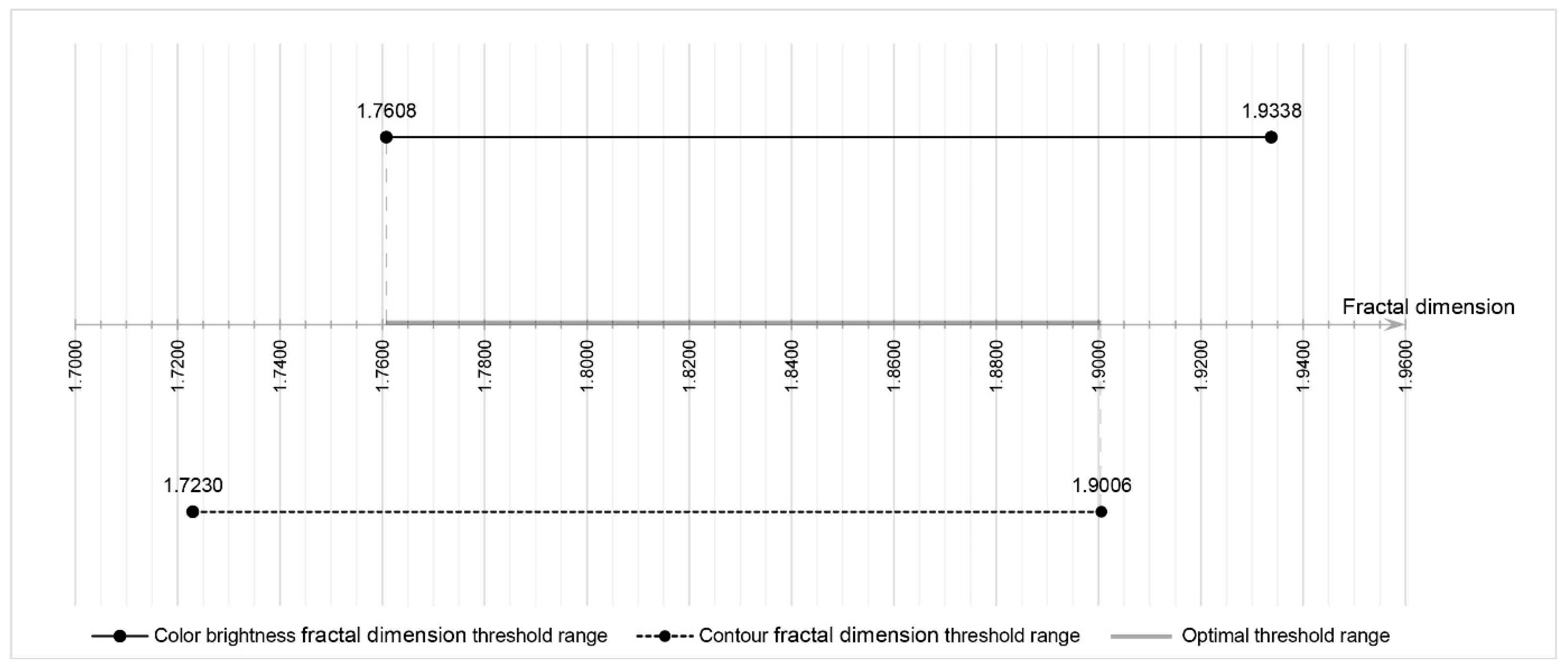
3.3. Boxplot Analysis Threshold
4. Discussion
4.1. Visual Attraction Elements of Color Brightness and Contour
4.2. Interpreting Observed Elements of Visual Attraction in Relation to the Distribution of Greenways and Water Bodies
4.3. Theoretical and Practical Implications for Regional Planning and Design
4.3.1. Theoretical Implications for Regional Planning
4.3.2. Practical Significance towards Resource Quality Enhancement
4.4. Limitations
5. Conclusions
Author Contributions
Funding
Data Availability Statement
Conflicts of Interest
References
- Little, C.E. Greenways for America; Johns Hopkins University Press: Baltimore, MD, USA, 1990. [Google Scholar]
- Furuseth, O.J.; Altman, R.E. Who’s on the greenway: Socioeconomic, demographic, and locational characteristics of greenway users. Environ. Manag. 1991, 15, 329–336. [Google Scholar] [CrossRef]
- Zhang, F.; Wu, F. Performing the ecological fix under state entrepreneurialism: A case study of Taihu New Town, China. Urban Stud. 2022, 59, 1068–1084. [Google Scholar] [CrossRef]
- Sun, S.C.; Mao, R. An introduction to lake Taihu. Lake Taihu, China: Dynamics and Environmental Change; Springer: Berlin/Heidelberg, Germany, 2008; pp. 1–67. [Google Scholar]
- Wu, Y.Y.; Wang, C.; Zhang, Z.Y.; Ge, Y. Subsistence, Environment, and Society in the Taihu Lake Area during the Neolithic Era from a Dietary Perspective. Land 2022, 11, 1229. [Google Scholar] [CrossRef]
- Li, Y.; Zheng, N. Integral Protection of Cultural Heritage of the Grand Canal of China: A Perspective of Cultural Spaces. Front. Soc. Sci. Technol. 2020, 2, 60–69. [Google Scholar]
- Thomson, S.L.; Ochoa, G.; Verel, S. The fractal geometry of fitness landscapes at the local optima level. Nat. Comput. 2022, 21, 1–17. [Google Scholar] [CrossRef]
- Li, J.; Zhong, Y.Z.; Li, Y.N.; Hu, W.; Deng, J.Y.; Pierskalla, C.; Zhang, F.A. Past Experience, Motivation, Attitude, and Satisfaction: A Comparison between Locals and Tourists for Taihu Lake International Cherry Blossom Festival. Forests 2022, 13, 1608. [Google Scholar] [CrossRef]
- Bai, Y.; Chen, Y.; Alatalo, J.M.; Yang, Z.Q.; Jiang, B. Scale effects on the relationships between land characteristics and ecosystem services- a case study in Taihu Lake Basin. China Sci. Total Environ. 2020, 716, 137083. [Google Scholar] [CrossRef]
- Xu, L.T.; Chen, S.S.; Xu, Y.; Li, G.; Su, W.Z. Impacts of Land-Use Change on Habitat Quality during 1985–2015 in the Taihu Lake Basin. Sustainability 2019, 11, 3513. [Google Scholar] [CrossRef] [Green Version]
- Su, W.Z.; Gu, C.L.; Yang, G.S.; Chen, S.; Zhen, F. Measuring the impact of urban sprawl on natural landscape pattern of the Western Taihu Lake watershed, China. Landsc. Urban Plan. 2010, 95, 61–67. [Google Scholar] [CrossRef]
- Wang, Y.N.; Li, B.; Yang, G.S. Stream water quality optimized prediction based on human activity intensity and landscape metrics with regional heterogeneity in Taihu Basin, China. Environ. Sci. Pollut. Res. 2023, 30, 4986–5004. [Google Scholar] [CrossRef]
- Bell, S. Elements of Visual Design in the Landscape, 2nd ed.; Spon Press: New York, NY, USA, 2004. [Google Scholar]
- Fan, R. Evaluation of Visual Attraction of Landscape Spaces Using Analytic Hierarchy Process. J. Chin. Urban For. 2016, 14, 74–77. [Google Scholar] [CrossRef]
- Fan, R. Visual Attraction Mechanism and Assessment of Landscape Space; Tongji University Press: Shanghai, China, 2016. [Google Scholar]
- Fan, R.; Li, W.Z.; Wu, R. Study on Spatial Visual Attraction of Landscape Space Around Lake Taihu Greenway Based on UAV Image Segmentation. Chin. Landsc. Archit. 2019, 35, 74–79. [Google Scholar]
- Skums, P.; Bunimovich, L. Graph fractal dimension and the structure of fractal networks. J. Complex Netw. 2020, 8, cnaa037. [Google Scholar] [CrossRef] [PubMed]
- Ebrahimi, M.; Bohun, S. Single image super-resolution via non-local normalized graph Laplacian regularization: A self-similarity tribute. Commun. Nonlinear Sci. Numer. Simul. 2021, 93, 105508. [Google Scholar] [CrossRef]
- Forsythe, A.; Nadal, M.; Sheehy, N.; Cela-Conde, C.J.; Sawey, M. Predicting beauty: Fractal dimension and visual complexity in art. Br. J. Psychol. 2011, 102, 49–70. [Google Scholar] [CrossRef] [Green Version]
- Chen, H.; Zheng, X. Improved Newton Iterative Algorithm for Fractal Art Graphic Design. Complexity 2020, 2020, 6623049. [Google Scholar] [CrossRef]
- Mandelbrot, B.B. The Fractal Geometry of Nature; W.H. Freeman: San Fransisco, CA, USA, 1983. [Google Scholar]
- Eke, A.; Herman, P.; Kocsis, L.; Kozak, L.R. Fractal characterization of complexity in temporal physiological signals. Physiol. Meas. 2002, 23, R1. [Google Scholar] [CrossRef] [Green Version]
- Weaver, W. Science and complexity. Am. Sci. 1948, 36, 536–544. [Google Scholar]
- Sun, W.; Kim, S.W. Visual Preference Analysis of Landscape Elements in Urban Scenic Areas of China. J. Recreat. Landsc. 2019, 13, 31–38. [Google Scholar]
- Polat, A.T.; Akay, A. Relationships between the visual preferences of urban recreation area users and various landscape design elements. Urban For. Urban Green. 2015, 14, 573–582. [Google Scholar] [CrossRef]
- Zhang, H.; Lin, S.H. Affective appraisal of residents and visual elements in the neighborhood: A case study in an established suburban community. Landsc. Urban Plan. 2011, 101, 11–21. [Google Scholar] [CrossRef]
- National Development and Reform Commission. The Overall Programme of Comprehensive Management for Water Environment of Taihu Lake Basin. 2013. Available online: https://www.ndrc.gov.cn/xxgk/zcfb/tz/201401/W020190905508283518222.pdf (accessed on 19 February 2023).
- Xu, X.; Yang, G.; Tan, Y.; Zhuang, Q.; Li, H.; Wan, R.; Su, W.; Zhang, J. Ecological risk assessment of ecosystem services in the Taihu Lake Basin of China from 1985 to 2020. Sci. Total Environ. 2016, 554, 7–16. [Google Scholar] [CrossRef] [PubMed]
- Mandelbrot, B.B. How long is the coast of Britain? Statistical self-similarity and fractional dimension. Science 1967, 156, 636–638. [Google Scholar] [CrossRef] [Green Version]
- Mandelbrot, B.B. Fractals: Form, Chance and Dimension; W.H. Freeman: San Francisco, CA, USA, 1977. [Google Scholar]
- Huang, A.S.H.; Lin, Y.J. The effect of landscape colour, complexity and preference on viewing behaviour. Landsc. Res. 2020, 45, 214–227. [Google Scholar] [CrossRef]
- Daniel Brandeis, D.; Lehmann, D. Segments of event-related potential map series reveal landscape changes with visual attention and subjective contours. Electroencephalogr. Clin. Neurophysiol. 1989, 73, 507–519. [Google Scholar] [CrossRef]
- Zhang, Z.; Qie, G.; Wang, C.; Jiang, S.; Li, X.; Li, M. Application of eye-tracking assistive technology in forest landscape evaluation. World For. Res. 2017, 30, 19–23. [Google Scholar]
- Wu, X.; Chen, S.; Zhao, R. Analysis of impact factors on forest park passenger flow based on baidu index. For. Resour. Manag. 2017, 1, 27. [Google Scholar]
- Vaughan, J.; Ostwald, M.J. Measuring the geometry of nature and architecture: Comparing the visual properties of frank Lloyd wright’s falling water and its natural setting. Open House Int. 2022, 47, 51–67. [Google Scholar] [CrossRef]
- Voss, R.F. Random fractal forgeries. Fundam. Algorithms Comput. Graph. 1985, 17, 805–835. [Google Scholar]
- Voss, R.F. Random Fractals: Characterization and measurement. Scaling Phenomena in Disordered Systems; Springer: Boston, MA, USA, 1986; Volume 27–32. [Google Scholar] [CrossRef]
- Peitgen, H.O.; Jürgens, H.; Saupe, D. Chaos and Fractals: New Frontiers of Science; Springer-Verlag: New York, NY, USA, 1992. [Google Scholar]
- Stamps, A.E. Fractals, skylines, nature and beauty. Landsc. Urban Plan. 2002, 60, 163–184. [Google Scholar] [CrossRef]
- Dasgupta, R. Determination of the fractal dimension of a shore platform profile. J. Geol. Soc. India 2013, 81, 122–128. [Google Scholar] [CrossRef]
- D’Alessandro, L.; De Pippo, T.; Donadio, C.; Mazzarella, A.; Miccadei, E. Fractal dimension in Italy: A geomorphological key to interpretation. Z. Fur Geomorphol. 2006, 50, 479–499. [Google Scholar] [CrossRef]
- Sala, N. Fractal geometry in the arts: An overview across the different cultures. Think. Patterns 2004, 177–188. [Google Scholar]
- Bourchtein, A.; Bourchtein, L.; Naoumova, N. On the visual complexity of built and natural landscapes. Fractals-Complex Geom. Patterns Scaling Nat. Soc. 2014, 22, 1450008. [Google Scholar] [CrossRef]
- Dubuc, B.; Quiniou, J.F.; Roques-Carmes, C.; Tricot, C.; Zucker, S.W. Evaluating the fractal dimension of profiles. Phys. Rev. A 1989, 39, 1500. [Google Scholar] [CrossRef]
- Schroeder, M. Fractals, Chaos, Power Laws: Minutes from an Infinite Paradise; W. H. Freeman: New York, NY, USA, 1991; pp. 41–45. [Google Scholar]
- Tukey, J.W. Exploratory Data Analysis. Reading; Addison-Wesley Publishing Company: Boston, MA, USA, 1977. [Google Scholar]
- Benjamini, Y. Opening the box of a boxplot. Am. Stat. 1988, 42, 257–262. [Google Scholar] [CrossRef]
- Frigge, M.; Hoaglin, D.C.; Iglewicz, B. Some Implementations of the Boxplot. Am. Stat. 1989, 43, 50–54. [Google Scholar] [CrossRef]
- Ferreira, J.E.V.; Miranda, R.M.; Figueiredo, A.F.; Barbosa, J.P.; Brasil, E.M. Box-and-Whisker Plots Applied to Food Chemistry. J. Chem. Educ. 2016, 93, 2026–2032. [Google Scholar] [CrossRef]
- Al-Hamdan, M.; Cruise, J.; Rickman, D.; Quattrochi, D. Effects of Spatial and Spectral Resolutions on Fractal Dimensions in Forested Landscapes. Remote Sens. 2010, 2, 611–640. [Google Scholar] [CrossRef] [Green Version]
- Juliani, A.W.; Bies, A.J.; Boydston, C.R.; Taylor, R.P.; Sereno, M.E. Navigation performance in virtual environments varies with fractal dimension of landscape. J. Environ. Psychol. 2016, 47, 155–165. [Google Scholar] [CrossRef] [Green Version]
- Liu, S. Application of big data technology in urban greenway design. Secur. Commun. Netw. 2022, 2022, 4826523. [Google Scholar] [CrossRef]
- Lu, J.; Wu, X. Research on Urban Greenway Alignment Selection Based on Multisource Data. Sustainability 2022, 14, 12382. [Google Scholar] [CrossRef]
- Gobster, P.H.; Westphal, L.M. The human dimensions of urban greenways: Planning for recreation and related experiences. Landsc. Urban Plan. 2004, 68, 147–165. [Google Scholar] [CrossRef]
- Yang, B.E.; Brown, T.J. A cross-cultural comparison of preferences for landscape styles and landscape elements. Environ. Behav. 1992, 24, 471–507. [Google Scholar] [CrossRef]
- Nordh, H.; Hartig, T.; Hagerhall, C.M.; Fry, G. Components of small urban parks that predict the possibility for restoration. Urban For. Urban Green. 2009, 8, 225–235. [Google Scholar] [CrossRef]
- Ding, M.; Zhang, Q.; Li, G.; Li, W.; Chen, F.; Wang, Y.; Li, Q.; Qu, Z.; Fu, L. Fractal dimension-based analysis of rockery contour morphological characteristics for Chinese classical gardens south of the Yangtze River. J. Asian Archit. Build. Eng. 2023, 1–16. [Google Scholar] [CrossRef]


| Type | Elements |
|---|---|
| landscape visual elements | point, line, plane, solid volume, and open volume |
| landscape visual attraction elements | spatial scale and distance, solid, boundary, color, line, shape, transitory natural phenomenon, vegetation, texture, waterbody, dynamic scene, sunlight |
| Test Points | Latitude and Longitude Coordinates | City | Sample Size | Color Brightness Fractal Dimension Interval | Contour Fractal Dimension Interval |
|---|---|---|---|---|---|
| A | (31°14′24″ N, 119°53′38″ E) | Wuxi | 8 | (1.7537, 1.8942) | (1.7839, 1.8608) |
| B | (31°28′45″ N, 120°02′47″ E) | Changzhou | 8 | (1.8264, 1.8972) | (1.7420, 1.8716) |
| C | (31°28′29″ N, 120°03′41″ E) | Changzhou | 8 | (1.7911, 1.8721) | (1.7664, 1.8184) |
| D | (31°28′06″ N, 120°03′45″ E) | Changzhou | 5 | (1.8254, 1.8649) | (1.7669, 1.8216) |
| E | (31°27′37″ N, 120°04′20″ E) | Changzhou | 5 | (1.7675, 1.9279) | (1.6461, 1.8272) |
| F | (31°25′45″ N, 120°04′11″ E) | Wuxi | 17 | (1.8111, 1.8997) | (1.6909, 1.9027) |
| G | (31°23′03″ N, 120°04′27″ E) | Wuxi | 6 | (1.7479, 1.8849) | (1.7904, 1.8529) |
| H | (31°24′07″ N, 120°05′10″ E) | Wuxi | 8 | (1.7584, 1.8867) | (1.7713, 1.8712) |
| I | (31°25′18″ N, 120°05′54″ E) | Wuxi | 3 | (1.8359, 1.8788) | (1.7816, 1.7943) |
| J | (31°29′57″ N, 120°07′28″ E) | Wuxi | 9 | (1.7923, 1.9246) | (1.7855, 1.8518) |
| K | (31°31′49”N, 120°09′30″ E) | Wuxi | 3 | (1.8532, 1.8837) | (1.7243, 1.8044) |
| L | (31°32′35”N, 120°10′27″ E) | Wuxi | 9 | (1.7499, 1.8577) | (1.8039, 1.8712) |
| M | (31°32′09”N, 120°11′13″ E) | Wuxi | 12 | (1.8313, 1.8730) | (1.7517, 1.8799) |
| N | (31°32′54”N, 120°13′41″ E) | Wuxi | 12 | (1.7360, 1.8722) | (1.7931, 1.8618) |
| O | (31°31′15”N, 120°15′57″ E) | Wuxi | 11 | (1.7854, 1.8667) | (1.7804, 1.8546) |
| The Boxplot Calculation | The Boxplot Results | ||||
|---|---|---|---|---|---|
| Threshold Range | Outliers | Sample Number of Outliers | |||
| Color brightness boxplot | |||||
| Q1 | 1.8257 | (1.7608, 1.9337) | 1.7360 1.7479 1.7499 1.7537 1.7567 1.7584 | N-3 G-5 L-9 A-4 L-4 H-5 | |
| Q2 | 1.8443 | ||||
| Q3 | 1.8689 | ||||
| IQR | 0.0432 | ||||
| Contour boxplot | |||||
| Q1 | 1.7896 | (1.7230, 1.9006) | 1.6461 1.6909 1.7110 1.7161 1.9027 | E-1 F-6 F-7 F-9 F-13 | |
| Q2 | 1.8076 | ||||
| Q3 | 1.8340 | ||||
| IQR | 0.0444 | ||||
| Sample Number | Fractal Dimension Metrics | ||
|---|---|---|---|
| Color Brightness Fractal Dimension | Contour Fractal Dimension | Absolute Value of Difference | |
| Three samples with the smallest difference | |||
| A-2 | 1.8137 | 1.8146 | 0.0009 |
| O-8 | 1.8531 | 1.8546 | 0.0015 |
| O-4 | 1.8271 | 1.8289 | 0.0018 |
| Three samples with the largest difference | |||
| K-1 | 1.8837 | 1.7243 | 0.1594 |
| F-10 | 1.8903 | 1.7459 | 0.1444 |
| B-8 | 1.8735 | 1.7420 | 0.1315 |
Disclaimer/Publisher’s Note: The statements, opinions and data contained in all publications are solely those of the individual author(s) and contributor(s) and not of MDPI and/or the editor(s). MDPI and/or the editor(s) disclaim responsibility for any injury to people or property resulting from any ideas, methods, instructions or products referred to in the content. |
© 2023 by the authors. Licensee MDPI, Basel, Switzerland. This article is an open access article distributed under the terms and conditions of the Creative Commons Attribution (CC BY) license (https://creativecommons.org/licenses/by/4.0/).
Share and Cite
Fan, R.; Yocom, K.P.; Guo, Y. Utilizing Fractal Dimensions as Indicators to Detect Elements of Visual Attraction: A Case Study of the Greenway along Lake Taihu, China. Land 2023, 12, 883. https://doi.org/10.3390/land12040883
Fan R, Yocom KP, Guo Y. Utilizing Fractal Dimensions as Indicators to Detect Elements of Visual Attraction: A Case Study of the Greenway along Lake Taihu, China. Land. 2023; 12(4):883. https://doi.org/10.3390/land12040883
Chicago/Turabian StyleFan, Rong, Ken P. Yocom, and Yeyuan Guo. 2023. "Utilizing Fractal Dimensions as Indicators to Detect Elements of Visual Attraction: A Case Study of the Greenway along Lake Taihu, China" Land 12, no. 4: 883. https://doi.org/10.3390/land12040883