Article

Debris Flow Gully Classification and Susceptibility Assessment Model Construction

1
Key Research Institute of Yellow River Civilization and Sustainable Development and Collaborative Innovation Center on Yellow River Civilization Jointly Built by Henan Province and Ministry of Education, Henan University, Kaifeng 475001, China
2
Department of Earth Sciences, The University of Haripur, Haripur 22620, Pakistan
3
School of Cultural Industry & Tourism Management, Henan University, Kaifeng 475001, China
*
Author to whom correspondence should be addressed.
Land 2023, 12(3), 571; https://doi.org/10.3390/land12030571
Submission received: 22 January 2023 / Revised: 19 February 2023 / Accepted: 24 February 2023 / Published: 26 February 2023
(This article belongs to the Special Issue New Perspectives for the Monitoring and Early Detection of Geohazards)

Abstract

:
The location of debris flow occurring in a gully determines the observable differences in its formation, evolution and effects. In this piece of research, we propose a new method for debris flow gully classification based on the locations of the debris flows occurring in the gullies. It is termed the three-section method (TSM). It includes eight different types of gullies with different digital identifications (IDs) and susceptibility degrees (SDs). By taking the Jiangjia Gully (JJG), in Yunnan, China, as a case study site, the main gully and the sub-gullies at different levels were identified using a hydrological analysis method. Then, the gullies were divided into different types using the new classification TSM. The results show that there are seven different types of debris flow gullies in the JJG. The number of different types varied greatly in gullies at different levels. In particular, the topological diagram of debris flow gullies was drawn after simplifying the shape of the gullies, and it was a good way to understand the characteristics of debris flow gullies. Finally, the relationships were explored between the hypsometric integrals (HIs), surface exposures (SEs) and susceptibility degrees (SDs), and a new calculation model construction method for determining the degree of debris flow susceptibility was proposed. This model, using the above method, can not only be used to calculate the SDs of debris flows in the gullies, but can also be instrumental in pointing out the approximate locations of the debris flow commonly and easily occurring in the gullies. We hope that our research can provide a new concept for the assessment of debris flow susceptibility.

1. Introduction

A gully is a landform generated by the rapid erosion of water on hillsides [1]. Erosion caused by surface runoff can often provide a rich material source for the formation of debris flows, and can accelerate the formation of gullies [2,3]. Normally, a gully in which debris flows have occurred can be described as a debris flow gully [4,5]. Researchers often use the alluvial fans of debris flows at the outlet of the gullies as the defining marks in order to evaluate whether they are debris flow gullies [6,7]. We need to realize that, for a gully in which debris flows occur, the locations of the debris flows in the gully may differ and consequently the characteristics of the gully may also differ [8]. This has been recognized by some researchers, but little in-depth research has been carried out. Generally, debris flows may accumulate at the mouth of the gullies, forming the accumulation area. However, if the terrain begins to become flat at the halfway point of the movement, debris flows can also begin to accumulate. After the sediment decreases due to the continuous movement of the fluid, the confluence from the surrounding hillsides continues to increase; therefore, the proportion of sediment and water changes, and this may evolve into high sediment-concentrated floods and form a mountain hazard chain. For the above debris flow gullies, due to the different locations of the deposition, the impact range of debris flows may be different, and may affect just the upstream, the middle or the downstream of the watershed. When Zhong et al. [9] conducted research on debris flows in Northeast China, they mentioned that when the forest coverage rate in the Laomao mountain area, in southern Liaoning, reached more than 60%, although debris flows occurred, they were small in scale and generally stopped in the branch gullies. This again shows that not all debris flow gullies can form typical debris flow gullies with gully mouth alluvial fans.
Nowadays, the study of debris flow gullies can be found in many research fields. Nistor and Church [10] researched the suspended sediment transport regime in a debris flow gully on Vancouver Island, British Columbia. Zhu [11] selected 11 factors as background parameters in order to study the judgement of debris flow gullies. Tang et al. [12] analyzed rainfall-triggered debris flows following the Wenchuan earthquake, and used the Xishanpo debris flow gully to present a case study. Debris flow gullies are often regarded as the units of debris flow disaster research, and they often appear in the assessment work of catchment unit regarding debris flow susceptibility, hazard and risk. In fact, the development and movement of debris flows are restricted by many factors such as precipitation, slope gradient, aspect, relative relief, vegetation and so on [13,14,15,16,17,18]. In a watershed, the above factors are complex; this also determines the fact that there is randomness in the whole debris flow-developing process from formation to accumulation, which may or may not affect different sections of the gullies. Tie and Tang [19] used an analytic hierarchy process (AHP) to analyze the relevant factors that affect the hazard degree of debris flow gullies, constructed a hierarchical index system, and selected two debris flow gullies in Houshan, Dongchuan City, Kunming as examples, in order to evaluate the hazard degree of debris flow hazards. Liu et al. [20] studied the quantitative determination method that ascertains the risk degree of gully-type debris flows in China, and determined and tested the risk degree of debris flow gullies in the Xiaojiang River basin. Jiang et al. [21] divided the Dadu River basin into a total of 1780 catchments using GIS spatial analysis tools with the DEM (30 m resolution), and identified a total of 281 catchments in the study area as being prone to debris flows; this was in order to use them to train the hybrid machine learning models that were created to assess the susceptibility of debris flows. On the other hand, we found that compared to using more factors to evaluate the susceptibility and hazard of debris flow gullies, fewer and more critical factors could also be used to achieve the relevant assessment research. Cui et al. [22] used a Hypsometric Integral (HI), representing the watershed geomorphologic characteristics, short-duration heavy rainfall data, representing rainfall-induced conditions, and the burn severity, representing the material source conditions in order to finish the hazard assessment of post-fire debris flows.
In our research, we try to take debris flow gullies as the research object. Firstly, a new classification method was constructed in order to distinguish debris flow gullies according to the different locations of debris flows occurring in gullies, and discussed the differences in their characteristics. Then, we defined the different susceptibility levels of several types of debris flow gully, and we also used their susceptibility degree (SD) for the digital identification (ID) of the different types of debris flow gully. Lastly, we selected the key factors, which were the Hypsometric Integral (HI) and Surface Exposure (SE), and we proposed a new calculation model construction method for determining the debris flow susceptibility degree (SD). We hope that the model constructed using our method can not only assess the susceptibility of debris flow gullies, but also distinguish the different types of debris flow gully according to the approximate speculation of the calculation results.

2. Study Area and Materials

2.1. Study Area

The Jiangjia Gully (JJG), located in the northeast of Yunnan Province, China (Figure 1a,b), is a tributary of the Xiaojiang River (Figure 1c). Affected by the subtropical monsoon, the rainfall here is mainly concentrated from May to October [23]. The JJG is a huge, frequently affected and serious rainstorm debris flow gully with a trunk channel length of 13.9 km and a total area of 48.6 km2 [24]. The JJG extends along seismic faults, and frequent earthquakes cause serious rock fragmentation. The outcrops of the rocks are mainly pre-Cambrian epimetamorphic rocks, including phyllite, slate, and shale, which are easily weathered. Quaternary diluvium and colluvium cover 80% of the JJG, providing abundant material supplies to debris flows [25]. The watershed of the JJG is characterized by weak lithology, abundant vertical and horizontal local faults, steep terrain, sparse vegetation, complex surface morphology, and very frequent landslides and collapses [26]. Known as the “Natural Museum of debris flows” in the Jinsha River system, the JJG could provide good conditions for debris flow observation, experimental research, and research on disaster prevention and reduction. In recent decades, much research on debris flow disasters has been carried out in the JJG [24,27,28,29].

2.2. Materials

DEM data and remote sensing image data are important resources for our research. Among them, DEM data come from the Advanced Land Observing Satellite (ALOS). ALOS is Japan’s Earth observation satellite, and has three sensors. The Panchromatic Remote-sensing Instrument for Stereo Mapping (PRISM) [30] of ALOS is mainly used for digital elevation mapping; the Advanced Visible and Near Infrared Radiometer type 2 (AVNIR-2) [31] can be used for accurate land observation; and the Phased-Array Synthetic-Aperture Radar (PALSAR) [32] is used for all-weather and all-time observation. PALSAR is not affected by clouds, weather and day and night, and can observe the earth all day. With a high resolution, it can obtain a wider ground view than ordinary SAR. At the same time, PALSAR can be used to generate digital elevation model (DEM) data and monitor specific areas. Now, the 12.5 m resolution ALOS PALSAR DEM data can be downloaded from NASA’s EOSDIS website [33]. During the research of this study, we downloaded the DEM data of the JJG (Figure 2a). As shown in Figure 2a, the JJG is higher in the east, with an altitude of 3228 m, and lower in the west (1036 m). The eastern area of the whole JJG watershed is wider than the western area. The watershed looks like a lying gourd-like ladle, with the mountainous area in the east of the watershed being the main catchment area.
The high-resolution remote sensing image acquired by the satellite on 23 January 2019 (Figure 2b) was downloaded from Google Earth, which is a computer program that can render a representation of Earth with the support of massive satellite images [34,35]. As an important data source, the high-resolution remote sensing image can be used to interpret the debris flows, using remote sensing images of other time periods on Google Earth for comparison and reference [36,37]. When interpreting, we also mainly interpreted the long-term stable debris flow disaster traces, so as to use them as the basic data for finding laws.
In addition, Landsat 8 data were downloaded. Landsat 8 is the eighth satellite of the Landsat program. It was launched on 11 February 2013 as an Earth observation satellite with two sensors, the Operational Land Imager (OLI) and the Thermal InfraRed Sensor (TIRS) [38]. The OLI consists of 8 bands with a spatial resolution of 30 m, and a 15 m panchromatic band, while the TIRS can provide 100 m thermal infrared images. In this study, two Landsat 8 images, taken in 2019 (Table 1), were downloaded and used to study the vegetation coverage of the JJG.

3. Methods

3.1. Susceptibility Assessment Based on the Formation Process of Debris Flows

The formation of debris flow must meet the following three important conditions [22]: (1) The existence of a large amount of loose solid materials (source) that are stored in a watershed; (2) an area with high mountains, steep slopes, and large longitudinal slopes with trenches (topographic conditions); and (3) the presence of enough water sources and catchment power areas (water source conditions). It can be seen that the rainfall factor, topographic condition factor, and material source condition factor are the key disaster-causing factors for the formation of debris flows. Nowadays, the assessment methods for determining debris flow susceptibility and hazard are relatively similar; these include logistic regression modeling [40], the Bayesian network [41], the support vector machine [41], artificial neural networks [42], etc., and the differences between them are more reflected in the selection of factors. Considering that rainfall is considered to be the triggering condition of debris flows, the hazard assessment of debris flows can be carried out together with terrain condition factors and material source condition factors; meanwhile, without considering rainfall, the terrain condition factors and material source condition factors could be used to evaluate the susceptibility of debris flow disasters [22,25] (Figure 3).

3.2. Extraction of Gully Lines and Mapping of Debris Flow Occurrences

A watershed, where precipitation collects and drains off into a common outlet, is a hydrological unit commonly used in natural resource management and planning [43]. Now, most GIS software can be used to extract watershed data, such as ArcGIS, QGIS, SAGA and so on [44,45,46]. These tools can determine the contributing area above a set of cells. We drew upon lessons regarding the relevant methods of watershed extraction for the extraction of the gully line and watershed. The whole process involves the following steps (Figure 3):
(1)
Generation of the sink filling raster image. A sink is a cell that is surrounded by higher value grids in a raster [47]. “Fill” is usually the first step of hydrological analysis. It can help to remove small imperfections in the data by changing the pixel value of a sink to the lowest pixel value around it [48] (Figure 4a).
(2)
Calculation of the flow direction raster image. DEM grids after sink filling can be used to obtain the flow direction raster from each cell to its downslope neighbor using the “Flow Direction” tool in ArcGIS. Now, the Flow Direction tool of ArcGIS supports three flow-modeling algorithms, including D8, Multi Flow Direction (MFD) and D-Infinity (DINF). The D8 method was used in this study to determine the flow direction by obtaining the direction that points to the steepest down-sloping neighbor of the surrounding 8 pixels [49,50] (Figure 4b).
(3)
Construction of the flow accumulation raster image. After obtaining the flow direction raster, the raster of flow accumulation, which lists the number of pixels flowing across it for each pixel, can be created using the “Flow Direction” tool in ArcGIS, taking the flow direction raster as the input raster [51] (Figure 4b).
(4)
Generation of the river network and the gully line raster image. In order to obtain the grid river network, the conditional function in ArcGIS can be used to set a threshold for the flow accumulation grids (Figure 4c). Xiong et al. [52] used 0.25 km2 as a threshold to identify the small watersheds of the debris flow gullies. Using this threshold as a reference, the gully lines can be obtained. Referring to the method of dividing the main stream and tributary stream [53,54], the distinction between the main gully and the sub-gully can be achieved.
(5)
Drawing of the pour points. Pour points at the outlet of each watershed need to be drawn (Figure 4c).
(6)
Extraction of the watersheds. Taking the flow direction raster and pour point data as input data, the ArcGIS “watershed” tool can help to obtain the contributing areas above the different pour points. The boundary of the contributing areas is determined as the range of watersheds (Figure 4c).
Debris flow identification, based on high-resolution remote sensing images, has been widely used [36]. Because they are rapid and are accompanied by the strong movement of debris materials along the flow path, there is much evidence that can be used to identify the occurring of debris flows, such as the traces of channel stream flow, sharp bank erosion, fallen tree trunks, and uneven debris deposits. For example, mud marks on both sides of streamways and the depositional features of sediment can be used to determine whether debris flows occur or not [22]. Moreover, they are usually associated with other landslide types, such as rockfalls and slope failures, providing a solid source around them [55]. In this study, landslide scars, vegetation changes, channel features and other factors are comprehensively considered in order to ensure the accuracy of interpretation [56].

3.3. New Classifications of the Debris Flow Gullies Using the Three-Section Method (TSM) and Definition of Susceptibility Degrees (SDs)

In general, the conditions of debris flows can change from the head to the tail of a gully. Some gully sections show the presence of debris flows, while others do not. For their characterization, we have divided a gully into three equidistant sections: “Upper Section, U-S”, “Middle Section, M-S” and “Down Section, D-S” (Figure 5a). Based on the observation and interpretation of the high-resolution remotely sensed image, the conditions of debris flows in the different sections of a gully can be evaluated. The location of a debris flow in a particular section of a gully allows the distinction of different types gullies so to tag them with identifiers. We have distinguished 8 different combinations of conditions in different sections of a gully. We termed the procedure the “three-section method (TSM)” of debris flow gully classification.
With an increase in the material carried along by the debris flows and the transformation of potential energy to kinetic energy, the possibility of debris flows occurring and destruction also increases [57]. Therefore, different susceptibility degrees (SDs) for different sections of a debris flow gully were defined by us. The SD is an arbitrary score assigned to the gully, and it requires experimentation in different situations and study areas. The greater the SD is, the more likely a debris flow is to occur. In this study, according to experts’ suggestions, the section without debris flow occurring was assigned a value of 0; the SD of the upper section with debris flow occurring was assigned a value of 1, the SD of the middle section with debris flow occurring was assigned a value of 2, and the SD score of the down section with debris flow occurring was assigned a value of 4. For the gully in which debris flows occur in different sections simultaneously, the SD is the sum of each section. In this way, the SD could also be used for the identification of debris flow gully types. Each debris flow gully has a unique type identification (ID) (Table 2).
Based on Table 2, the main gully and sub-gully types can be classified separately. The curvature and multiple branches of the gullies make it not easy for researchers to describe the characteristics of gullies. This is because topology is a subject that studies some of the properties of geometric figures or spaces that remain unchanged after their shape is changed continuously. It only considers the position relationship between objects without considering their shape and size [58,59]. In this paper, we drew the topological relationship map of the debris flow gullies by referring to the concept of topology. In the topology map, we can even zoom in on small and important sub-gullies to show the spatial connection between gullies.

3.4. Hypsometric Integral (HI) and Vegetation Coverage Calculation

The hypsometric curve reflects the area–altitude relation of a watershed. It has been used to describe the distribution of a watershed area with elevation since it was first introduced in 1947 by Langbein, and was further developed by Strahler [60]. It is drawn based on the proportion of area above each proportion in elevation. Now, the hypsometry tools created by the Institute for Geographic Information Science (IGISc) could create multiple indices that can be used in the analysis of hypsometry, gradient and the watershed area, and now they have been integrated into a toolbox of ArcGIS software [61]. The hypsometric curve tools can be used to obtain the output raster, which has a proportional area and elevation for graphing the hypsometric curve. On the other hand, if we calculate the area under the hypsometry curve, the hypsometric integral (HI) can be obtained. In this study, the HI values were also calculated using the hypsometry tools, with the significant reduction in the computing workload. The dimensionless HI could reflect the landform erosion stage and evolution process; indeed, Strahler [60] divided geomorphic development into three stages: the young stage (HI greater than 0.6), the mature stage (HI between 0.35 and 0.60), and the old stage (HI less than 0.35) [36,60].
There is a significant linear correlation between vegetation coverage and the Normalized Difference Vegetation Index (NDVI). Usually, vegetation coverage information can be directly extracted by establishing the conversion relationship between them. Many scholars often use the following formula to calculate vegetation coverage [62]:
Ci = (NDVI − NDVIsoil)/(NDVIveg − NDVIsoil)
where NDVIveg represents the NDVI value of pixels completely covered by vegetation, NDVIsoil represents the NDVI value of completely bare soil or no vegetation coverage area, and Ci is the vegetation coverage, which represents the percentage of vegetation area. The values of NDVIveg and NDVIsoil are the key to the application of the dimidiate pixel model. Generally, NDVIsoil should be close to 0 theoretically for bare ground pixels, and does not change over time. However, in fact, due to the influence of atmospheric conditions, surface humidity and sunlight conditions, NDVIsoil is not a fixed value, and its variation range is generally between −0.1 and 0.2 [63,64]. For the pure vegetation pixel, the spatial distribution of vegetation, the vegetation type and its composition, and the seasonal change in the vegetation growth would also cause a spatiotemporal variation in NDVIveg value. According to previous research experience, some researchers take NDVIveg and NDVIsoil as fixed values in order to calculate Ci. On the other hand, according to the gray distribution of NDVI values on the whole image, the upper and lower thresholds of NDVI values are intercepted with 0.5% confidence, in order to approximately represent NDVIveg and NDVIsoil. In other words, the pixel cumulative percentages of 0.5% and 99.5% are selected as confidence intervals.
In this study, two Landsat 8 images from 2019 were used to calculate the vegetation coverage. First of all, atmospheric correction was carried out after the images had been downloaded, so as to reduce or eliminate the influence of the atmosphere on the remote sensing images as much as possible and to obtain the real surface reflection information. Then, we used the Gram-Schmidt- Pan-Sharpening remote sensing image fusion method to fuse multispectral and panchromatic bands [65]. The fusion method could preserve both spatial texture information and spectral features with high fidelity. The third step was calculating the NDVI value by using the near infrared band and red band. The NDVI images of the two images were integrated by using the maximum value composite (MVC) method, and the vegetation coverage of the integrated images was calculated by using the vegetation coverage-calculating method mentioned above. By subtracting the vegetation coverage from 1, we obtained the surface exposure (SE) data.

3.5. Technology Roadmap

According to the data and the research methods listed above, we drew the technology roadmap of this study, as follows (Figure 6).
(1)
The gully lines and watersheds were extracted based on DEM data and the watershed extraction method.
(2)
The gully sections with debris flow occurring were extracted based on a Google Earth high-resolution image. According to the classification method used for determining debris flow gullies, the SD and digital ID were assigned for each gully.
(3)
The HI value of each watershed was calculated using the “Hypsometry Tools” to obtain the Hypsometric Integral (HI).
(4)
NDVI was calculated using the Landsat 8 image, and vegetation coverage was calculated. Then, the average vegetation coverage of each watershed was obtained by performing the clipping and statistics of the raster cells; thus, the SE of each watershed, which represents the percentage of bare ground, was obtained after the vegetation coverage was subtracted by one.
(5)
Using HI (topographic condition) and SE (material source condition) values as independent variables and debris flow gully SDs as dependent variables, the relationship between them was explored and the related model was constructed. A new debris flow susceptibility assessment model was obtained.

4. Results

4.1. Gully Extraction

Xiong et al. [52] used 0.25 km2 as a threshold to identify the small watersheds of debris flow gullies. As mentioned above, 0.25 km2 was used as a threshold to identify the watersheds of debris flow gullies in this study. The gullies with a confluence area of more than 0.25 km2 were extracted in the JJG. Because our DEM resolution was 12.5 m, the area of each grid was 156.25 m2. Here, 0.25 km2 is equal to the area sum of 1600 grids. The flow accumulation amount of the catchment in GIS generally refers to the number of grids, so finding a watershed no less than 0.25 km2 is to find a watershed with a flow accumulation that is no less than 1600. The gullies in the JJG were divided into four types, including the main gully, first-level sub-gully, second-level sub-gully and third-level sub-gully, similar to the division of rivers into the mainstream and tributaries (Figure 7).

4.2. Identification of Debris Flow Occurrences

Cui et al. [22,66] used high-resolution remote sensing images to interpret debris flow. They thought that the slope material that becomes saturated with water may develop into a debris flow. The slurry of rock and mud may pick up trees, houses, and cars, and some houses could be enveloped and buried by debris or collapsed and transported in the debris flows. There are mud marks on both sides of streamways. In particular, the accumulation and burial of sediment become an important sign of debris flow interpretation [36,37]. Combined with the above experience of interpreting debris flows using a high-resolution remote sensing image, we superimpose high-resolution remote sensing images on DEM, and this can help us interpret the traces of debris flows more intuitively in a three-dimensional state (Figure 8).
Through the artificial visual interpretation of high-resolution remote sensing images, the occurrence of debris flows in the different sections of each gully was determined, and they were given different attributes (Figure 9). It was found that, although the JJG is a well-known debris flow gully, the occurrence of debris flow varies greatly in different regions. For example, the region of Figure 9① has a good living environment, while the regional environment is relatively harsh in Figure 9③.

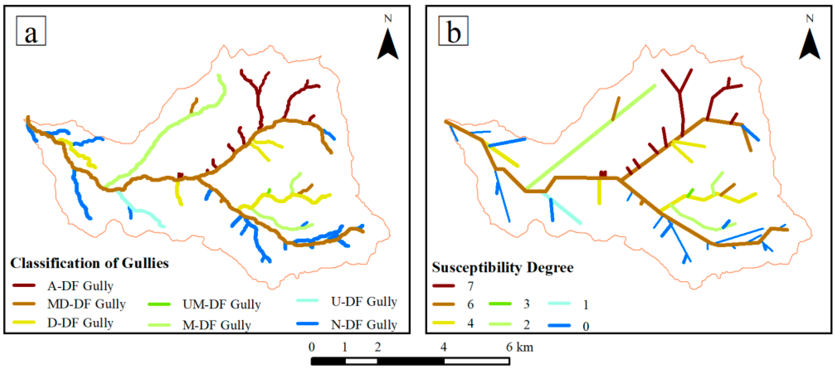
4.3. Classification of Debris Flow Gullies in the JJG and SD Marking

The different gully levels were superimposed and integrated with the recognized occurrence of debris flow (Figure 10a). For the different gully levels, the classification of debris flow gullies is proposed according to the classification methods mentioned above (Table 3). As it can be seen from Figure 10, the main gully belongs to the MD-DF gully, showing that debris flow occurs in the middle and down sections of the gully. There are 21 first-level sub-gullies in which the D-DF, MD-DF and A-DF gullies account for a large proportion, except the N-DF gullies. Different from the first-level sub-gullies in the JJG, the proportion of A-DF gullies in the second-level sub-gullies is particularly high, except the N-DF gullies. Because of the high hazard of the A-DF gullies, more attention should be paid to the prevention of debris flows in second-level sub-gullies. The number and type of the third-level gullies are relatively small, only including N-DF and A-DF gullies. Different gullies have different SDs. After simplifying the shape of the gullies in the JJG, different SDs for the debris flows were given in order to obtain the SD topological diagram of the debris flow gullies (Figure 10b).

4.4. HI and SE Values of Different Gullies

Using “Hypsometry Tools”, we can obtain the hypsometric curves and HI values for the topographic condition of the different gully levels. According to the geomorphic development stages put forward by Strahler [60], it can be demonstrated that the watershed of the main gully belongs to the mature stage (Figure 11a). Most of the watersheds corresponding to the first-level gullies also belong to the mature stage (Figure 11b). For the watersheds corresponding to the second-level gullies, half of the watersheds belong to the mature stage, and the other half belong to the young stage (Figure 11c). The watersheds corresponding to the third-level gullies are fewer, and the watersheds in the geomorphic mature stage account for 2/3 (Figure 11d). At the same time, we can see that a large number of watersheds in the Menqian Gully area in the north of the JJG belong to the young stage of geomorphic development (Figure 11e), which could provide better energy conditions for the development of debris flows.
According to the SE values for the material source conditions of the different watershed levels (Figure 12), the following could be demonstrated:
(1)
The whole JJG has a medium exposure (Figure 12a). It shows that the ecological environment of the JJG needs to be further improved. Measures such as returning farmland to forest and grassland, and planting trees and grass in bare land areas, need to be strengthened.
(2)
The land surfaces of a large number of watersheds in the Menqian Gully area in the north of the JJG show medium exposure (Figure 12b), which could provide better source conditions for the development of debris flows.
(3)
The vegetation condition of some gullies in the north is particularly poor (Figure 12c), meaning that it is very easy to provide a solid source supply for debris flow hazards.
(4)
The number of third-level sub-gullies is small, but this also shows the characteristics of good vegetation in the north and bad vegetation in the south (Figure 12d).
(5)
Through the superposition display of the exposed results of the different gully levels (the main gully is at the bottom), it could be found that the vegetation condition in the north is better than that in the south, and that there is a medium exposure characteristic for the whole gully (Figure 12e).

5. Discussion

5.1. Relationships betwween Landform and Different Debris Flow Gullies

A number of studies have shown the influence of watershed topography on the development of debris flow hazards [67,68], and have found that the watersheds with higher HI values for their topographic condition are more likely to have debris flows. This is because the gullies with higher HI values are steeper, and can provide more energy conditions for the development of debris flows. For an assessment of the susceptibility and hazard of debris flows on the watershed scale, we need to consider that the indicators need to better reflect the overall characteristics of watersheds. Compared to the topographic feature factors, such as the gully bed slope, the HI value of the watershed can reflect the overall topographic features of the watershed better and tell people whether the watershed is in the active stage of geomorphic development [69,70]. Cheng, Cui, Su, Jia and Choi [36] once studied the Mocoa debris flow disaster event, and found that the HI value of the watershed in which the disaster occurred was 0.49, reflecting the fact that the watershed was in the mature stage of landform development, and that the water and soil migration caused by mountain hazards was an important driving force for the developing of the watershed landform.
In order to explore the relationship between HIs and SDs, we drew a point graph (Figure 13). It can be seen that with the increase in HIs, the SD of debris flow gullies begin to increase. Because different SDs correspond to different types of debris flow gullies, it also shows that with the increase in HI values, the type of debris flow gully also changes significantly, especially towards the A-DF-gully (with SD as 7) debris flow gullies. However, we also need to realize that although there is a positive relationship between HIs and SDs, the relationship between them is not a strong correlation. The main reason is that the factors that affect the occurrence of debris flows are diverse, and they are agglutinating and interacting with each other, becoming a complex disaster system [71]. This is not to say that it is meaningless to study the relationship between HIs and SDs, because the geomorphic factors represented by HI are an important link in the occurrence of debris flows; in addition, the ways in which geomorphic factors affect the movement state of debris flows needs further in-depth consideration by the relevant scholars and in their disaster simulation research [72].

5.2. Relationships betwween Vegetation and Different Debris Flow Gullies

There are many factors that affect the development of debris flow gullies, and landform is only one factor. Vegetation coverage is another important factor affecting the development of debris flow [73]. First of all, vegetation can reduce the hydrodynamic conditions of debris flow formation. The canopy, stem and root of vegetation can partly intercept rainfall, reduce surface runoff and slow down the runoff confluence speed, so as to increase the confluence time and reduce the flood flow. The more luxuriant the branches and leaves are, the greater the interception effect is. In addition, vegetation plays an important role in controlling the solid material supply of debris flows. The trunk and root system can intercept some loose deposits on the slope and reduce the supply of debris flows [74]. Therefore, the destruction of forest vegetation is an important reason for the occurrence of catastrophic debris flows [36]. Many scholars have also considered various factors in terms of material supply. For example, geological and lithological conditions are important factors to be considered. However, it is not difficult to find that geological and lithological conditions would first act on the occurrence of landslides, and then the landslide deposits may become the source conditions of debris flows [75]. Therefore, geological and lithological conditions, as underground factors, indirectly cause the occurrence of debris flows. Maybe it would be a good choice to use SEs to measure the supply conditions of debris flows.
It can be demonstrated that there is a positive correlation between SE values and SDs. SEs can provide abundant material source conditions for debris flow. At the same time, when encountering rainfall, the hysteresis effect on water is weakened, which is conducive to the formation of confluence. These promoting effects on debris flow have been confirmed by some researchers [66,76]. Through this study, we can find that with the increase in SE values, the type of debris flow gully changes significantly, especially towards the A-DF-gully (with SD as 7) debris flow gullies (Figure 14). Similarly, affected by the complex system of debris flow disasters, although SEs and SDs also show a positive correlation, this relationship is not a strong correlation. However, this non-random relationship can also make us realize the role of vegetation in debris flows, and guide us to pay attention to the impact of vegetation in debris flow simulation [77].

5.3. Susceptibility Assessment Model Construction

As a complex disaster system, it is very difficult to evaluate the susceptibility and hazard of debris flow using only one influencing factor. However, increasing the number of factors and the calculation ability is a way of solving the problem of debris flow disaster assessment [78]. On the other hand, finding fewer and more critical factors is another solution and the key to the assessment of debris flow disasters, and it could simplify complex problems effectively [22]. In terms of debris flow formation, terrain, water source and material source are the three most direct conditions for the formation of debris flow hazards. The relationship between them is more obvious especially in the post-fire debris flow hazards [40]. Without considering the water source condition brought by rainfall, we studied the relationship between the SDs and the two factors (HIs and SEs). It can be seen that the SDs of debris flow gullies increase with the increase in SEs and HIs (Figure 15). This means that the types of gullies are also changing.
With the help of statistical software, we try to build a surface (Figure 15) to fit these three-dimensional points, and obtain the corresponding mathematical model (SD = −11.17 + 28.52 × SE + 20.60 × HI − 28.82 × SE2 − 5.69 × HI2). In the valley with low SEs and low HIs, there is basically no debris flow, while in the valley with high SE and high HI values, there is an A-DF debris flow gully. Comparing the better goodness-of-fit (R2 = 0.56), it could be found that the goodness-of-fit obtained by using HIs and SEs at the same time is better than that obtained by using only one factor (R2 is 0.25 and 0.37, respectively). This shows that the debris flow is the result of the interaction of many factors. We also need to recognize that the R2 value of the model is 0.56, which still has the possibility of further improvement.
In order to verify the validity of the model construction method, we used 70% of the data to rebuild the model, and the remaining 30% of the data as the validation data, and obtained the new model (SD = −11.4126 + 30.6035 × SE + 37.6692 × HI − 30.906 × SE2 − 20.2534 × HI2, R2 = 0.6219, p < 0.0001). We substituted the validation data into this model. If the calculated result was equal to or close to the defined SD value, the identification was considered valid. After calculation, the effective rate of identification reached 57%. Considering the different quantities of data, the models built were also different. In addition, the regional differences in the geographical environment was also considered [79]. Therefore, when the above susceptibility degree calculation model was used in practice, it was better to conduct resampling training to generate a local susceptibility calculation model. We also needed to realize that the use of such models is only applicable to the rapid and simple identification of the debris flow susceptibility degree and the debris flow gully type approximately.

6. Conclusions

(1)
According to the location of the debris flow occurring in each gully, there are different classifications of debris flow gullies. Different debris flow gullies have different characteristics and hence different corresponding SDs.
(2)
After clarifying the classification and nomenclature of different debris flow gullies, researchers could obtain a general understanding of debris flow gullies from their name. It should be noted that the gullies known as debris flow gullies not always represent a hazard everywhere.
(3)
A topological diagram of the debris flow gullies could be obtained after naming the different gully levels, assigning different SDs and simplifying the shape of the gullies. The topological diagram shows the different types of debris flow in the gullies using a more intuitive and simple way of expression. On the other hand, the topological setting of the debris flow gullies shows the relationship between the different types of debris flow gullies.
(4)
The debris flow classification method proposed by us can establish a good relationship with the HI and SE. We have proposed an SD assessment model construction method. Researchers can refer to this method in order to establish their own regional adaptability model for the assessment of the degree of debris flow gully susceptibility.
We hope that our research can provide a new concept for debris flow gullies. Our research on the classifications of debris flow gullies could contribute to the investigation of debris flow gullies. At the same time, this SD assessment model relates the assessment results with the different types of debris flow gully, which is also an innovation of this study.

Author Contributions

D.C. and C.G. designed the method and conceived the study plan; D.C. performed the calculation and analyzed the data; D.C., C.G. and J.I. wrote the paper. All authors have read and agreed to the published version of the manuscript.

Funding

This research was supported by the Research Topics of Henan Social Science Federation (reference number SKL-2022-2717), and the Research Start-up Fund of Henan University (reference number CX3050A0970209).

Data Availability Statement

Publicly available datasets were used in this study, and we have added the relevant data URL in the references.

Acknowledgments

The authors would like to thank the editors and the anonymous reviewers, as well as the colleagues, who gave them help in this study.

Conflicts of Interest

The authors declare no conflict of interest.

References

  1. Lanza, N.L.; Meyer, G.A.; Okubo, C.H.; Newsom, H.E.; Wiens, R.C. Evidence for debris flow gully formation initiated by shallow subsurface water on Mars. Icarus 2010, 205, 103–112. [Google Scholar] [CrossRef]
  2. Cannon, S.H.; Kirkham, R.M.; Parise, M. Wildfire-related debris-flow initiation processes, Storm King Mountain, Colorado. Geomorphology 2001, 39, 171–188. [Google Scholar] [CrossRef]
  3. Legg, N.T.; Meigs, A.J.; Grant, G.E.; Kennard, P. Debris flow initiation in proglacial gullies on Mount Rainier, Washington. Geomorphology 2014, 226, 249–260. [Google Scholar] [CrossRef]
  4. Chen, N.; Liu, M.; Liu, L. A discussion on how to discriminate the hazard and watershed properties of mountain torrent and debris Flow. Flow J. Catastrophol. 2018, 33, 39–43. [Google Scholar]
  5. Shen, W.; Li, T.; Li, P.; Lei, Y. Numerical assessment for the efficiencies of check dams in debris flow gullies: A case study. Comput. Geotech. 2020, 122, 103541. [Google Scholar] [CrossRef]
  6. Jackson, L.E., Jr.; Kostaschuk, R.A.; Macdonald, G.M. Identification of debris flow hazard on alluvial fans in the Canadian Rocky Mountains. GSA Rev. Eng. Geol. 1984, 7, 115–124. [Google Scholar]
  7. Sinha, R.K.; Vijayan, S.; Shukla, A.D.; Das, P.; Bhattacharya, F. Gullies and debris-flows in Ladakh Himalaya, India: A potential Martian analogue. Geol. Soc. Lond. Spec. Publ. 2019, 467, 315–342. [Google Scholar] [CrossRef]
  8. Jakob, M.; Hungr, O.; Jakob, D.M. Debris-Flow Hazards and Related Phenomena; Springer: Berlin/Heidelberg, Germany, 2005; Volume 739. [Google Scholar]
  9. Zhong, D.; Yang, Q.; Yang, R. Debris flows in Northeast China. J. Mt. Res. 1984, 2, 36–42. [Google Scholar]
  10. Nistor, C.J.; Church, M. Suspended sediment transport regime in a debris-flow gully on Vancouver Island, British Columbia. Hydrol. Process. Int. J. 2005, 19, 861–885. [Google Scholar] [CrossRef]
  11. Zhu, J. Judgement of Debris Flow Ravines and Evaluation of Risk Degree of Debris Flows. Arid Land Geogr. 1995, 18, 63–71. [Google Scholar]
  12. Tang, C.; Zhu, J.; Li, W.; Liang, J. Rainfall-triggered debris flows following the Wenchuan earthquake. Bull. Eng. Geol. Environ. 2009, 68, 187–194. [Google Scholar] [CrossRef]
  13. Liu, Y.; Guo, H.C.; Zou, R.; Wang, L.J. Neural network modeling for regional hazard assessment of debris flow in Lake Qionghai Watershed, China. Environ. Geol. 2005, 49, 968–976. [Google Scholar] [CrossRef]
  14. Cao, C.; Xu, P.; Chen, J.; Zheng, L.; Niu, C. Hazard Assessment of Debris-Flow along the Baicha River in Heshigten Banner, Inner Mongolia, China. Int. J. Environ. Res. Public Health 2016, 14, 30. [Google Scholar] [CrossRef] [Green Version]
  15. Hollingsworth, R.; Kovacs, G. Soil slumps and debris flows: Prediction and protection. Bull. Assoc. Eng. Geol. 1981, 18, 17–28. [Google Scholar] [CrossRef]
  16. Zhang, W.; Li, H.-Z.; Chen, J.-P.; Zhang, C.; Xu, L.-M.; Sang, W.-F. Comprehensive hazard assessment and protection of debris flows along Jinsha River close to the Wudongde dam site in China. Nat. Hazards 2011, 58, 459–477. [Google Scholar] [CrossRef]
  17. Chen, J.; Li, Y.; Zhou, W.; Iqbal, J.; Cui, Z. Debris-Flow Susceptibility Assessment Model and Its Application in Semiarid Mountainous Areas of the Southeastern Tibetan Plateau. Nat. Hazards Rev. 2017, 18, 05016005. [Google Scholar] [CrossRef]
  18. Tie, Y.; Tang, C.; Zhou, C. Information entropy-based hazard assessment of debris flow gully in Dongchuan urban area of Kunming City. Chin. J. Geol. Hazard Control 2006, 17, 80–82. [Google Scholar]
  19. Tie, Y.; Tang, C. Application of AHP in single debris flow risk assessment. Chin. J. Geol. Hazard Control 2006, 17, 79–84. [Google Scholar]
  20. Liu, X.; Tang, C.; Zhang, S. Quantitative judgment on the debris flow risk degree. J. Catastrophol. 1993, 8, 1–7. [Google Scholar]
  21. Jiang, H.; Zou, Q.; Zhou, B.; Hu, Z.; Li, C.; Yao, S.; Yao, H. Susceptibility Assessment of Debris Flows Coupled with Ecohydrological Activation in the Eastern Qinghai-Tibet Plateau. Remote Sens. 2022, 14, 1444. [Google Scholar] [CrossRef]
  22. Cui, Y.; Cheng, D.; Chan, D. Investigation of post-fire debris flows in Montecito. ISPRS Int. J. Geo-Inf. 2018, 8, 5. [Google Scholar] [CrossRef] [Green Version]
  23. Wang, Y.; Zhan, Q.; Tian, B.; Hong, Y.; Zou, R. The relationship between the variation of annual rainfall and the variation of sedi-ment transport by debris flows at Jiangjia Gully in the upper reach of Yangtze River. J. Mt. Sci. 2008, 26, 590–596. [Google Scholar]
  24. Zhuang, J.; Cui, P.; Wang, G.; Chen, X.; Iqbal, J.; Guo, X. Rainfall thresholds for the occurrence of debris flows in the Jiangjia Gully, Yunnan Province, China. Eng. Geol. 2015, 195, 335–346. [Google Scholar] [CrossRef]
  25. Tian, X.; Su, F.; Guo, X.; Liu, J.; Li, Y. Material sources supplying debris flows in Jiangjia Gully. Environ. Earth Sci. 2020, 79, 318. [Google Scholar]
  26. Chen, J.; He, Y.; Wei, F. Debris flow erosion and deposition in Jiangjia Gully, Yunnan, China. Environ. Geol. 2005, 48, 771–777. [Google Scholar] [CrossRef]
  27. Li, Y.; Liu, J.; Su, F.; Xie, J.; Wang, B. Relationship between grain composition and debris flow characteristics: A case study of the Jiangjia Gully in China. Landslides 2015, 12, 19–28. [Google Scholar] [CrossRef]
  28. Guo, X.; Li, Y.; Cui, P.; Yan, H.; Zhuang, J. Intermittent viscous debris flow formation in Jiangjia Gully from the perspectives of hydrological processes and material supply. J. Hydrol. 2020, 589, 125184. [Google Scholar] [CrossRef]
  29. Peng, H.; Zhao, Y.; Cui, P.; Zhang, W.; Chen, X.; Chen, X. Two-dimensional numerical model for debris flows in the Jiangjia Gully, Yunnan Province. J. Mt. Sci. 2011, 8, 757–766. [Google Scholar] [CrossRef]
  30. Lamsal, D.; Sawagaki, T.; Watanabe, T. Digital terrain modelling using Corona and ALOS PRISM data to investigate the distal part of Imja Glacier, Khumbu Himal, Nepal. J. Mt. Sci. 2011, 8, 390–402. [Google Scholar] [CrossRef] [Green Version]
  31. Bouvet, M.; Goryl, P.; Chander, G.; Santer, R.; Saunier, S. Preliminary radiometric calibration assessment of ALOS AVNIR-2. In Proceedings of the 2007 IEEE International Geoscience and Remote Sensing Symposium, Barcelona, Spain, 23–28 July 2007; pp. 2673–2676. [Google Scholar]
  32. Rignot, E. Changes in West Antarctic ice stream dynamics observed with ALOS PALSAR data. Geophys. Res. Lett. 2008, 35, L12505. [Google Scholar] [CrossRef] [Green Version]
  33. ASF Data Search. Available online: https://search.asf.alaska.edu/#/?dataset=ALOS&productTypes=ALOS$$&beamModes=ALOS$$&polarizations=ALOS$$&flightDirs= (accessed on 17 August 2019).
  34. Lisle, R.J. Google Earth: A new geological resource. Geol. Today 2010, 22, 29–32. [Google Scholar] [CrossRef]
  35. Cheng, D.; Gao, C.; Shao, T.; Iqbal, J. A Landscape Study of Sichuan University (Wangjiang Campus) from the Perspective of Campus Tourism. Land 2020, 9, 499. [Google Scholar] [CrossRef]
  36. Cheng, D.; Cui, Y.; Su, F.; Jia, Y.; Choi, C.E. The characteristics of the Mocoa compound disaster event, Colombia. Landslides 2018, 15, 1223–1232. [Google Scholar] [CrossRef] [Green Version]
  37. Cheng, D.; Cui, Y.; Li, Z.; Iqbal, J. Watch Out for the Tailings Pond, a Sharp Edge Hanging over Our Heads: Lessons Learned and Perceptions from the Brumadinho Tailings Dam Failure Disaster. Remote Sens. 2021, 13, 1775. [Google Scholar] [CrossRef]
  38. Wikipedia. Landsat 8. Available online: https://en.wikipedia.org/wiki/Landsat_8 (accessed on 8 July 2019).
  39. USGS, GloVis. Available online: https://glovis.usgs.gov/ (accessed on 21 July 2019).
  40. Xiong, K.; Adhikari, B.R.; Stamatopoulos, C.A.; Zhan, Y.; Wu, S.; Dong, Z.; Di, B. Comparison of different machine learning methods for debris flow susceptibility mapping: A case study in the Sichuan Province, China. Remote Sens. 2020, 12, 295. [Google Scholar] [CrossRef] [Green Version]
  41. Liang, W.-J.; Zhuang, D.-F.; Jiang, D.; Pan, J.-J.; Ren, H.-Y. Assessment of debris flow hazards using a Bayesian Network. Geomorphology 2012, 171, 94–100. [Google Scholar] [CrossRef]
  42. Elkadiri, R.; Sultan, M.; Youssef, A.M.; Elbayoumi, T.; Chase, R.; Bulkhi, A.B.; Al-Katheeri, M.M. A remote sensing-based approach for debris-flow susceptibility assessment using artificial neural networks and logistic regression modeling. IEEE J. Sel. Top. Appl. Earth Obs. Remote Sens. 2014, 7, 4818–4835. [Google Scholar] [CrossRef]
  43. Heathcote, I.W. Integrated Watershed Management: Principles and Practice; John Wiley & Sons: Hoboken, NJ, USA, 2009. [Google Scholar]
  44. Tebano, C.; Pasanisi, F.; Grauso, S. QMorphoStream: Processing tools in QGIS environment for the quantitative geomorphic analysis of watersheds and river networks. Earth Sci. Inform. 2017, 10, 257–268. [Google Scholar] [CrossRef]
  45. Gao, C.; Cheng, D.; Iqbal, J.; Yao, S. Spatiotemporal Change Analysis and Prediction of the Great Yellow River Region (GYRR) Land Cover and the Relationship Analysis with Mountain Hazards. Land 2023, 12, 340. [Google Scholar] [CrossRef]
  46. Olaya, V.; Conrad, O. Geomorphometry in SAGA. Dev. Soil Sci. 2009, 33, 293–308. [Google Scholar]
  47. Jenkins, D.G.; McCauley, L.A. GIS, SINKS, FILL, and disappearing wetlands: Unintended consequences in algorithm development and use. In Proceedings of the 2006 ACM Symposium on Applied Computing, Dijon, France, 23–27 April 2006; pp. 277–282. [Google Scholar]
  48. Lindsay, J.B. Efficient hybrid breaching-filling sink removal methods for flow path enforcement in digital elevation models. Hydrol. Process. 2016, 30, 846–857. [Google Scholar] [CrossRef]
  49. Omran, A.; Dietrich, S.; Abouelmagd, A.; Michael, M. New ArcGIS tools developed for stream network extraction and basin delineations using Python and java script. Comput. Geosci. 2016, 94, 140–149. [Google Scholar] [CrossRef]
  50. Schäuble, H.; Marinoni, O.; Hinderer, M. A GIS-based method to calculate flow accumulation by considering dams and their specific operation time. Comput. Geosci. 2008, 34, 635–646. [Google Scholar] [CrossRef]
  51. Qin, C.-Z.; Zhan, L. Parallelizing flow-accumulation calculations on graphics processing units—From iterative DEM preprocessing algorithm to recursive multiple-flow-direction algorithm. Comput. Geosci. 2012, 43, 7–16. [Google Scholar] [CrossRef]
  52. Xiong, J.; Wei, F.; Liu, Z. Hazard assessment of debris flow in Sichuan Province. J. Geo-Inf. Sci 2017, 19, 1604–1612. [Google Scholar]
  53. Horton, R.E. Erosional development of streams and their drainage basins; hydrophysical approach to quantitative morphology. Geol. Soc. Am. Bull. 1945, 56, 275–370. [Google Scholar] [CrossRef] [Green Version]
  54. Liu, S.M.; Zhang, J.; Chen, H.; Wu, Y.; Xiong, H.; Zhang, Z. Nutrients in the Changjiang and its tributaries. Biogeochemistry 2003, 62, 1–18. [Google Scholar] [CrossRef]
  55. Liu, C.-N.; Huang, H.-F.; Dong, J.-J. Impacts of September 21, 1999 Chi-Chi earthquake on the characteristics of gully-type debris flows in central Taiwan. Nat. Hazards 2008, 47, 349–368. [Google Scholar] [CrossRef]
  56. Chevalier, G.G.; Medina, V.; Hürlimann, M.; Bateman, A. Debris-flow susceptibility analysis using fluvio-morphological parameters and data mining: Application to the Central-Eastern Pyrenees. Nat. Hazards 2013, 67, 213–238. [Google Scholar] [CrossRef]
  57. Wei, F.; Hu, K.; Lopez, J. Debris-flow risk zoning and its application in disaster mitigation. Chin. J. Geol. Hazard Control. 2007, 18, 22–27. [Google Scholar]
  58. Zhang, S.; Zhang, J.; Zhang, B. Deduction and application of generalized Euler formula in topological relation of geographic information system (GIS). Sci. China Ser. D Earth Sci. 2004, 47, 749–759. [Google Scholar] [CrossRef]
  59. Delafontaine, M.; Van de Weghe, N.; Bogaert, P.; De Maeyer, P. Qualitative relations between moving objects in a network changing its topological relations. Inf. Sci. 2008, 178, 1997–2006. [Google Scholar] [CrossRef]
  60. Strahler, A.N. Hypsometric (area-altitude) analysis of erosional topography. Geol. Soc. Am. Bull. 1952, 63, 1117–1142. [Google Scholar] [CrossRef]
  61. Davis, J. Hypsometry Tools Instructions. Available online: https://gis.sfsu.edu/content/hypsometry-tools (accessed on 4 January 2020).
  62. Mu, S.; Li, J.; Chen, Y.; Gang, C.; Zhou, W.; Ju, W. Spatial Differences of Variations of Vegetation Coverage in Inner Mongolia during 2001–2010. Acta Geogr. Sin. 2012, 67, 1255–1268. [Google Scholar] [CrossRef]
  63. Carlson, T.N.; Ripley, D.A. On the relation between NDVI, fractional vegetation cover, and leaf area index. Remote Sens. Environ. 1997, 62, 241–252. [Google Scholar] [CrossRef]
  64. Rundquist, B.C. The influence of canopy green vegetation fraction on spectral measurements over native tallgrass prairie. Remote Sens. Environ. 2002, 81, 129–135. [Google Scholar] [CrossRef]
  65. Maurer, T. How to pan-sharpen images using the gram-schmidt pan-sharpen method–A recipe. In Proceedings of the ISPRS Hannover Workshop 2013, Hannover, Germany, 21–24 May 2013; International Archives of the Photogrammetry, Remote Sensing and Spatial Information Sciences: Hannover, Germany, 2013; Volume XL-1/W1. [Google Scholar]
  66. Cui, Y.; Cheng, D.; Choi, C.E.; Jin, W.; Lei, Y.; Kargel, J.S. The cost of rapid and haphazard urbanization: Lessons learned from the Freetown landslide disaster. Landslides 2019, 16, 1167–1176. [Google Scholar] [CrossRef] [Green Version]
  67. Li, Y.; Hu, K.; Su, F.; Su, P. Debris flow viewed from the basin evolution—A case study of Jiangjia Gulley, Yunnan. J. Mt. Sci. 2009, 27, 449–456. [Google Scholar]
  68. Xiang, L.; Li, Y.; Chen, H.; Su, F.; Huang, X. Sensitivity analysis of debris flow along highway based on geomorphic evolution theory. Resour. Environ. Yangtze Basin 2015, 24, 1984–1992. [Google Scholar]
  69. Gallen, S.F.; Wegmann, K.W.; Frankel, K.L.; Hughes, S.; Lewis, R.Q.; Lyons, N.; Paris, P.; Ross, K.; Bauer, J.B.; Witt, A.C. Hillslope response to knickpoint migration in the Southern Appalachians: Implications for the evolution of post-orogenic landscapes. Earth Surf. Process. Landf. 2011, 36, 1254–1267. [Google Scholar] [CrossRef]
  70. Singh, O.; Sarangi, A.; Sharma, M.C. Hypsometric integral estimation methods and its relevance on erosion status of north-western lesser Himalayan watersheds. Water Resour. Manag. 2008, 22, 1545–1560. [Google Scholar] [CrossRef]
  71. Kung, H.-Y.; Chen, C.-H.; Ku, H.-H. Designing intelligent disaster prediction models and systems for debris-flow disasters in Taiwan. Expert Syst. Appl. 2012, 39, 5838–5856. [Google Scholar] [CrossRef]
  72. Zhou, J.-W.; Cui, P.; Yang, X.-G. Dynamic process analysis for the initiation and movement of the Donghekou landslide-debris flow triggered by the Wenchuan earthquake. J. Asian Earth Sci. 2013, 76, 70–84. [Google Scholar] [CrossRef]
  73. Gabet, E.J.; Dunne, T. Landslides on coastal sage-scrub and grassland hillslopes in a severe El Niño winter: The effects of vegetarian conversion on sediment delivery. Geol. Soc. Am. Bull. 2002, 114, 983–990. [Google Scholar] [CrossRef]
  74. Istanbulluoglu, E.; Tarboton, D.G.; Pack, R.T.; Luce, C.H. Modeling of the interactions between forest vegetation, disturbances, and sediment yields. J. Geophys. Res. Earth Surf. 2004, 109, F01009. [Google Scholar] [CrossRef] [Green Version]
  75. Cheng, D. Hazard Analysis of Mountain-Hazards in the Areas of the Silk Road Economic Belt; University of Chinese Academy of Sciences: Beijing, China, 2020. [Google Scholar]
  76. Wang, J.; Yang, H.; Ren, G.; Dong, L.I.; Zhang, T. Formation Condition and Activity Characteristics of Debris Flow for Coarse Grained Granite of Ragstone in Xinjiang. Water Resour. Power 2013, 31, 141–151. [Google Scholar]
  77. Shen, P.; Zhang, L.M.; Chen, H.; Gao, L. Role of vegetation restoration in mitigating hillslope erosion and debris flows. Eng. Geol. 2017, 216, 122–133. [Google Scholar] [CrossRef]
  78. Liang, Z.; Wang, C.-M.; Zhang, Z.-M.; Khan, K.-U.-J. A comparison of statistical and machine learning methods for debris flow susceptibility mapping. Stoch. Environ. Res. Risk Assess. 2020, 34, 1887–1907. [Google Scholar] [CrossRef]
  79. Cheng, D.; Gao, C. Regionalization Research of Mountain-Hazards Developing Environments for the Eurasian Continent. Land 2022, 11, 1519. [Google Scholar] [CrossRef]
Figure 1. Location of the JJG. (a) Location of Northeast Yunnan in China; (b) JJG’s location in Northeast Yunnan. (c) JJG watershed and its main river network.
Land 12 00571 g001
Figure 2. Data of the JJG. (a) DEM data of the JJG; (b) High-resolution remote sensing image of the JJG.
Land 12 00571 g002
Figure 3. Relationships of rainfall excitation conditions, topographic conditions and material source conditions in debris flow susceptibility and hazard assessment. When only susceptibility assessment is conducted, topographic and material source conditions are the main control factors, while the impact of the rainfall triggering factor should be considered when conducting the debris flow hazard assessment [25].
Land 12 00571 g003
Figure 4. Watershed extraction. (a) Generation of the sink-filling raster image; (b) Calculation of the flow direction raster image and construction of the flow accumulation raster image; (c) Generation of the river network and the gully line raster image, and drawing of the pour points and extraction of the watersheds.
Land 12 00571 g004
Figure 5. “Three-section method (TSM)” of debris flow gully classification. (a) Three sections of one gully, including U-S, M-S and D-S; (b) Debris flows in different sections of the first-level sub-gully; (c) Debris flows in different sections of the main gully. Some sections of gullies where debris flows occur are marked in brown. Considering the occurrences of debris flows at different locations in the gullies, eight combinations can be obtained.
Land 12 00571 g005
Figure 6. Technology roadmap.
Land 12 00571 g006
Figure 7. Division of main and sub-gullies in JJG and their confluence areas. (a) Main and sub-gullies; (b) Confluence area of the main gully; (c) Confluence area of the first-level sub-gully; (d) Confluence area of the second-level sub-gully; (e) Confluence area of the third-level sub-gully. The JJG includes 1 main gully, 21 first-level gullies, 21 second-level gullies and 3 third-level gullies.
Land 12 00571 g007
Figure 8. Examples of remote sensing image interpretation of debris flows. In the process of interpretation, the debris flow accumulation is an important symbol of interpretation. At the same time, the landslide mass on both sides of the gullies can provide rich material source conditions for the occurrence of debris flows, which can also provide important reference for the interpretation of debris flows.
Land 12 00571 g008
Figure 9. Identification of debris flow occurring in the gullies: (a) Identification results of debris flows; ①–④ Local enlargement pictures of high-resolution remote sensing images. The blue lines in the pictures are the gully lines.
Land 12 00571 g009
Figure 10. Gully classification and different susceptibility degrees. (a) Overlay display of the different gully levels and their classification; (b) Susceptibility degree topological diagram of debris flow gullies. We have not obtained UD-DF gullies (Digital ID = 5) in the JJG, but only seven of the eight categories were successfully interpreted.
Land 12 00571 g010
Figure 11. HI values of the different watershed levels. (a) Watershed of the main gully; (b) Watershed of the first-level sub-gully; (c) Watershed of the second-level sub-gully; (d) Watershed of the third-level sub-gully; (e) Overlay effect of each watershed.
Land 12 00571 g011
Figure 12. SE values of different watersheds corresponding to the different gully levels. (a) Watershed of the main gully; (b) Watershed of the first-level sub-gully; (c) Watershed of the second-level sub-gully; (d) Watershed of the third-level sub-gully; (e) Overlay effect of each watershed.
Land 12 00571 g012
Figure 13. Relationships between HIs and SDs. HIs represent the geomorphic development status of gullies, which are calculated quantitative values. SDs are the susceptibility level defined by us, which can be considered as semi-quantitative values. We use different colors to distinguish different types of debris flow gullies. According to the regression equation, with the increase in HIs, the SDs of debris flow gullies show an increasing trend, indicating that the gully is more likely to suffer from debris flows. The R2 of the fitting model of HIs and SDs is 0.25, and p is 0.002. The formula in the figure is only a result that we try to fit. Since there are no continuous values on the axes, it is not ruled out that there is a better fitting equation.
Land 12 00571 g013
Figure 14. Relationships between SEs and SDs. SEs represent the land surface exposure, which are calculated quantitative values. SDs are the susceptibility level defined by us, which can be considered as semi-quantitative values. We use different colors to distinguish the different types of debris flow gully. According to the regression equation, with the increase in SE, the SDs of debris flow gullies show an increasing trend, indicating that the gully is more likely to suffer from debris flows. The R2 of the fitting model of SEs and SDs is 0.37, with p < 0.001. Since there are no continuous values on the axes, it is not ruled out that there is a better fitting equation.
Land 12 00571 g014
Figure 15. Fitting relationship for SD, SE and HI values. SDs are the susceptibility level defined by us, which can be considered as semi-quantitative values. HIs represent the geomorphic development status of gullies, which are calculated quantitative values. SEs represent the land surface exposure, which are calculated quantitative values. R2 of fitting model is 0.56, with p < 0.001. There is a good slope trend based on the three variables. Since there are no-continuous values on the axes, it is not ruled out that there is a better fitting equation.
Land 12 00571 g015
Table 1. Landsat 8 remote sensing images used for the calculation of vegetation coverage [39].
File NameResolutionDate of Data Acquisition
LC08_L1TP_129042_20190507_20190521_01_T115 m/30 m/100 m (panchromatic/multispectral/thermal)21 May 2019
LC08_L1TP_129042_20190811_20190820_01_T115 m/30 m/100 m (panchromatic/multispectral/thermal)20 August 2019
Table 2. Classifications of debris flow gullies and definition of SDs.
Full NameAbbreviationMeaningSusceptibility Degree (Digital ID)
No Debris flow gullyN-DF Gully No debris flow occurred in the whole gully.0
Upper-section Debris flow gully U-DF GullyDebris flows occur in the upper section of a gully.1
Middle-section Debris flow gullyM-DF GullyDebris flows occur in the middle section of a gully.2
Upper-Middle-section Debris flow gullyUM-DF GullyDebris flows occur in the upper and middle sections of a gully.3 (1 + 2)
Down-section
Debris flow gully
D-DF GullyDebris flows occur in the down section of a gully.4
Upper-Down-section Debris flow gullyUD-DF GullyDebris flows occur in the upper and down sections of a gully.5 (1 + 4)
Middle-Down-section Debris flow gullyMD-DF GullyDebris flows occur in the middle and down sections of a gully.6 (2 + 4)
Upper-Middle-Down-section Debris flow gullyA-DF GullyDebris flows occur in all sections of a gully.7 (1 + 2 + 4)
Table 3. Statistics of different debris flow gullies in the JJG.
Level of GulliesClassifications of Debris Flow GulliesSusceptibility DegreeCount
Main GullyMD-DF Gully61
First-level Sub-gullyN-DF Gully012
U-DF Gully11
M-DF Gully21
D-DF Gully43
MD-DF Gully62
A-DF Gully72
Second-level Sub-gullyN-DF Gully07
M-DF Gully22
D-DF Gully42
UM-DF Gully31
MD-DF Gully62
A-DF Gully77
Third-level Sub-gullyN-DF Gully01
A-DF Gully72
Disclaimer/Publisher’s Note: The statements, opinions and data contained in all publications are solely those of the individual author(s) and contributor(s) and not of MDPI and/or the editor(s). MDPI and/or the editor(s) disclaim responsibility for any injury to people or property resulting from any ideas, methods, instructions or products referred to in the content.

