
Mapping Priority Areas for Connectivity of Yellow-Winged Darter (Sympetrum flaveolum, Linnaeus 1758) under Climate Change

 ,
,  , , , ,
  and
and 
Abstract
:1. Introduction
2. Material and Method
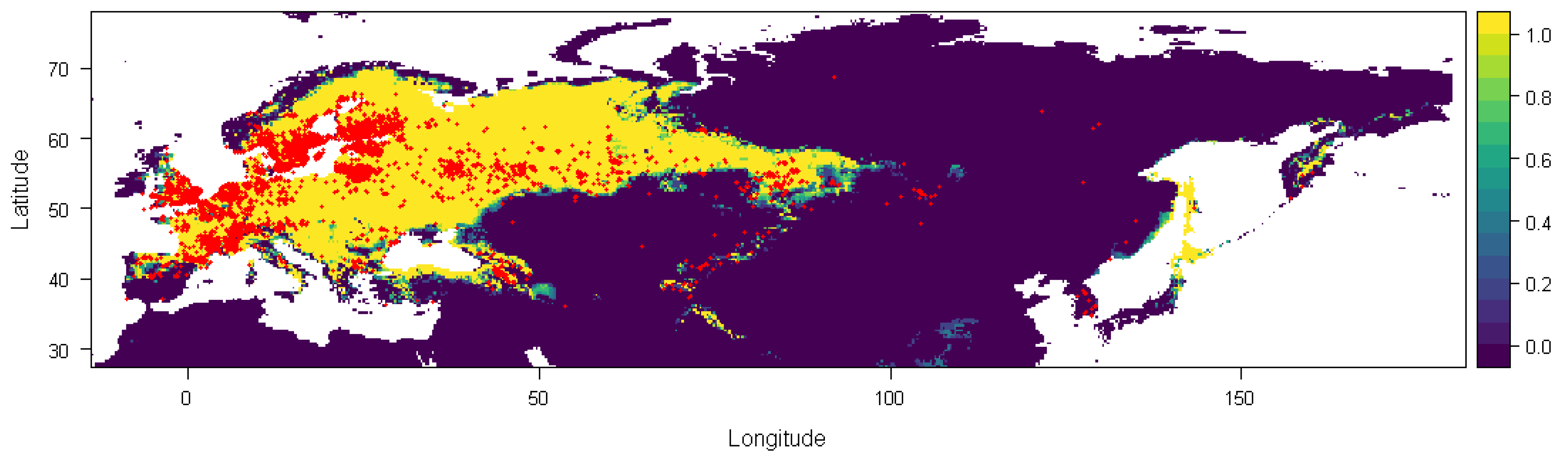
2.1. Species
2.2. Study Area
2.3. Occurrence Data
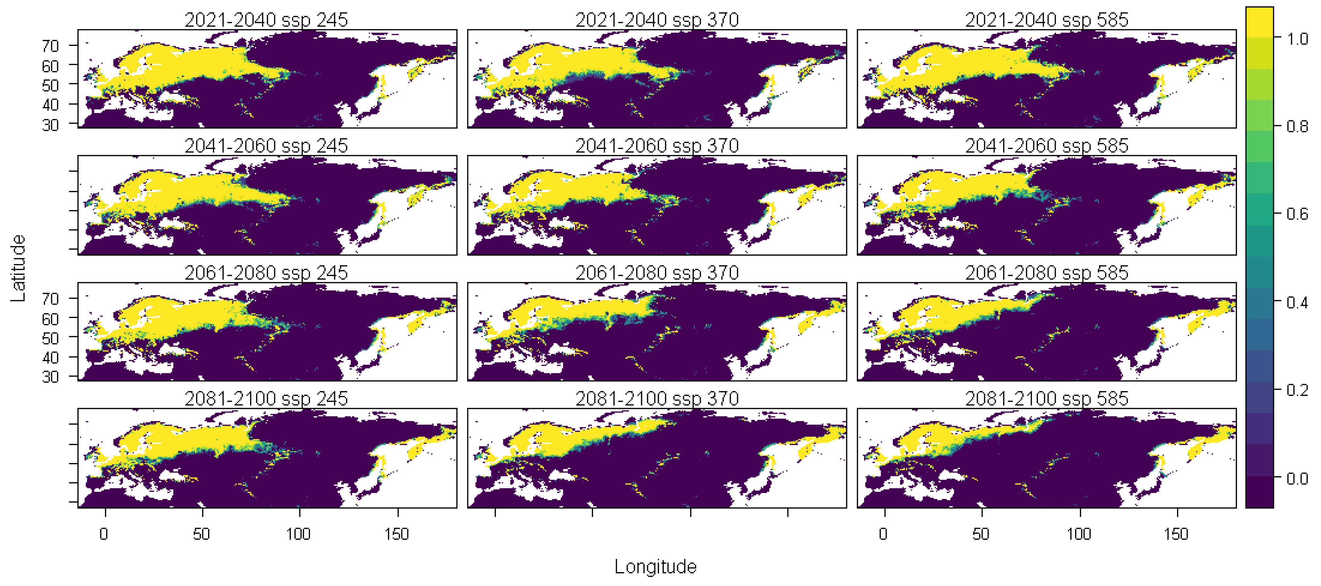
Climate Data
2.4. Methodology
2.5. Statistical Analysis
3. Results
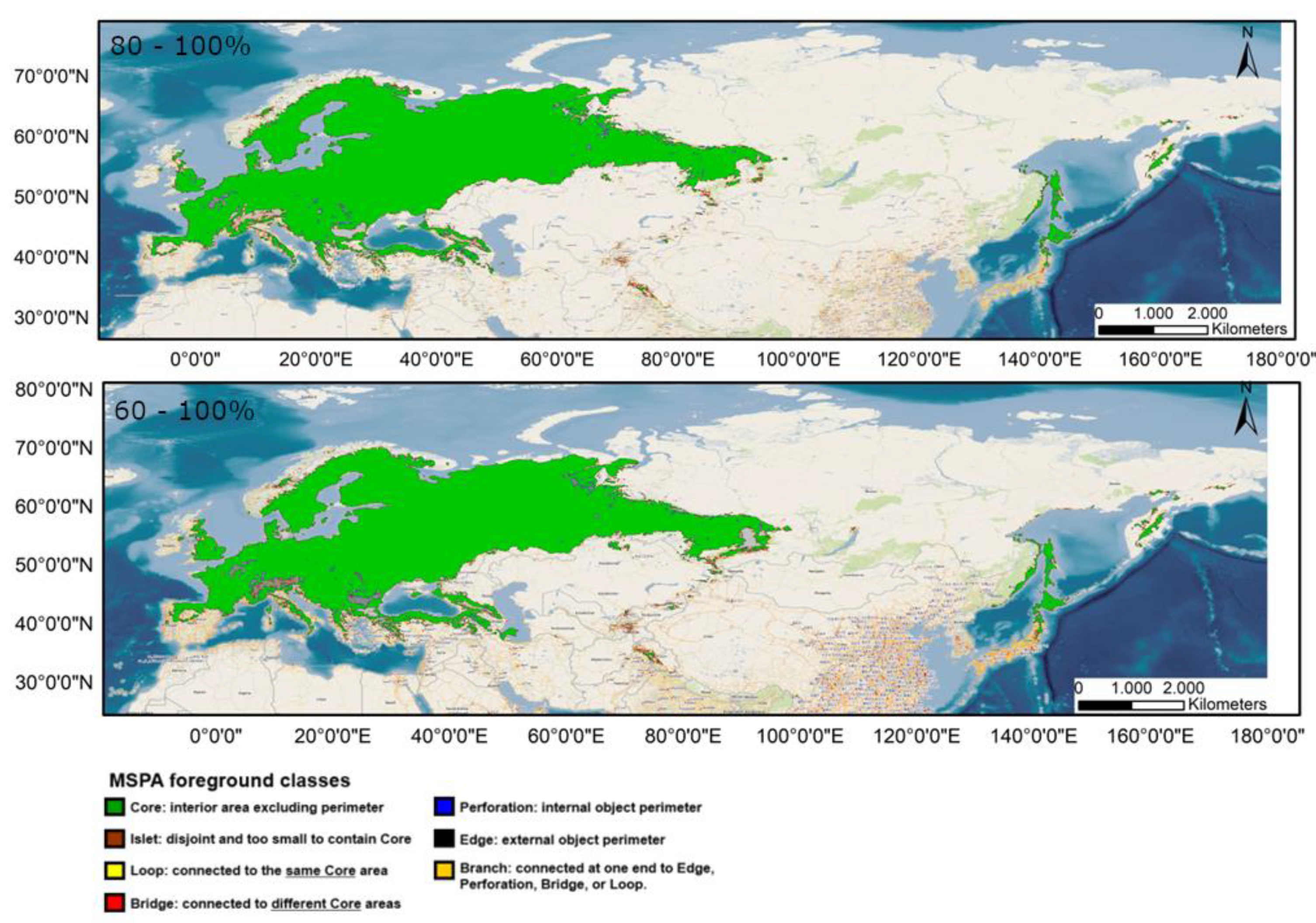
3.1. MSPA Index
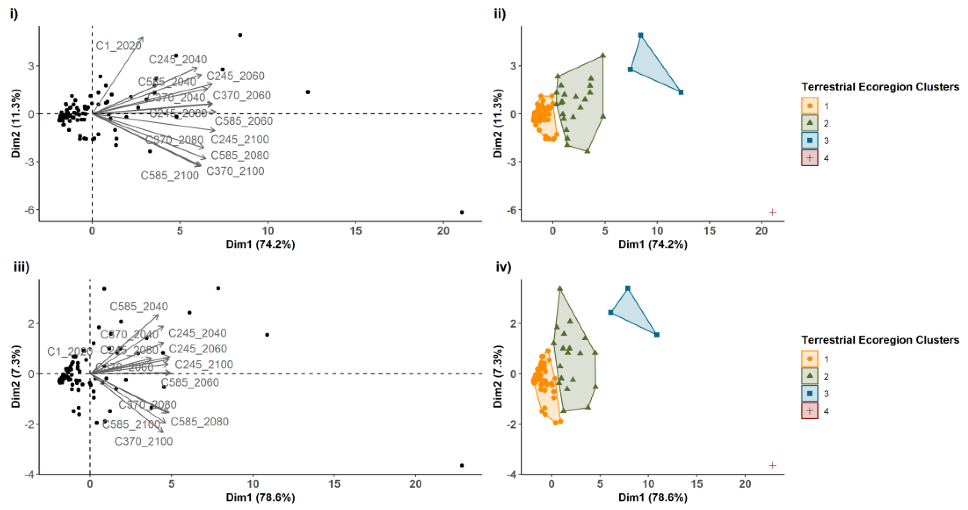
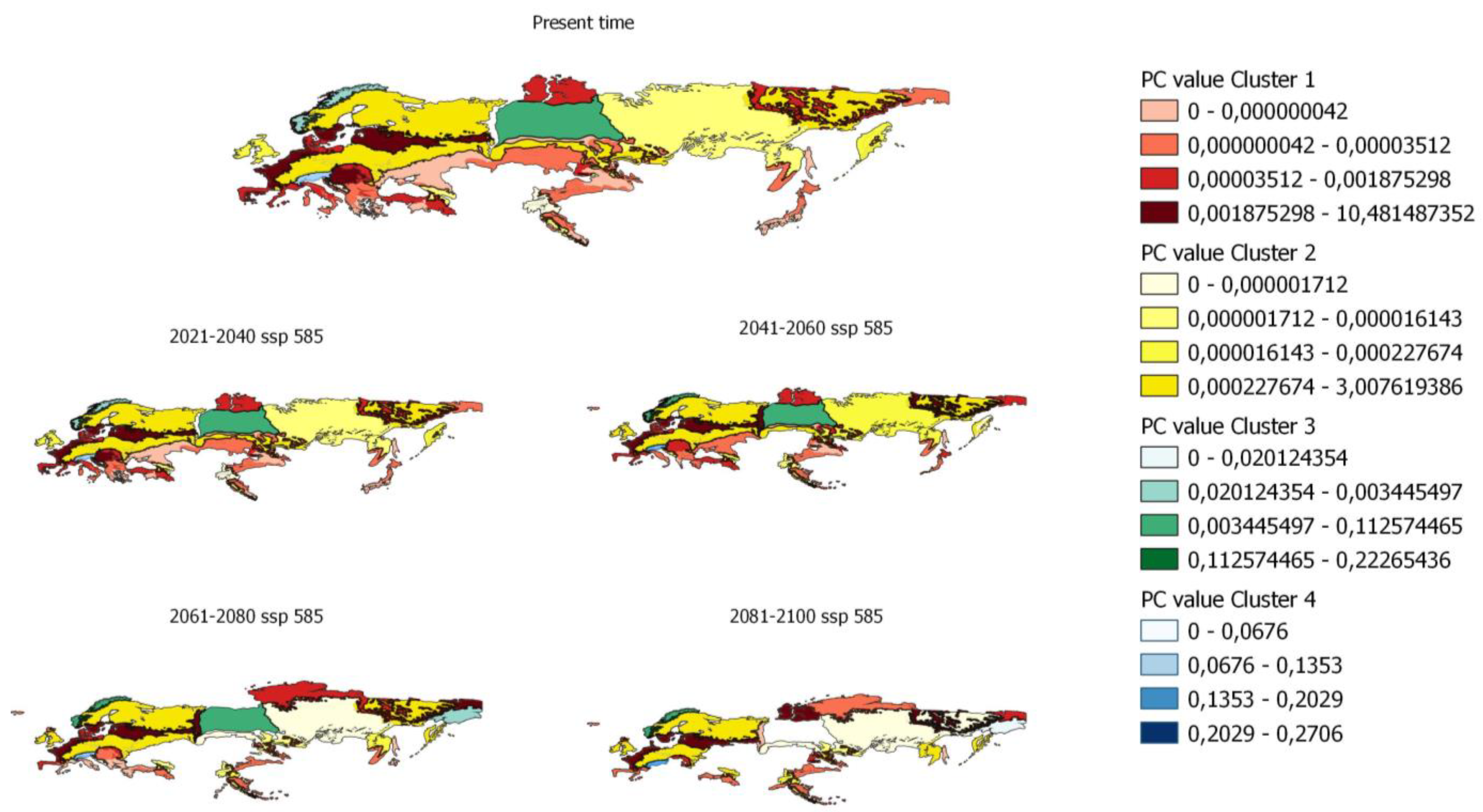
3.2. PC Index
4. Discussion
5. Conclusions
Author Contributions
Funding
Data Availability Statement
Conflicts of Interest
Appendix A
Appendix A.1. MSPA Analysis under Different Climate Scenarios (60–100%)
 |
 |
 |
 |
Appendix A.2. MSPA Analysis under Different Climate Scenarios (80–100%)
 |
 |
 |
 |
Appendix A.3. Critical Areas for Connectivity under Different Climate Scenarios (60–100%)
 |
 |
 |
Appendix A.4. Critical Areas for Connectivity under Different Climate Scenarios (80–100%)
 |
 |
 |
Appendix A.5. MSPA Analysis under Different Climate Scenarios (60–100%)
 |
 |
 |
Appendix A.6. MSPA Analysis under Different Climate Scenarios (80–100%)
 |
 |
 |
Appendix A.7. Cluster Calculation (60–100%)
| ECO_NAME | Terrestrial Ecoregion Clusters | C1_ 2020 | C245_2040 | C245_2060 | C245_2080 | C245_2100 | C370_2040 | C370_2060 | C370_2080 | C370_2100 | C585_2040 | C585_2060 | C585_2080 | C585_2100 |
| Aegean And Western Turkey Sclerophyllous And Mixed Forests | 1 | 53 | 3 | 5 | 0 | 0 | 2 | 0 | 0 | 0 | 2 | 0 | 0 | 0 |
| Alps Conifer And Mixed Forests | 4 | 0 | 466 | 601 | 674 | 836 | 671 | 747 | 867 | 832 | 526 | 812 | 949 | 810 |
| Altai Alpine Meadow And Tundra | 2 | 168 | 80 | 112 | 60 | 41 | 155 | 51 | 27 | 93 | 61 | 83 | 84 | 85 |
| Altai Montane Forest And Forest Steppe | 2 | 132 | 33 | 80 | 61 | 88 | 71 | 64 | 48 | 60 | 105 | 78 | 46 | 35 |
| Altai Steppe And Semi-Desert | 1 | 40 | 13 | 0 | 13 | 14 | 16 | 2 | 3 | 13 | 3 | 10 | 0 | 7 |
| Anatolian Conifer And Deciduous Mixed Forests | 1 | 124 | 25 | 2 | 4 | 8 | 0 | 4 | 10 | 2 | 9 | 4 | 2 | 0 |
| Appenine Deciduous Montane Forests | 1 | 5 | 57 | 39 | 44 | 25 | 60 | 22 | 0 | 0 | 47 | 28 | 5 | 0 |
| Atlantic Mixed Forests | 1 | 10 | 38 | 95 | 26 | 29 | 38 | 58 | 77 | 8 | 20 | 75 | 16 | 55 |
| Azerbaijan Shrub Desert And Steppe | 1 | 0 | 0 | 5 | 2 | 0 | 0 | 0 | 0 | 0 | 4 | 0 | 0 | 0 |
| Balkan Mixed Forests | 1 | 78 | 119 | 77 | 59 | 22 | 113 | 51 | 26 | 0 | 121 | 46 | 10 | 0 |
| Baltic Mixed Forests | 1 | 31 | 43 | 38 | 38 | 36 | 37 | 37 | 38 | 54 | 35 | 35 | 39 | 37 |
| Baluchistan Xeric Woodlands | 1 | 3 | 0 | 0 | 0 | 0 | 0 | 0 | 0 | 0 | 2 | 2 | 0 | 0 |
| Bering Tundra | 3 | 158 | 527 | 526 | 289 | 174 | 369 | 584 | 250 | 37 | 619 | 446 | 55 | 48 |
| Caledon Conifer Forests | 1 | 34 | 9 | 0 | 0 | 10 | 4 | 11 | 9 | 0 | 23 | 9 | 12 | 5 |
| Cantabrian Mixed Forests | 1 | 0 | 20 | 0 | 0 | 6 | 20 | 28 | 97 | 128 | 12 | 58 | 88 | 83 |
| Carpathian Montane Forests | 1 | 0 | 6 | 16 | 18 | 84 | 1 | 102 | 157 | 138 | 5 | 91 | 77 | 44 |
| Caspian Hyrcanian Mixed Forests | 1 | 0 | 6 | 0 | 2 | 0 | 0 | 0 | 0 | 0 | 0 | 0 | 0 | 0 |
| Caucasus Mixed Forests | 2 | 183 | 79 | 87 | 106 | 101 | 53 | 39 | 159 | 35 | 63 | 46 | 71 | 60 |
| Celtic Broadleaf Forests | 2 | 79 | 195 | 149 | 199 | 175 | 187 | 75 | 158 | 60 | 96 | 186 | 117 | 83 |
| Central Anatolian Steppe And Woodlands | 1 | 23 | 0 | 0 | 0 | 0 | 0 | 0 | 0 | 0 | 0 | 0 | 0 | 0 |
| Central European Mixed Forests | 2 | 0 | 22 | 20 | 0 | 225 | 25 | 211 | 197 | 146 | 62 | 88 | 219 | 43 |
| Cherskii-Kolyma Mountain Tundra | 1 | 31 | 32 | 135 | 4 | 16 | 0 | 122 | 30 | 0 | 90 | 103 | 0 | 17 |
| Chukchi Peninsula Tundra | 2 | 0 | 0 | 42 | 101 | 160 | 0 | 224 | 85 | 162 | 136 | 94 | 205 | 57 |
| Corsican Montane Broadleaf And Mixed Forests | 1 | 0 | 32 | 40 | 35 | 31 | 32 | 31 | 36 | 0 | 28 | 31 | 24 | 0 |
| Crimean Submediterranean Forest Complex | 1 | 6 | 5 | 19 | 9 | 8 | 13 | 9 | 0 | 0 | 16 | 4 | 3 | 0 |
| Dinaric Mountains Mixed Forests | 2 | 23 | 61 | 121 | 158 | 166 | 55 | 190 | 107 | 0 | 10 | 155 | 52 | 0 |
| East European Forest Steppe | 2 | 1 | 89 | 252 | 279 | 120 | 229 | 271 | 40 | 15 | 129 | 128 | 22 | 0 |
| East Siberian Taiga | 2 | 150 | 107 | 157 | 329 | 212 | 137 | 60 | 145 | 97 | 452 | 229 | 48 | 35 |
| Eastern Anatolian Deciduous Forests | 1 | 1 | 26 | 0 | 0 | 0 | 37 | 0 | 0 | 0 | 0 | 0 | 0 | 0 |
| Eastern Anatolian Montane Steppe | 1 | 84 | 34 | 18 | 12 | 6 | 44 | 28 | 8 | 14 | 15 | 13 | 4 | 0 |
| Elburz Range Forest Steppe | 1 | 0 | 6 | 0 | 0 | 0 | 0 | 0 | 0 | 0 | 0 | 0 | 0 | 0 |
| Emin Valley Steppe | 1 | 0 | 39 | 18 | 39 | 55 | 0 | 1 | 0 | 11 | 0 | 30 | 14 | 18 |
| Euxine-Colchic Broadleaf Forests | 1 | 8 | 62 | 41 | 69 | 44 | 60 | 99 | 63 | 0 | 56 | 64 | 29 | 0 |
| Gissaro-Alai Open Woodlands | 2 | 278 | 327 | 263 | 201 | 175 | 339 | 237 | 118 | 92 | 323 | 199 | 75 | 46 |
| Himalayan Subtropical Pine Forests | 1 | 19 | 8 | 12 | 0 | 0 | 8 | 9 | 0 | 0 | 9 | 0 | 0 | 0 |
| Hindu Kush Alpine Meadow | 1 | 0 | 0 | 0 | 0 | 0 | 0 | 15 | 0 | 0 | 25 | 13 | 15 | 11 |
| Hokkaido Deciduous Forests | 1 | 3 | 64 | 2 | 31 | 25 | 25 | 33 | 37 | 21 | 60 | 0 | 15 | 8 |
| Hokkaido Montane Conifer Forests | 1 | 23 | 13 | 2 | 5 | 12 | 3 | 26 | 47 | 3 | 36 | 0 | 0 | 8 |
| Honshu Alpine Conifer Forests | 1 | 7 | 4 | 9 | 8 | 16 | 0 | 0 | 0 | 0 | 19 | 3 | 0 | 0 |
| Iberian Conifer Forests | 1 | 7 | 21 | 0 | 0 | 0 | 22 | 0 | 0 | 0 | 18 | 0 | 0 | 0 |
| Iberian Sclerophyllous And Semi-Deciduous Forests | 1 | 36 | 0 | 0 | 0 | 0 | 0 | 0 | 0 | 0 | 0 | 0 | 0 | 0 |
| Illyrian Deciduous Forests | 1 | 123 | 11 | 22 | 0 | 0 | 21 | 0 | 0 | 0 | 5 | 0 | 0 | 0 |
| Italian Sclerophyllous And Semi-Deciduous Forests | 1 | 62 | 43 | 5 | 12 | 13 | 36 | 17 | 0 | 0 | 50 | 15 | 0 | 0 |
| Junggar Basin Semi-Desert | 1 | 23 | 0 | 0 | 4 | 5 | 8 | 0 | 0 | 4 | 0 | 32 | 0 | 0 |
| Kamchatka Mountain Tundra And Forest Tundra | 2 | 123 | 339 | 46 | 31 | 0 | 359 | 0 | 0 | 0 | 44 | 10 | 0 | 0 |
| Kamchatka-Kurile Meadows And Sparse Forests | 1 | 24 | 64 | 32 | 30 | 34 | 246 | 42 | 10 | 21 | 74 | 38 | 12 | 18 |
| Kamchatka-Kurile Taiga | 1 | 7 | 0 | 0 | 0 | 0 | 5 | 0 | 0 | 0 | 0 | 0 | 0 | 0 |
| Karakoram-West Tibetan Plateau Alpine Steppe | 2 | 11 | 50 | 134 | 155 | 99 | 42 | 129 | 156 | 115 | 52 | 96 | 103 | 78 |
| Kazakh Forest Steppe | 2 | 146 | 68 | 46 | 84 | 86 | 96 | 142 | 17 | 23 | 144 | 45 | 7 | 13 |
| Kazakh Upland | 1 | 52 | 3 | 44 | 0 | 0 | 22 | 15 | 0 | 0 | 48 | 0 | 0 | 0 |
| Kola Peninsula Tundra | 1 | 0 | 0 | 0 | 0 | 0 | 0 | 0 | 0 | 0 | 6 | 0 | 0 | 0 |
| Kopet Dag Woodlands And Forest Steppe | 1 | 4 | 0 | 0 | 0 | 0 | 0 | 0 | 0 | 0 | 0 | 0 | 0 | 0 |
| Lake: Palearctic | 1 | 8 | 0 | 0 | 0 | 0 | 0 | 0 | 1 | 0 | 0 | 6 | 0 | 0 |
| Nihonkai Montane Deciduous Forests | 1 | 110 | 46 | 42 | 52 | 28 | 24 | 1 | 0 | 0 | 74 | 14 | 0 | 0 |
| North Atlantic Moist Mixed Forests | 1 | 0 | 0 | 0 | 12 | 0 | 0 | 0 | 0 | 0 | 0 | 0 | 0 | 0 |
| Northeast Siberian Taiga | 2 | 21 | 383 | 118 | 23 | 36 | 103 | 86 | 7 | 0 | 181 | 89 | 0 | 4 |
| Northeastern Spain And Southern France Mediterranean Forests | 1 | 25 | 15 | 47 | 41 | 17 | 0 | 8 | 0 | 1 | 30 | 14 | 0 | 5 |
| Northern Anatolian Conifer And Deciduous Forests | 1 | 82 | 50 | 49 | 53 | 47 | 71 | 65 | 53 | 8 | 36 | 46 | 18 | 21 |
| Northwest Iberian Montane Forests | 1 | 32 | 14 | 44 | 21 | 0 | 48 | 3 | 0 | 0 | 12 | 0 | 0 | 0 |
| Northwest Russian-Novaya Zemlya Tundra | 1 | 35 | 86 | 74 | 138 | 71 | 95 | 8 | 0 | 0 | 41 | 9 | 15 | 37 |
| Northwestern Himalayan Alpine Shrub And Meadows | 2 | 248 | 236 | 188 | 126 | 86 | 217 | 223 | 154 | 102 | 271 | 141 | 142 | 96 |
| Nujiang Langcang Gorge Alpine Conifer And Mixed Forests | 1 | 0 | 0 | 0 | 0 | 0 | 0 | 0 | 0 | 0 | 0 | 10 | 0 | 0 |
| Okhotsk-Manchurian Taiga | 2 | 44 | 128 | 108 | 97 | 61 | 131 | 45 | 103 | 94 | 199 | 220 | 85 | 165 |
| Pamir Alpine Desert And Tundra | 2 | 108 | 202 | 241 | 205 | 193 | 225 | 244 | 227 | 275 | 169 | 216 | 94 | 188 |
| Pannonian Mixed Forests | 1 | 0 | 110 | 126 | 78 | 15 | 56 | 53 | 0 | 0 | 68 | 52 | 18 | 1 |
| Paropamisus Xeric Woodlands | 1 | 0 | 0 | 0 | 0 | 0 | 0 | 4 | 11 | 27 | 0 | 0 | 11 | 28 |
| Pindus Mountains Mixed Forests | 1 | 23 | 60 | 66 | 74 | 0 | 77 | 9 | 0 | 0 | 51 | 35 | 0 | 0 |
| Po Basin Mixed Forests | 1 | 0 | 1 | 0 | 0 | 0 | 1 | 0 | 0 | 0 | 0 | 0 | 0 | 0 |
| Pontic Steppe | 1 | 163 | 93 | 27 | 4 | 13 | 0 | 4 | 16 | 0 | 12 | 0 | 0 | 0 |
| Pyrenees Conifer And Mixed Forests | 1 | 4 | 0 | 40 | 0 | 82 | 0 | 0 | 34 | 149 | 0 | 24 | 48 | 55 |
| Rock And Ice: Palearctic | 1 | 2 | 10 | 16 | 41 | 37 | 10 | 40 | 51 | 113 | 6 | 45 | 51 | 147 |
| Rodope Montane Mixed Forests | 1 | 0 | 23 | 39 | 50 | 10 | 22 | 27 | 0 | 0 | 34 | 37 | 0 | 0 |
| Sakhalin Island Taiga | 1 | 36 | 4 | 4 | 4 | 4 | 4 | 4 | 4 | 4 | 4 | 5 | 4 | 4 |
| Sarmatic Mixed Forests | 1 | 3 | 3 | 10 | 72 | 91 | 117 | 42 | 166 | 20 | 3 | 139 | 104 | 93 |
| Sayan Alpine Meadows And Tundra | 1 | 55 | 35 | 39 | 10 | 39 | 55 | 48 | 11 | 45 | 14 | 48 | 45 | 10 |
| Sayan Montane Conifer Forests | 2 | 350 | 115 | 187 | 112 | 245 | 171 | 131 | 201 | 188 | 67 | 181 | 127 | 115 |
| Scandinavian And Russian Taiga | 2 | 286 | 55 | 125 | 59 | 82 | 93 | 101 | 214 | 191 | 367 | 115 | 86 | 224 |
| Scandinavian Coastal Conifer Forests | 1 | 0 | 40 | 50 | 27 | 2 | 37 | 6 | 10 | 13 | 54 | 2 | 25 | 27 |
| Scandinavian Montane Birch Forest And Grasslands | 3 | 106 | 521 | 460 | 664 | 495 | 563 | 538 | 149 | 240 | 447 | 491 | 609 | 226 |
| South Appenine Mixed Montane Forests | 1 | 2 | 27 | 43 | 25 | 12 | 27 | 27 | 6 | 0 | 27 | 14 | 0 | 2 |
| South Sakhalin-Kurile Mixed Forests | 1 | 4 | 8 | 0 | 0 | 0 | 0 | 0 | 0 | 0 | 0 | 0 | 0 | 0 |
| South Siberian Forest Steppe | 1 | 37 | 82 | 84 | 119 | 29 | 93 | 138 | 9 | 0 | 50 | 97 | 0 | 0 |
| Southern Anatolian Montane Conifer And Deciduous Forests | 1 | 70 | 0 | 0 | 0 | 0 | 0 | 0 | 0 | 0 | 0 | 0 | 0 | 0 |
| Southwest Iberian Mediterranean Sclerophyllous And Mixed Forests | 1 | 0 | 0 | 0 | 0 | 0 | 0 | 0 | 0 | 0 | 3 | 0 | 0 | 0 |
| Sulaiman Range Alpine Meadows | 1 | 26 | 2 | 10 | 2 | 0 | 11 | 0 | 4 | 7 | 0 | 2 | 10 | 5 |
| Taiheiyo Evergreen Forests | 1 | 2 | 0 | 0 | 0 | 0 | 0 | 0 | 0 | 0 | 0 | 0 | 0 | 0 |
| Taiheiyo Montane Deciduous Forests | 1 | 16 | 0 | 5 | 4 | 1 | 0 | 0 | 0 | 0 | 0 | 0 | 0 | 0 |
| Taimyr-Central Siberian Tundra | 1 | 0 | 0 | 0 | 0 | 0 | 0 | 0 | 115 | 131 | 47 | 0 | 61 | 88 |
| Tian Shan Foothill Arid Steppe | 1 | 92 | 67 | 41 | 49 | 41 | 36 | 24 | 58 | 23 | 87 | 20 | 38 | 16 |
| Tian Shan Montane Conifer Forests | 1 | 52 | 19 | 24 | 38 | 55 | 26 | 40 | 55 | 8 | 26 | 42 | 8 | 0 |
| Tian Shan Montane Steppe And Meadows | 2 | 53 | 84 | 47 | 145 | 101 | 89 | 129 | 139 | 51 | 63 | 88 | 99 | 62 |
| Trans-Baikal Bald Mountain Tundra | 1 | 5 | 0 | 0 | 0 | 0 | 0 | 0 | 32 | 60 | 3 | 0 | 0 | 0 |
| Tyrrhenian-Adriatic Sclerophyllous And Mixed Forests | 1 | 13 | 43 | 51 | 0 | 0 | 43 | 0 | 0 | 0 | 41 | 0 | 0 | 0 |
| Ural Montane Forests And Tundra | 1 | 0 | 0 | 1 | 0 | 0 | 0 | 0 | 84 | 77 | 0 | 11 | 36 | 6 |
| Ussuri Broadleaf And Mixed Forests | 1 | 54 | 56 | 70 | 20 | 6 | 66 | 62 | 7 | 30 | 22 | 0 | 15 | 28 |
| West Siberian Taiga | 3 | 294 | 195 | 448 | 398 | 391 | 195 | 451 | 360 | 109 | 207 | 547 | 91 | 12 |
| Western European Broadleaf Forests | 2 | 0 | 90 | 112 | 178 | 157 | 66 | 125 | 470 | 179 | 73 | 221 | 171 | 155 |
| Western Himalayan Alpine Shrub And Meadows | 1 | 7 | 3 | 2 | 4 | 4 | 3 | 2 | 18 | 0 | 6 | 4 | 0 | 0 |
| Western Himalayan Broadleaf Forests | 2 | 151 | 100 | 87 | 73 | 61 | 163 | 104 | 85 | 62 | 177 | 52 | 52 | 42 |
| Western Himalayan Subalpine Conifer Forests | 1 | 70 | 30 | 54 | 36 | 24 | 42 | 53 | 42 | 40 | 40 | 44 | 36 | 34 |
| Western Siberian Hemiboreal Forests | 1 | 4 | 4 | 0 | 19 | 101 | 7 | 85 | 0 | 0 | 0 | 183 | 0 | 0 |
| Yamal-Gydan Tundra | 1 | 21 | 9 | 31 | 12 | 15 | 35 | 60 | 139 | 116 | 37 | 51 | 143 | 105 |
| Kazakh Steppe | 1 | 40 | 132 | 61 | 0 | 0 | 64 | 0 | 0 | 0 | 35 | 0 | 0 | 0 |
Appendix A.8. Cluster Calculation (80–100%)
| ECO_NAME | Terrestrial Ecoregions Clusters | C1_ 2020 | C245_2040 | C245_2060 | C245_2080 | C245_2100 | C370_2040 | C370_2060 | C370_2080 | C370_2100 | C585_2040 | C585_2060 | C585_2080 | C585_2100 |
| Aegean And Western Turkey Sclerophyllous And Mixed Forests | 1 | 50 | 2 | 4 | 0 | 0 | 2 | 0 | 0 | 0 | 2 | 0 | 0 | 0 |
| Alps Conifer And Mixed Forests | 4 | 512 | 585 | 663 | 647 | 769 | 548 | 852 | 822 | 899 | 638 | 959 | 1042 | 849 |
| Altai Alpine Meadow And Tundra | 2 | 174 | 56 | 52 | 115 | 85 | 72 | 57 | 71 | 129 | 96 | 114 | 80 | 41 |
| Altai Montane Forest And Forest Steppe | 1 | 105 | 41 | 54 | 24 | 48 | 38 | 75 | 71 | 65 | 60 | 48 | 46 | 62 |
| Altai Steppe And Semi-Desert | 1 | 28 | 20 | 4 | 17 | 14 | 24 | 14 | 11 | 6 | 18 | 11 | 0 | 7 |
| Anatolian Conifer And Deciduous Mixed Forests | 1 | 100 | 0 | 0 | 4 | 8 | 0 | 8 | 2 | 0 | 0 | 4 | 6 | 0 |
| Appenine Deciduous Montane Forests | 1 | 9 | 51 | 45 | 44 | 3 | 57 | 26 | 0 | 0 | 59 | 7 | 0 | 0 |
| Atlantic Mixed Forests | 1 | 10 | 47 | 26 | 56 | 43 | 46 | 23 | 43 | 86 | 63 | 20 | 58 | 39 |
| Azerbaijan Shrub Desert And Steppe | 1 | 0 | 0 | 5 | 5 | 0 | 2 | 0 | 0 | 0 | 0 | 0 | 0 | 0 |
| Balkan Mixed Forests | 1 | 53 | 102 | 67 | 53 | 31 | 107 | 34 | 21 | 2 | 101 | 21 | 5 | 0 |
| Baltic Mixed Forests | 1 | 13 | 26 | 25 | 13 | 33 | 15 | 15 | 38 | 39 | 27 | 13 | 47 | 16 |
| Bering Tundra | 3 | 136 | 343 | 306 | 281 | 465 | 292 | 656 | 130 | 64 | 497 | 514 | 214 | 82 |
| Caledon Conifer Forests | 1 | 14 | 0 | 10 | 5 | 6 | 1 | 9 | 0 | 15 | 0 | 0 | 5 | 8 |
| Cantabrian Mixed Forests | 1 | 0 | 24 | 25 | 8 | 18 | 1 | 8 | 25 | 55 | 70 | 106 | 113 | 39 |
| Carpathian Montane Forests | 1 | 0 | 1 | 35 | 52 | 92 | 6 | 84 | 178 | 180 | 7 | 89 | 106 | 79 |
| Caspian Hyrcanian Mixed Forests | 1 | 20 | 0 | 0 | 0 | 0 | 0 | 0 | 0 | 0 | 0 | 0 | 0 | 0 |
| Caucasus Mixed Forests | 2 | 329 | 141 | 88 | 53 | 127 | 101 | 88 | 75 | 27 | 168 | 146 | 49 | 90 |
| Celtic Broadleaf Forests | 2 | 90 | 64 | 131 | 85 | 117 | 165 | 67 | 87 | 109 | 64 | 71 | 116 | 166 |
| Central European Mixed Forests | 2 | 15 | 40 | 0 | 15 | 155 | 19 | 378 | 113 | 23 | 40 | 232 | 93 | 10 |
| Cherskii-Kolyma Mountain Tundra | 1 | 0 | 12 | 60 | 64 | 101 | 7 | 67 | 65 | 21 | 82 | 152 | 126 | 99 |
| Chukchi Peninsula Tundra | 1 | 0 | 0 | 39 | 157 | 70 | 0 | 112 | 119 | 202 | 16 | 146 | 228 | 45 |
| Corsican Montane Broadleaf And Mixed Forests | 1 | 0 | 28 | 36 | 35 | 33 | 28 | 35 | 26 | 0 | 26 | 33 | 23 | 0 |
| Crimean Submediterranean Forest Complex | 1 | 0 | 36 | 9 | 6 | 9 | 7 | 5 | 0 | 0 | 23 | 6 | 0 | 0 |
| Dinaric Mountains Mixed Forests | 2 | 70 | 31 | 170 | 148 | 128 | 77 | 153 | 75 | 0 | 25 | 138 | 77 | 0 |
| East European Forest Steppe | 2 | 20 | 148 | 284 | 263 | 78 | 138 | 169 | 7 | 15 | 221 | 125 | 26 | 0 |
| East Siberian Taiga | 2 | 77 | 42 | 137 | 131 | 159 | 50 | 233 | 177 | 49 | 304 | 58 | 7 | 29 |
| Eastern Anatolian Deciduous Forests | 1 | 10 | 32 | 0 | 0 | 0 | 30 | 0 | 0 | 0 | 14 | 0 | 0 | 0 |
| Eastern Anatolian Montane Steppe | 1 | 117 | 38 | 9 | 12 | 7 | 29 | 15 | 2 | 0 | 26 | 18 | 4 | 9 |
| Emin Valley Steppe | 1 | 0 | 0 | 0 | 8 | 0 | 0 | 0 | 0 | 0 | 0 | 0 | 0 | 0 |
| Euxine-Colchic Broadleaf Forests | 1 | 19 | 79 | 59 | 76 | 58 | 72 | 73 | 43 | 0 | 71 | 98 | 5 | 0 |
| Gissaro-Alai Open Woodlands | 2 | 152 | 184 | 192 | 226 | 162 | 220 | 251 | 111 | 72 | 190 | 195 | 79 | 76 |
| Himalayan Subtropical Pine Forests | 1 | 22 | 8 | 5 | 8 | 0 | 0 | 1 | 0 | 0 | 0 | 0 | 0 | 0 |
| Hokkaido Deciduous Forests | 1 | 2 | 35 | 81 | 20 | 10 | 12 | 12 | 121 | 20 | 50 | 30 | 10 | 0 |
| Hokkaido Montane Conifer Forests | 1 | 20 | 15 | 54 | 4 | 12 | 7 | 4 | 91 | 0 | 40 | 23 | 0 | 0 |
| Honshu Alpine Conifer Forests | 1 | 12 | 12 | 4 | 16 | 0 | 0 | 0 | 0 | 0 | 16 | 0 | 0 | 0 |
| Iberian Conifer Forests | 1 | 0 | 19 | 0 | 0 | 0 | 0 | 0 | 0 | 0 | 0 | 0 | 0 | 0 |
| Iberian Sclerophyllous And Semi-Deciduous Forests | 1 | 49 | 0 | 0 | 0 | 0 | 0 | 0 | 0 | 0 | 0 | 0 | 0 | 0 |
| Illyrian Deciduous Forests | 1 | 45 | 0 | 0 | 0 | 0 | 6 | 0 | 0 | 0 | 18 | 0 | 0 | 0 |
| Italian Sclerophyllous And Semi-Deciduous Forests | 1 | 105 | 22 | 19 | 18 | 0 | 17 | 13 | 0 | 0 | 53 | 5 | 1 | 0 |
| Junggar Basin Semi-Desert | 1 | 14 | 0 | 0 | 0 | 0 | 9 | 5 | 4 | 0 | 11 | 5 | 0 | 0 |
| Kamchatka Mountain Tundra And Forest Tundra | 2 | 122 | 373 | 28 | 0 | 0 | 87 | 5 | 0 | 0 | 494 | 34 | 0 | 0 |
| Kamchatka-Kurile Meadows And Sparse Forests | 2 | 10 | 169 | 58 | 31 | 14 | 314 | 21 | 15 | 16 | 202 | 60 | 24 | 8 |
| Kamchatka-Kurile Taiga | 1 | 0 | 4 | 0 | 0 | 0 | 0 | 0 | 0 | 0 | 6 | 0 | 0 | 0 |
| Karakoram-West Tibetan Plateau Alpine Steppe | 1 | 16 | 1 | 122 | 56 | 105 | 32 | 98 | 94 | 87 | 19 | 50 | 65 | 80 |
| Kazakh Forest Steppe | 2 | 112 | 80 | 90 | 70 | 24 | 173 | 75 | 16 | 9 | 132 | 21 | 16 | 1 |
| Kazakh Upland | 1 | 25 | 32 | 17 | 0 | 0 | 0 | 0 | 0 | 0 | 9 | 0 | 0 | 0 |
| Kola Peninsula Tundra | 1 | 13 | 15 | 19 | 12 | 0 | 0 | 0 | 0 | 0 | 0 | 0 | 0 | 0 |
| Lake: Palearctic | 1 | 7 | 0 | 0 | 0 | 0 | 0 | 1 | 0 | 0 | 0 | 0 | 0 | 0 |
| Nihonkai Montane Deciduous Forests | 1 | 100 | 34 | 21 | 45 | 6 | 20 | 6 | 0 | 0 | 95 | 8 | 0 | 0 |
| Northeast Siberian Taiga | 2 | 14 | 175 | 146 | 64 | 101 | 39 | 92 | 33 | 0 | 373 | 102 | 115 | 56 |
| Northeastern Spain And Southern France Mediterranean Forests | 1 | 24 | 2 | 43 | 4 | 8 | 2 | 10 | 6 | 4 | 17 | 13 | 2 | 4 |
| Northern Anatolian Conifer And Deciduous Forests | 1 | 35 | 46 | 50 | 56 | 52 | 41 | 56 | 39 | 8 | 30 | 55 | 10 | 12 |
| Northwest Iberian Montane Forests | 1 | 62 | 60 | 46 | 0 | 0 | 11 | 0 | 0 | 0 | 22 | 0 | 0 | 0 |
| Northwest Russian-Novaya Zemlya Tundra | 1 | 0 | 69 | 77 | 81 | 85 | 101 | 2 | 0 | 0 | 0 | 0 | 0 | 0 |
| Northwestern Himalayan Alpine Shrub And Meadows | 2 | 214 | 113 | 174 | 90 | 74 | 278 | 173 | 119 | 133 | 227 | 90 | 103 | 110 |
| Okhotsk-Manchurian Taiga | 2 | 55 | 22 | 16 | 56 | 68 | 123 | 114 | 112 | 226 | 75 | 123 | 107 | 138 |
| Pamir Alpine Desert And Tundra | 2 | 93 | 137 | 238 | 252 | 226 | 160 | 272 | 199 | 225 | 150 | 251 | 149 | 174 |
| Pannonian Mixed Forests | 1 | 0 | 134 | 93 | 81 | 27 | 72 | 31 | 0 | 0 | 89 | 28 | 18 | 0 |
| Paropamisus Xeric Woodlands | 1 | 0 | 0 | 0 | 0 | 0 | 0 | 0 | 0 | 1 | 0 | 0 | 0 | 17 |
| Pindus Mountains Mixed Forests | 1 | 16 | 75 | 57 | 67 | 0 | 68 | 2 | 0 | 0 | 95 | 2 | 0 | 0 |
| Po Basin Mixed Forests | 1 | 5 | 2 | 0 | 0 | 0 | 2 | 0 | 0 | 0 | 0 | 0 | 0 | 0 |
| Pontic Steppe | 1 | 119 | 21 | 6 | 1 | 4 | 29 | 0 | 4 | 0 | 6 | 14 | 0 | 0 |
| Pyrenees Conifer And Mixed Forests | 1 | 0 | 0 | 99 | 5 | 195 | 0 | 2 | 29 | 0 | 0 | 26 | 59 | 2 |
| Rock And Ice: Palearctic | 1 | 0 | 10 | 9 | 26 | 40 | 10 | 20 | 39 | 105 | 0 | 24 | 29 | 138 |
| Rodope Montane Mixed Forests | 1 | 10 | 31 | 40 | 47 | 18 | 32 | 31 | 0 | 0 | 35 | 32 | 0 | 0 |
| Sakhalin Island Taiga | 1 | 51 | 5 | 4 | 3 | 4 | 4 | 4 | 4 | 4 | 4 | 3 | 4 | 4 |
| Sarmatic Mixed Forests | 1 | 4 | 4 | 35 | 75 | 45 | 123 | 162 | 150 | 29 | 4 | 71 | 37 | 21 |
| Sayan Alpine Meadows And Tundra | 1 | 0 | 10 | 12 | 19 | 46 | 19 | 13 | 35 | 41 | 14 | 21 | 46 | 31 |
| Sayan Montane Conifer Forests | 2 | 251 | 82 | 97 | 137 | 134 | 65 | 100 | 163 | 155 | 133 | 143 | 96 | 59 |
| Scandinavian And Russian Taiga | 2 | 394 | 127 | 156 | 110 | 73 | 102 | 248 | 310 | 116 | 486 | 142 | 148 | 169 |
| Scandinavian Coastal Conifer Forests | 1 | 0 | 47 | 43 | 4 | 22 | 26 | 33 | 2 | 5 | 35 | 22 | 0 | 0 |
| Scandinavian Montane Birch Forest And Grasslands | 3 | 84 | 494 | 518 | 538 | 496 | 449 | 420 | 282 | 255 | 324 | 400 | 478 | 242 |
| South Appenine Mixed Montane Forests | 1 | 17 | 51 | 39 | 23 | 16 | 54 | 12 | 0 | 0 | 41 | 17 | 0 | 0 |
| South Sakhalin-Kurile Mixed Forests | 1 | 2 | 0 | 0 | 0 | 0 | 0 | 0 | 0 | 0 | 0 | 0 | 0 | 0 |
| South Siberian Forest Steppe | 1 | 24 | 14 | 17 | 72 | 82 | 57 | 82 | 0 | 0 | 54 | 52 | 0 | 0 |
| Southern Anatolian Montane Conifer And Deciduous Forests | 1 | 24 | 0 | 0 | 0 | 0 | 0 | 0 | 0 | 0 | 0 | 0 | 0 | 0 |
| Sulaiman Range Alpine Meadows | 1 | 5 | 0 | 0 | 0 | 0 | 0 | 11 | 0 | 0 | 0 | 0 | 5 | 0 |
| Taiheiyo Evergreen Forests | 1 | 0 | 0 | 0 | 0 | 0 | 0 | 0 | 0 | 0 | 2 | 0 | 0 | 0 |
| Taiheiyo Montane Deciduous Forests | 1 | 34 | 0 | 0 | 5 | 5 | 0 | 3 | 0 | 0 | 0 | 0 | 0 | 0 |
| Taimyr-Central Siberian Tundra | 1 | 0 | 0 | 0 | 0 | 0 | 0 | 0 | 88 | 142 | 0 | 0 | 61 | 48 |
| Tian Shan Foothill Arid Steppe | 1 | 0 | 18 | 34 | 18 | 30 | 23 | 3 | 27 | 34 | 24 | 18 | 0 | 3 |
| Tian Shan Montane Conifer Forests | 1 | 10 | 58 | 30 | 12 | 0 | 11 | 11 | 0 | 0 | 30 | 20 | 0 | 0 |
| Tian Shan Montane Steppe And Meadows | 1 | 4 | 104 | 73 | 68 | 118 | 40 | 59 | 76 | 96 | 78 | 78 | 44 | 40 |
| Trans-Baikal Bald Mountain Tundra | 1 | 0 | 0 | 0 | 0 | 0 | 0 | 0 | 0 | 9 | 0 | 0 | 0 | 0 |
| Tyrrhenian-Adriatic Sclerophyllous And Mixed Forests | 1 | 27 | 43 | 10 | 0 | 0 | 41 | 0 | 0 | 0 | 43 | 0 | 0 | 0 |
| Ural Montane Forests And Tundra | 1 | 0 | 0 | 0 | 0 | 7 | 0 | 0 | 219 | 91 | 0 | 56 | 84 | 26 |
| Ussuri Broadleaf And Mixed Forests | 1 | 7 | 28 | 24 | 13 | 32 | 14 | 59 | 14 | 0 | 1 | 4 | 23 | 0 |
| West Siberian Taiga | 3 | 263 | 186 | 227 | 369 | 347 | 143 | 341 | 236 | 35 | 409 | 577 | 123 | 1 |
| Western European Broadleaf Forests | 2 | 30 | 113 | 203 | 146 | 234 | 147 | 226 | 254 | 129 | 38 | 258 | 288 | 158 |
| Western Himalayan Alpine Shrub And Meadows | 1 | 9 | 7 | 7 | 0 | 0 | 7 | 2 | 0 | 0 | 1 | 0 | 0 | 0 |
| Western Himalayan Broadleaf Forests | 2 | 169 | 167 | 85 | 113 | 56 | 139 | 63 | 70 | 70 | 132 | 66 | 31 | 28 |
| Western Himalayan Subalpine Conifer Forests | 1 | 69 | 26 | 32 | 40 | 26 | 39 | 39 | 41 | 41 | 33 | 36 | 40 | 29 |
| Western Siberian Hemiboreal Forests | 1 | 7 | 0 | 0 | 140 | 60 | 46 | 167 | 0 | 0 | 33 | 5 | 0 | 0 |
| Yamal-Gydan Tundra | 1 | 23 | 42 | 7 | 0 | 23 | 27 | 37 | 81 | 5 | 33 | 7 | 129 | 53 |
| Kazakh Steppe | 1 | 12 | 133 | 3 | 0 | 0 | 154 | 0 | 0 | 0 | 12 | 0 | 0 | 0 |
References
- Konisky, D.M.; Hughes, L.; Kaylor, C.H. Extreme Weather Events and Climate Change Concern. Clim. Change 2016, 134, 533–547. [Google Scholar] [CrossRef]
- Arora, P.; Chaudhry, S. Dealing with Climate Change: Concerns and Options. Int. J. Sci. Res. 2015, 4, 847–853. [Google Scholar]
- Hannah, L.; Midgley, G.; Hughes, G.; Bomhard, B. The View from the Cape: Extinction Risk, Protected Areas, and Climate Change. BioScience 2005, 55, 231–242. [Google Scholar] [CrossRef] [Green Version]
- Walther, G.-R.; Post, E.; Convey, P.; Menzel, A.; Parmesan, C.; Beebee, T.J.C.; Fromentin, J.-M.; Hoegh-Guldberg, O.; Bairlein, F. Ecological Responses to Recent Climate Change. Nature 2002, 416, 389–395. [Google Scholar] [CrossRef] [PubMed]
- Parmesan, C.; Yohe, G. A Globally Coherent Fingerprint of Climate Change Impacts across Natural Systems. Nature 2003, 421, 37–42. [Google Scholar] [CrossRef]
- Root, T.L.; Price, J.T.; Hall, K.R.; Schneider, S.H.; Rosenzweig, C.; Pounds, J.A. Fingerprints of Global Warming on Wild Animals and Plants. Nature 2003, 421, 57–60. [Google Scholar] [CrossRef]
- Lovejoy, T.E. Climate Change and Biodiversity; The Energy and Resources Institute (TERI): New Delhi, India, 2006; ISBN 978-81-7993-084-7. [Google Scholar]
- Araújo, M.B.; Rahbek, C. How Does Climate Change Affect Biodiversity? Science 2006, 313, 1396–1397. [Google Scholar] [CrossRef] [PubMed]
- Senapathi, D.; Bradbury, R.; Broadmeadow, M.; Brown, K.; Crosher, I.; Diamond, M.; Duffield, S.; Freeman, B.; Harley, M.; Hodgson, J.; et al. Biodiversity 2020: Climate Change Evaluation Report; Department of Environment, Food and Rural Affairs (Defra), UK Government: London, UK, 2020. [Google Scholar]
- Woodward, G.; Perkins, D.M.; Brown, L.E. Climate Change and Freshwater Ecosystems: Impacts across Multiple Levels of Organization. Philos. Trans. R. Soc. B Biol. Sci. 2010, 365, 2093–2106. [Google Scholar] [CrossRef] [Green Version]
- Rugiero, L.; Milana, G.; Petrozzi, F.; Capula, M.; Luiselli, L. Climate-Change-Related Shifts in Annual Phenology of a Temperate Snake during the Last 20 Years. Acta Oecologica 2013, 51, 42–48. [Google Scholar] [CrossRef]
- Todd, B.D.; Scott, D.E.; Pechmann, J.H.K.; Gibbons, J.W. Climate Change Correlates with Rapid Delays and Advancements in Reproductive Timing in an Amphibian Community. Proc. R. Soc. B Biol. Sci. 2011, 278, 2191–2197. [Google Scholar] [CrossRef] [Green Version]
- Crick, H.Q.P. The Impact of Climate Change on Birds. Ibis 2004, 146, 48–56. [Google Scholar] [CrossRef]
- Walther, G.-R.; Nagy, L.; Heikkinen, R.K.; Penuelas, J.; Ott, J.; Pauli, H.; Pöyry, J.; Berger, S.; Hickler, T. Observed Climate-Biodiversity Relationships. Atlas Biodivers. Risks. Pensoft Sofia-Mosc. 2010, 74–75. [Google Scholar]
- Thomas, C.D.; Cameron, A.; Green, R.E.; Bakkenes, M.; Beaumont, L.J.; Collingham, Y.C.; Erasmus, B.F.N.; de Siqueira, M.F.; Grainger, A.; Hannah, L.; et al. Extinction Risk from Climate Change. Nature 2004, 427, 145–148. [Google Scholar] [CrossRef] [PubMed] [Green Version]
- Butler, R.G.; de Maynadier, P.G. The Significance of Littoral and Shoreline Habitat Integrity to the Conservation of Lacustrine Damselflies (Odonata). J. Insect Conserv. 2008, 12, 23–36. [Google Scholar] [CrossRef]
- Cerini, F.; Stellati, L.; Luiselli, L.; Vignoli, L. Long-Term Shifts in the Communities of Odonata: Effect of Chance or Climate Change? North-West. J. Zool. 2020, 16. [Google Scholar]
- Corbet, P.S. Are Odonata Useful as Bioindicators. Libellula 1993, 12, 91–102. [Google Scholar]
- Corbet, P.S. Dragonflies: Behaviour and Ecology of Odonata; Comstock Publishing Associates: Sacramento, CA, USA, 1999. [Google Scholar]
- Torralba Burrial, A.; Ocharan Larrondo, F.J.; Outomuro Priede, D.; Azpilicueta Amorín, M.; Cordero Rivera, A. Sympetrum flaveolum (Linnaeus, 1758). In Atlas Y Libro Rojo De Los Invertebrados Amenazados De España (Especies Vulnerables); Dirección General de Medio Natural y Política Forestal, Ministerio de Medio Ambiente, Medio Rural y Marino: Madrid, Spain, 2011. [Google Scholar]
- Askew, R.R. The Dragonflies of Europe (Revised Edition). Entomol. Rec. J. Var. 2004, 116, 239–240. [Google Scholar]
- Dijkstra, K.-D.; Schröter, A. Field Guide to the Dragonflies of Britain and Europe; Bloomsbury Publishing: London, UK, 2020; ISBN 1-4729-4397-X. [Google Scholar]
- Rincón, V.; Santamaría, T.; Velázquez, J.; Mata, D.S. Notas/Notes Nuevos Registros de Reproducción de Anax Imperator Leach, 1815 (Odonata: Aeshnidae) En Montañas Del Sistema Central En España. Graellsia 2021, 77, e136. [Google Scholar] [CrossRef]
- Ocharan, F.J.; Torralba Burrial, A. La Relación Entre Los Odonatos y La Altitud: El Caso de Asturias (Norte de España) y La Península Ibérica (Odonata). Boletín De La Soc. Entomológica Aragonesa 2004, 35, 103–116. [Google Scholar]
- Boudot, J.-P.; Kalkman, V.J.; Azpilicueta Amorín, M. Atlas of the Odonata of the Mediterranean and North Africa. Libellula Suppl. 2009, 9, 1–256. [Google Scholar]
- Olsen, K.; Svenning, J.-C.; Balslev, H. Climate Change Is Driving Shifts in Dragonfly Species Richness across Europe via Differential Dynamics of Taxonomic and Biogeographic Groups. Diversity 2022, 14, 1066. [Google Scholar] [CrossRef]
- Sánchez-Sastre, L.F.; Casanueva, P.; Campos, F.; del Palacio, Ó.R. Nuevas Citas de Aeshna Juncea, Sympetrum Flaveolum y Coenagrion Mercuriale (Odonata: Aeshnidae, Libellulidae, Coenagrionidae) de La Provincia de Palencia (Norte de España). Boletín De La Soc. Entomológica Aragonesa 2020, 67, 391–395. [Google Scholar]
- Heidemann, H.; Seidenbusch, R. Larves et Exuvies Des Libellules de France et d’Allemagne (Sauf de Corse); Société Française d’Odonatologie: Bois d’Arcy, France, 2002; ISBN 2-9507291-5-0. [Google Scholar]
- Warren, R.; Price, J.; Graham, E.; Forstenhaeusler, N.; VanDerWal, J. The Projected Effect on Insects, Vertebrates, and Plants of Limiting Global Warming to 1.5 C Rather than 2 C. Science 2018, 360, 791–795. [Google Scholar] [CrossRef] [PubMed] [Green Version]
- Schellnhuber, H.J.; Rahmstorf, S.; Winkelmann, R. Why the Right Climate Target Was Agreed in Paris. Nat. Clim. Chang. 2016, 6, 649–653. [Google Scholar] [CrossRef]
- Termaat, T.; Kalkman, V.; Bouwman, J. Changes in the Range of Dragonflies in the Netherlands and the Possible Role of Temperature Change. BioRisk 2010, 5, 155–173. [Google Scholar] [CrossRef]
- IUCN; de los Recursos Naturales; The World Conservation Union Unión Internacional para la Conservación de la Naturaleza; de los Recursos Naturales; Comisión de Supervivencia de Especies de la UICN & IUCN Species Survival Commission. Categorías y criterios de la Lista Roja de la UICN, versión 3.1; IUCN: Gland, Switzerland, 2001; ISBN 978-2-8317-0634-4. [Google Scholar]
- Mouillot, D.; Bellwood, D.R.; Baraloto, C.; Chave, J.; Galzin, R.; Harmelin-Vivien, M.; Kulbicki, M.; Lavergne, S.; Lavorel, S.; Mouquet, N.; et al. Rare Species Support Vulnerable Functions in High-Diversity Ecosystems. PLoS Biol. 2013, 11, e1001569. [Google Scholar] [CrossRef] [PubMed] [Green Version]
- Bush, A.; Hermoso, V.; Linke, S.; Nipperess, D.; Turak, E.; Hughes, L. Freshwater Conservation Planning under Climate Change: Demonstrating Proactive Approaches for Australian Odonata. J. Appl. Ecol. 2014, 51, 1273–1281. [Google Scholar] [CrossRef]
- Bedjanič, M. Rumeni Kamenjak Sympetrum Flaveolum Prvič Na Pohorju [Yellow-Winged Darter Sympetrum Flaveolum for the First Time at Pohorje]. Erjavecia 2014, 29, 44–47. [Google Scholar]
- Harabiš, F.; Dolný, A. Ecological Factors Determining the Density-Distribution of Central European Dragonflies (Odonata). Eur. J. Entomol. 2010, 107. [Google Scholar] [CrossRef]
- Riservato, E.; Boudot, J.P.; Ferreira, S.; Jovic, M.; Kalkman, V.J.; Schneider, W.; Samraoui, B.; Cuttelod, A. Statut de Conservation et Répartition Géographique Des Libellules Du Bassin Méditerranéen. UICN Gland Suisse Malaga Esp. 2009. [Google Scholar]
- Ratcliffe, S.; Jones, H.M. NBN Atlas: Making Data Work for Nature. Biodivers. Inf. Sci. Stand. 2022, 6, e91451. [Google Scholar] [CrossRef]
- Riservato, E.; Festi, A.; Fabbri, R.G.; Hardersen, S.; La Porta, G.; Landi, F.; Siesa, M.E.; Utzeri, S. Odonata–Atlante Delle Libellule Italiane – Preliminare; Riservato, E., Festi, A., Fabbri, R., Eds.; Belvedere: Latina, Italy, 2014; Volume 17, ISBN 978-88-89504-38-3. [Google Scholar]
- Friedman, J.H. Greedy Function Approximation: A Gradient Boosting Machine. Ann. Stat. 2001, 29, 1189–1232. [Google Scholar] [CrossRef]
- Naimi, B.; Araújo, M.B. Sdm: A Reproducible and Extensible R Platform for Species Distribution Modelling. Ecography 2016, 39, 368–375. [Google Scholar] [CrossRef] [Green Version]
- McCullagh, P.; Nelder, J.A. Generalized Linear Models, 2nd ed.; Routledge: Oxfordshire, UK, 1989; p. 19. [Google Scholar]
- Breiman, L. Random Forests. Mach. Learn. 2001, 45, 5–32. [Google Scholar] [CrossRef] [Green Version]
- Phillips, S.J.; Anderson, R.P.; Schapire, R.E. Maximum Entropy Modeling of Species Geographic Distributions. Ecol. Model. 2006, 190, 231–259. [Google Scholar] [CrossRef] [Green Version]
- Hastie, T.; Rosset, S.; Zhu, J.; Zou, H. Multi-Class AdaBoost. Stat. Interface 2009, 2, 349–360. [Google Scholar] [CrossRef] [Green Version]
- Liu, C.; Berry, P.M.; Dawson, T.P.; Pearson, R.G. Selecting Thresholds of Occurrence in the Prediction of Species Distributions. Ecography 2005, 28, 385–393. [Google Scholar] [CrossRef]
- Foltête, J.-C.; Clauzel, C.; Vuidel, G.; Tournant, P. Integrating Graph-Based Connectivity Metrics into Species Distribution Models. Landsc. Ecol 2012, 27, 557–569. [Google Scholar] [CrossRef]
- Lamigueiro, O.P.; Hijmans, R.; Lamigueiro, M.O.P. Package ‘RasterVis’. R package version 0.10-9. 2021. Available online: http://CRAN.R-project.org/package=rasterVis (accessed on 1 August 2022).
- Attorre, F.; Alfo’, M.; De Sanctis, M.; Francesconi, F.; Bruno, F. Comparison of Interpolation Methods for Mapping Climatic and Bioclimatic Variables at Regional Scale. Int. J. Climatol. 2007, 27, 1825–1843. [Google Scholar] [CrossRef] [Green Version]
- Albert, C.H.; Rayfield, B.; Dumitru, M.; Gonzalez, A. Applying Network Theory to Prioritize Multispecies Habitat Networks That Are Robust to Climate and Land-Use Change. Conserv. Biol. 2017, 31, 1383–1396. [Google Scholar] [CrossRef]
- Godet, C.; Clauzel, C. Comparison of landscape graph modelling methods for analysing pond network connectivity. Landsc. Ecol 2021, 36(3), 735–748. [Google Scholar] [CrossRef]
- Guisan, A.; Thuiller, W.; Zimmermann, N.E. Habitat Suitability and Distribution Models: With Applications in R; Cambridge University Press: Cambridge, UK, 2017. [Google Scholar]
- Yang, J.; Zeng, C.; Cheng, Y. Spatial Influence of Ecological Networks on Land Use Intensity. Sci. Total Environ. 2020, 717, 137151. [Google Scholar] [CrossRef]
- Günal, N. Türkiye’de Iklimin Doğal Bitki Örtüsü Üzerindeki Etkileri. Acta Turc. 2013, 1, 1–22. [Google Scholar]
- Pecl, G.T.; Araújo, M.B.; Bell, J.D.; Blanchard, J.; Bonebrake, T.C.; Chen, I.-C.; Clark, T.D.; Colwell, R.K.; Danielsen, F.; Evengård, B.; et al. Biodiversity Redistribution under Climate Change: Impacts on Ecosystems and Human Well-Being. Science 2017, 355, eaai9214. [Google Scholar] [CrossRef] [PubMed]
- Elsen, P.R.; Monahan, W.B.; Dougherty, E.R.; Merenlender, A.M. Keeping Pace with Climate Change in Global Terrestrial Protected Areas. Sci. Adv. 2020, 6, eaay0814. [Google Scholar] [CrossRef]
- Wan, J.Z.; Wang, C.J.; Yu, F.H. Spatial Conservation Prioritization for Dominant Tree Species of Chinese Forest Communities under Climate Change. Clim. Chang. 2017, 144, 303–316. [Google Scholar] [CrossRef]
- Li, X.; Mao, F.; Du, H.; Zhou, G.; Xing, L.; Liu, T.; Han, N.; Liu, Y.; Zhu, D.; Zheng, J.; et al. Spatiotemporal Evolution and Impacts of Climate Change on Bamboo Distribution in China. J. Environ. Manag. 2019, 248, 109265. [Google Scholar] [CrossRef]
- Hervé, A.; Williams, L.J. Principal Component Analysis. Wiley Interdiscip Rev. Comput. Stat. 2010, 2, 433–459. [Google Scholar] [CrossRef] [Green Version]
- Murtagh, F.; Legendre, P. Ward’s Hierarchical Agglomerative Clustering Method: Which Algorithms Implement Ward’s Criterion? J. Classif. 2014, 31, 274–295. [Google Scholar] [CrossRef] [Green Version]
- Le, S.; Josse, J.; Husson, F. FactoMineR: An R Package for Multivariate Analysis. J. Stat. Softw. 2008, 25, 1–18. [Google Scholar] [CrossRef] [Green Version]
- Kassambara, A.; Mundt, F. Factoextra: Extract and Visualize the Results of Multivariate Data Analyses. Package “Factoextra”. Version 1(4). 2020. Available online: https://cran.r-project.org/package=factoextra (accessed on 1 August 2022).
- Oksanen, J.; Blanchet, F.G.; Friendly, M.; Legendre, P.; Minchin, P.R.; O’Hara, R.B.; Simpson, G.L.; Solymos, P.; Stevens, M.H.H.; Wagner, H. Vegan: Community Ecology Package. R Package. Version 2(0). 2020, pp. 321–326. Available online: https://cran.r-project.org/web/packages/vegan/index.html (accessed on 1 August 2022).
- Velázquez, J.; Gutiérrez, J.; García-Abril, A.; Hernando, A.; Aparicio, M.; Sánchez, B. Structural connectivity as an indicator of species richness and landscape diversity in Castilla y León (Spain). For. Ecol. Manag. 2018, 432, 286–297. [Google Scholar] [CrossRef]
- Correa, C.; Mendoza, M. Análisis morfológico de los patrones espaciales: Una aplicación en el estudio multitemporal (1975-2008) de los fragmentos de hábitat de la cuenca del Lago Cuitzeo. Michoacán México. GeoSIG 2013, 5, 50–63. [Google Scholar]
- Soille, P.; Vogt, P. Morphological segmentation of binary patterns. Pattern Recognit. Lett. 2009, 30, 456–459. [Google Scholar] [CrossRef]
- Vogt, P.; Riitters, K. GuidosToolbox: Universal digital image object analysis. Eur. J. Remote. Sens. 2017, 50, 352–361. [Google Scholar] [CrossRef]
- Flenner, I.; Sahlén, G. Dragonfly community re-organisation in boreal forest lakes: Rapid species turnover driven by climate change? Insect Conserv. Divers. 2008, 1, 169–179. [Google Scholar] [CrossRef]
- Bellard, C.; Jeschke, J.M.; Leroy, B.; Mace, G.M. Insights from Modeling Studies on How Climate Change Affects Invasive Alien Species Geography. Ecol. Evol. 2018, 8, 5688–5700. [Google Scholar] [CrossRef] [PubMed]
- Zhang, K.; Yao, L.; Meng, J.; Tao, J. Maxent Modeling for Predicting the Potential Geographical Distribution of Two Peony Species under Climate Change. Sci. Total Environ. 2018, 634, 1326–1334. [Google Scholar] [CrossRef]
- IPCC Climate Change 2014: Synthesis Report. Contribution of Working Groups I, II and III to the Fifth Assessment Report of the Intergovernmental Panel on Climate Change; IPCC: Geneva, Switzerland, 2014; p. 151. [Google Scholar]
- Thuiller, W. Climate Change and the Ecologist. Nature 2007, 448, 550–552. [Google Scholar] [CrossRef]
- Abdelaal, M.; Fois, M.; Fenu, G.; Bacchetta, G. Using MaxEnt Modeling to Predict the Potential Distribution of the Endemic Plant Rosa Arabica Crép. in Egypt. Ecol. Inform. 2019, 50, 68–75. [Google Scholar] [CrossRef]
- Petitpierre, B.; McDougall, K.; Seipel, T.; Broennimann, O.; Guisan, A.; Kueffer, C. Will Climate Change Increase the Risk of Plant Invasions into Mountains? Ecol. Appl. 2016, 26, 530–544. [Google Scholar] [CrossRef] [Green Version]
- Du, Z.; He, Y.; Wang, H.; Wang, C.; Duan, Y. Potential Geographical Distribution and Habitat Shift of the Genus Ammopiptanthus in China under Current and Future Climate Change Based on the MaxEnt Model. J. Arid Environ. 2021, 184, 104328. [Google Scholar] [CrossRef]
- Rana, S.K.; Rana, H.K.; Luo, D.; Sun, H. Estimating Climate-Induced ‘Nowhere to Go’ Range Shifts of the Himalayan Incarvillea Juss. Using Multi-Model Median Ensemble Species Distribution Models. Ecol. Indic. 2020, 121, 107127. [Google Scholar] [CrossRef]
- Fragnière, Y.; Pittet, L.; Clément, B.; Bétrisey, S.; Gerber, E.; Ronikier, M.; Parisod, C.; Kozlowski, G. Climate Change and Alpine Screes: No Future for Glacial Relict Papaver Occidentale (Papaveraceae) in Western Prealps. Diversity 2020, 12, 346. [Google Scholar] [CrossRef]
- Bowler, D.E.; Eichenberg, D.; Conze, K.; Suhling, F.; Baumann, K.; Benken, T.; Bönsel, A.; Bittner, T.; Drews, A.; Günther, A.; et al. Winners and losers over 35 years of dragonfly and damselfly distributional change in Germany. Divers. Distrib. 2021, 27, 1353–1366. [Google Scholar] [CrossRef]
- Tang, C.Q.; Dong, Y.-F.; Herrando-Moraira, S.; Matsui, T.; Ohashi, H.; He, L.-Y.; Nakao, K.; Tanaka, N.; Tomita, M.; Li, X.-S.; et al. Potential Effects of Climate Change on Geographic Distribution of the Tertiary Relict Tree Species Davidia Involucrata in China. Sci. Rep. 2017, 7, 43822. [Google Scholar] [CrossRef] [PubMed] [Green Version]
- Markovic, D.; Carrizo, S.; Freyhof, J.; Cid, N.; Lengyel, S.; Scholz, M.; Kasperdius, H.; Darwall, W. Europe’s freshwater biodiversity under climate change: Distribution shifts and conservation needs. Divers. Distrib. 2014, 20, 1097–1107. [Google Scholar] [CrossRef]
- Garza, G.; Rivera, A.; Venegas Barrera, C.S.; Martinez-Ávalos, J.G.; Dale, J.; Feria Arroyo, T.P. Potential Effects of Climate Change on the Geographic Distribution of the Endangered Plant Species Manihot Walkerae. Forests 2020, 11, 689. [Google Scholar] [CrossRef]
- Taleshi, H.; Jalali, S.G.; Alavi, S.J.; Hosseini, S.M.; Naimi, B.; E Zimmermann, N. Climate change impacts on the distribution and diversity of major tree species in the temperate forests of Northern Iran. Reg. Environ. Chang. 2019, 19, 2711–2728. [Google Scholar] [CrossRef]
- Olsen, K.; Svenning, J.-C.; Balslev, H. Niche Breadth Predicts Geographical Range Size and Northern Range Shift in European Dragonfly Species (Odonata). Diversity 2022, 14, 719. [Google Scholar] [CrossRef]
- Püttker, T.; Bueno, A.A.; dos Santos de Barros, C.; Sommer, S.; Pardini, R. Habitat Specialization Interacts with Habitat Amount to Determine Dispersal Success of Rodents in Fragmented Landscapes. J. Mammal. 2013, 94, 714–726. [Google Scholar] [CrossRef]
- Davis, J.; Pavlova, A.; Thompson, R.; Sunnucks, P. Evolutionary refugia and ecological refuges: Key concepts for conserving Australian arid zone freshwater biodiversity under climate change. Glob. Chang. Biol. 2013, 19, 1970–1984. [Google Scholar] [CrossRef] [PubMed]


| Scenario | Area (km2) | % | |
|---|---|---|---|
| Present-time | 31,105,874 | 100 | |
| 2040 | SSP245 | 32,589,949 | 104.77 |
| SSP370 | 29,751,246 | 95.65 | |
| SSP585 | 31,792,341 | 102.21 | |
| 2060 | SSP245 | 30,437,912 | 97.85 |
| SSP370 | 27,751,750 | 89.22 | |
| SSP585 | 27,491,675 | 88.38 | |
| 2080 | SSP245 | 30,411,851 | 97.77 |
| SSP370 | 24,836,400 | 79.84 | |
| SSP585 | 23,258,831 | 74.77 | |
| 2100 | SSP245 | 28,557,897 | 91.81 |
| SSP370 | 23,331,819 | 75.01 | |
| SSP585 | 18,952,658 | 60.93 | |
| Scenario | Area (km2) | % | |
|---|---|---|---|
| Present-time | 32,805,232 | 100.00 | |
| 2040 | SSP245 | 34,373,533 | 104.78 |
| SSP370 | 32,005,322 | 97.56 | |
| SSP585 | 33,772,939 | 102.95 | |
| 2060 | SSP245 | 32,649,735 | 99.53 |
| SSP370 | 30,047,687 | 91.59 | |
| SSP585 | 29,845,603 | 90.98 | |
| 2080 | SSP245 | 32,575,874 | 99.30 |
| SSP370 | 27,262,806 | 83.11 | |
| SSP585 | 25,114,100 | 76.56 | |
| 2100 | SSP245 | 30,797,932 | 93.88 |
| SSP370 | 25,166,930 | 76.72 | |
| SSP585 | 20,797,436 | 63.40 | |
| Scenario | PC Sum Links | Max | Number | Median | |
|---|---|---|---|---|---|
| Present-time | 54.97824 | 0.588259 | 5136 | 0.005591076 | |
| 2040 | SSP245 | 7.476563 | 0.073731 | 5919 | 0.002369475 |
| SSP370 | 16.674742 | 0.161898 | 5732 | 0.004110193 | |
| SSP585 | 4.194349 | 0.231289 | 7370 | 0.000711398 | |
| 2060 | SSP245 | 115.543238 | 0.843213 | 6048 | 0.015330767 |
| SSP370 | 13.302049 | 0.0956 | 6873 | 0.02986639 | |
| SSP585 | 178.388911 | 0.497718 | 6464 | 0.002514614 | |
| 2080 | SSP245 | 63.954432 | 0.834766 | 5808 | 0.008266973 |
| SSP370 | 6.21363 | 0.268315 | 5414 | 0.011441741 | |
| SSP585 | 27.462305 | 2.307007 | 5004 | 0.002787564 | |
| 2100 | SSP245 | 195.926497 | 0.509482 | 5907 | 0.005591104 |
| SSP370 | 1.52086 | 0.038689 | 4281 | 0.133939254 | |
| SSP585 | 142.119542 | 10.481495 | 3499 | 0.001183118 | |
| Scenario | PC Sum links | Max | Number | Median | |
|---|---|---|---|---|---|
| Present-time | 29.733343 | 0.678515 | 5318 | 0.01070449 | |
| 2040 | SSP245 | 15.873111 | 0.168677 | 6699 | 0.00126315 |
| SSP370 | 28.894654 | 0.168677 | 7030 | 0.00290906 | |
| SSP585 | 4.968406 | 0.162946 | 6984 | 0.00056911 | |
| 2060 | SSP245 | 105.153733 | 1.078804 | 6859 | 0.01910437 |
| SSP370 | 209.034867 | 0.72389 | 6999 | 0.00193541 | |
| SSP585 | 17.448906 | 0.158492 | 6939 | 0.02759729 | |
| 2080 | SSP245 | 53.900665 | 0.758437 | 6520 | 0.01101144 |
| SSP370 | 71.11042 | 0.564638 | 6215 | 0.0011477 | |
| SSP585 | 13.438845 | 3.247807 | 4821 | 0.00548807 | |
| 2100 | SSP245 | 33.691993 | 0.244705 | 6026 | 0.03316853 |
| SSP370 | 633.264791 | 10.453527 | 4728 | 0.00035526 | |
| SSP585 | 4.544358 | 0.143843 | 3841 | 0.04061719 | |
Disclaimer/Publisher’s Note: The statements, opinions and data contained in all publications are solely those of the individual author(s) and contributor(s) and not of MDPI and/or the editor(s). MDPI and/or the editor(s) disclaim responsibility for any injury to people or property resulting from any ideas, methods, instructions or products referred to in the content. |
© 2023 by the authors. Licensee MDPI, Basel, Switzerland. This article is an open access article distributed under the terms and conditions of the Creative Commons Attribution (CC BY) license (https://creativecommons.org/licenses/by/4.0/).
Share and Cite
Rincón, V.; Velázquez, J.; Gülçin, D.; López-Sánchez, A.; Jiménez, C.; Özcan, A.U.; López-Almansa, J.C.; Santamaría, T.; Sánchez-Mata, D.; Çiçek, K. Mapping Priority Areas for Connectivity of Yellow-Winged Darter (Sympetrum flaveolum, Linnaeus 1758) under Climate Change. Land 2023, 12, 298. https://doi.org/10.3390/land12020298
Rincón V, Velázquez J, Gülçin D, López-Sánchez A, Jiménez C, Özcan AU, López-Almansa JC, Santamaría T, Sánchez-Mata D, Çiçek K. Mapping Priority Areas for Connectivity of Yellow-Winged Darter (Sympetrum flaveolum, Linnaeus 1758) under Climate Change. Land. 2023; 12(2):298. https://doi.org/10.3390/land12020298
Chicago/Turabian StyleRincón, Víctor, Javier Velázquez, Derya Gülçin, Aida López-Sánchez, Carlos Jiménez, Ali Uğur Özcan, Juan Carlos López-Almansa, Tomás Santamaría, Daniel Sánchez-Mata, and Kerim Çiçek. 2023. "Mapping Priority Areas for Connectivity of Yellow-Winged Darter (Sympetrum flaveolum, Linnaeus 1758) under Climate Change" Land 12, no. 2: 298. https://doi.org/10.3390/land12020298