Mapping Firescapes for Wild and Prescribed Fire Management: A Landscape Classification Approach

Abstract

Risks associated with severe wildfire are growing in forest landscapes due to interactions among climate change, fuel accumulation from fire suppression, an expanding wildland–urban interface, and additional factors. People, infrastructure, ecosystem services, and forest health all face varying degrees of risk. The spatial distributions of the many social and ecological factors that influence wildfire, its impacts, and management responses are an important landscape-level context for managing risks and fostering resilient lands and communities. Decision-support tools that integrate these varied distributions can provide a holistic and readily interpreted characterization of landscapes, helping fire management decision making be appropriate, efficient, and effective. Firescapes—landscape types defined in relation to fire, its drivers, and its effects as a socioecological system—fill this role, providing a way to organize and interpret spatial variation along multiple relevant dimensions. We describe a quantitative approach for classifying and mapping firescapes for decision support, using the southeastern United States as a case study. We worked with regional partners to compile relevant large-scale datasets and identify 73 variables for analysis. We used factor analysis to reduce the data to eight factors with intuitive interpretations relevant to fire dynamics, fire history, forest characteristics, climate, conservation and ecosystem service values, social and ecological landscape properties, and social vulnerabilities. We then used cluster analysis on the factors to generate quantitative landscape classes, which we interpreted as nine distinctive firescape classes. The firescapes provide a broad-scale socioecological information context for wildfire risk management and planning. The analytical approach can accommodate different data types at a variety of scales, incorporate new monitoring data as they are available, and can be used under data-driven scenarios to assess possible consequences of future change. The resulting firescape maps can provide decision support to forest managers, planners, and other stakeholders, informing appropriate strategies to manage fire and associated risks, build community and forest resilience to fire, and improve conservation outcomes.

1. Introduction

Risks posed by wildfire to people, infrastructure, and ecosystems are increasing in forested landscapes across the United States and globally due to a combination of increased fuel loads, global climate change, increasing human ignitions, an expanding wildland–urban interface (WUI), and other factors [1,2,3]. Nearly a quarter of the US is typically at moderate to very high risk from wildfires [4]. In 2020–2021 there were a combined 117,935 wildfires reported across the US, burning approximately 17 million acres. While the largest and most destructive of these occurred in the western US, nearly 40% occurred in the southeastern US, more than any other comparable region [5].

Severe wildfires threaten people, their homes, and other infrastructure, not only with direct exposure but also through exposure to smoke [4,6]. Although wildfires can affect any community, socially vulnerable populations can be disproportionately impacted by wildfires and concurrent smoke emissions [7,8], and there is a strong need to better understand the intersection between social vulnerability and the various risks associated with wildfires. Moreover, ecosystem services provided by forests, such as carbon storage and clean drinking water, can also be threatened by uncontrolled high-intensity wildfires [9,10]. Wildfire impacts on ecosystem services interact with other threats including severe drought, extreme weather events, and outbreaks of forest insects and disease, each of which may contribute to increased wildfire frequency and severity in a changing climate [11,12]. Clearly, a full understanding of wildfire risk requires the integration of multiple social and ecological information sources.

In response to the ongoing wildfire crisis, land managers, policymakers, and others are tasked with significantly expanding efforts to manage risks and build ecosystem and community resilience. Even given substantial increases in funding and capacity, strategic planning to efficiently reduce risks and build resilience with limited resources will be needed. This is a complex, multi-dimensional problem requiring coordination among multiple stakeholders at multiple scales [13]. Implementing risk management measures in fire-prone landscapes commonly requires cooperation across jurisdictional and land ownership boundaries because wildfire risk is an all-lands problem occurring at inherently large landscape scales [4].

For example, expanding the regional footprint of prescribed fire will be crucial for reducing fuel loads at landscape scales [14,15]. Prescribed fire is a cost-effective tool for managing hazardous fuels and can improve forest health and resilience, reducing negative impacts from wildfires by reducing burn severity and extent [14,16]. Approximately 8 million acres are treated with prescribed fire each year in the southeastern US, more than in any other part of the country [17,18]. However, prescribed fire produces smoke, which impacts air quality and necessitates careful planning to avoid human health impacts, which can affect socially vulnerable communities in particular [7,19,20]. Prescribed fire can also escape the intended burn area into WUI environments, although uncommon, potentially leading to destructive wildfire.

In regions such as the southeastern US with complex land use patterns and ownership geographies, varying community capacities for coping with risk, and mixed public perceptions about prescribed fire, there are significant challenges involved in planning and implementing fuel reduction and other fire management activities [4]. Meeting such challenges requires decision-support tools that provide, among other things, knowledge about the spatial and social distributions of risk and where management tools such as prescribed fire can be most effective in reducing risk [21]. It also requires knowledge about various constraints—social and institutional as well as biophysical—that shape how ecosystem management, community investments, or other interventions can be implemented and whether they are likely to succeed. All of these factors vary among landscapes with different social, biophysical, and ecological properties.

Efforts to manage risks and build resilience can therefore benefit from a data-driven understanding of the broad socioecological context in which decision making occurs, translated into readily interpreted and accessible information tools. This insight has led to the development of the firescape concept [4,22]. Firescapes can be seen as recurring landscape types with particular social, built, biophysical, and ecological properties, such that different firescapes carry distinctive implications for wildfire, prescribed fire, and their consequences for people and resources [22]. Firescapes are not intended as a complete guide for planning and decision making in themselves; rather, they elucidate geographic variation in the social and ecological landscape properties most important for understanding fire and how it affects communities. As a result, they provide a broad-scale information context for locally informed ecosystem management decision making and for broad-scale planning.

Our objective was to use the firescapes concept to provide a regional perspective of the factors influencing wild and prescribed fire management in a spatially explicit landscape context. To accomplish this goal, we implemented a quantitative approach to classify, describe, and map firescapes across the southeastern US. Using a spatial data synthesis approach, we compiled multiple regional and national datasets and identified a large number of relevant spatial variables, and then applied a statistical classification routine to the data. This entailed factor analysis to reduce the data to a relatively small number of synthetic variables that have intuitive interpretations relevant to fire dynamics, fire history, forest characteristics, climate, conservation values, social and ecosystem service vulnerabilities, land use/land cover, and additional landscape properties. We then applied a cluster analysis to the factors, using these social and ecological properties to classify landscapes into a series of types that we interpret as firescape classes. Finally, we examined the characteristic factor values of the resulting firescape classes to develop a narrative description of each class and mapped the firescapes across the region. Similar methods could be used to update firescapes over time, to help monitor and interpret landscape changes driven by changing fire behavior, ecosystems, land use, climate, populations, and social characteristics.

We interacted during all stages of our research with a group of forest management experts and potential end users in an informal elicitation process to help structure the analysis around the social, ecological, and biophysical properties considered most important for informing fire management at broad landscape scales. Engaging stakeholders in social–ecological systems research can improve analyses, help ensure the relevance and usability of end products in specific decision-making contexts, and help achieve user buy-in [23]. In particular, given the large body of spatial information available for characterizing landscapes, the advisory group helped in identifying relevant data and bringing an integrated view of the key components of landscape variability to bear on the analysis. This collaborative process improved the relevance of the landscape factors and quantitative firescapes for planning and decision-making applications. The co-developed analysis provides a novel decision-support tool by mapping integrated landscape information relevant for wildland and prescribed fire management.

2. Materials and Methods

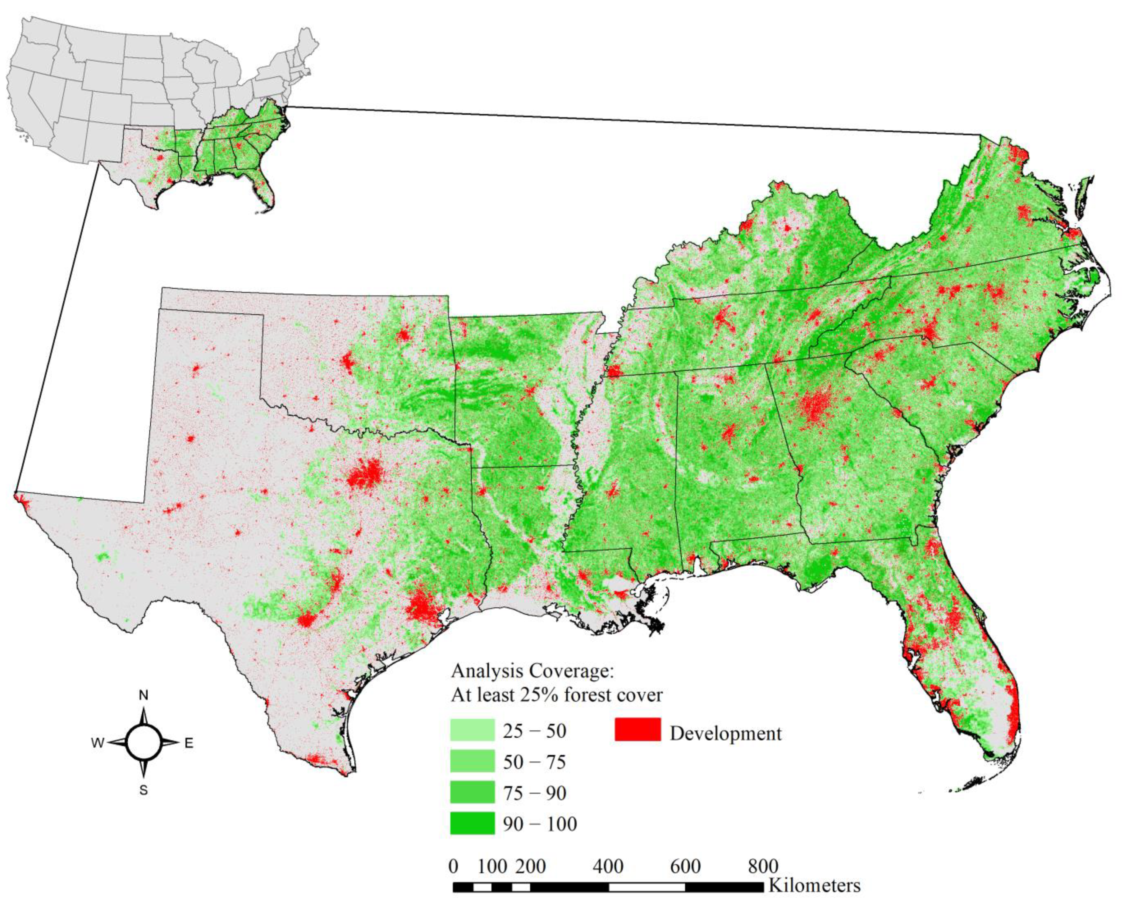
2.1. Study Region

The southern region of the administrative unit of the USDA Forest Service (USFS) is comprised of 13 US states from Virginia on the Atlantic coast, westward to Texas (Figure 1). This large region contains a wide array of biologically diverse ecosystems with varying degrees of fire dependency, including coastal pine forests and savannahs, seasonally flooded bottomland hardwood forests, montane mixed deciduous and hardwood forests, and many other forest and non-forest ecosystem types. The region is also characterized by highly fragmented land ownership with ~86% privately owned forest land and an expanding wildland–urban interface (WUI) driven by high population growth [24,25]. Reduced fire frequency through fire suppression and exclusion has been an important aspect of forest change during the past two centuries, resulting in longer fuel accumulation periods and changes in forest structure and composition [26,27]. Fuel loads can also be locally elevated by tree damage from increasingly severe weather events including coastal hurricanes. Fire regimes are today dominated by human causes, both planned and unplanned. Most wildfires in the region have human ignition sources, and prescribed fire is a widespread forest management tool, particularly in coastal plain forests [28]. Mean maximum temperatures have not risen significantly in the southern region as a whole in recent decades [29], but climate change model projections suggest that temperature and drought frequency will increase by the mid-century, potentially increasing wildfire events and reducing safe prescribed burning windows [30,31].

2.2. Expert Working Group

We used an unstructured, collaborative, co-development approach to guide all stages of the research, through a working group with weekly meetings throughout the project. The group included regional experts in wildland and prescribed fire management from relevant programs within the USFS Region 8 Regional Office (Fire & Aviation Management; Regional Information Management) and the Southeastern Region Coordinator for the National Cohesive Wildland Fire Management Strategy [4]. The core group was supplemented on an ad hoc basis by area experts from the USFS National Forest System, the Southern Group of State Foresters (https://southernforests.org/ accessed on 15 February 2023), and scientists at the USFS Southern Research Station. The working group regularly discussed data selection for the full set of spatial variables for analysis, the general approach to data synthesis and its applicability to management problems, and the credibility of spatial results.

2.3. Data Selection and Preparation

We compiled a large suite of relevant spatial variables, intended to collectively provide a description of social and ecological landscape properties that influence fire, its impacts, and its management. The expert working group assisted in identifying relevant variables and existing spatial data products. Data quality criteria for inclusion were peer-reviewed publication, public accessibility, complete spatial coverage of the study region, and recency. In selecting variables, we guarded against bias in two ways: (1) the research team and expert working group ensured that no one voice unduly drove the process and collectively provided a broad knowledge base; and (2) we erred on the side of retaining rather than eliminating variables, resulting in a large and diverse dataset. The statistical analysis (see below) then reduced redundancy and identified fundamental components of landscape variability in an objective way.

We initially identified 88 variables for inclusion from existing data products. We used program R [32] and ArcGIS software (version 10.7.1) [33] to pre-process data and then summarize variables to a grid of contiguous 1000 ha (2470 acre) hexagons covering the southern region (Figure 1). The choice of a 1000 ha landscape size for analysis was based on our intent to produce spatial results at a management-relevant scale, capable of revealing important landscape gradients at the regional level. This involved down-sampling for some spatially coarse data (e.g., gridded climate data) and up-sampling for spatially fine-grained data (e.g., land cover). Appendix A.1 provides a brief definition, source, native resolution, and method of summarization to the 1000 ha hexagon units of analysis for each variable.

We limited the analysis to hexagons with at least 25% forest cover (Figure 1), using the 2019 National Land Cover Dataset (NLCD) product to define forest cover [34]. After filtering the hexagons by forest cover, we used a Pearson Correlation matrix to examine the degree of correlation among variables [35,36]. Our statistical analysis did not require excluding moderately correlated variables (see below), but we wished to avoid duplicating essentially identical spatial information. Therefore, if any two variables had a correlation coefficient > 0.95, we retained only the one that also had lower correlation with other retained variables. This resulted in retention of 73 variables. In the following thematic sections, we overview the included data products and variables—Appendix A.1 provides the full list of 73 retained variables.

2.3.1. Fire Dynamics and History

We used modeled spatial variables from the Wildfire Risk to Communities (WRC) project [37,38] to quantify the probability of fire occurrence (burn probability) and flame length exceedance (4 feet and 8 feet), an indicator of likely burn intensity if a fire occurs. To represent mean fire return interval at the landscape scale, we used the LANDFIRE project’s Fire Return Interval variable [39]. We included data from three separate projects to quantify the history of fire in all forest lands during approximately the past two decades (year ranges for each source are given in Appendix A.1). At the scale of the hexagonal landscape units, we summarized both forest burn frequency (number of fires) and total area burned (summed across the full time period) from the USFS/NASA MODIS Burned Areas project [40] and from an archival USDA Forest Service database of reported fires [41]. We also calculated total burned area from the Monitoring Trends in Burn Severity (MTBS) program [42,43]. Each of these sources of fire records provides unique information and each has limitations. To approximate a more complete record, we used a max-composite approach to combine all three. The resulting variable used the largest burned area estimate among the three products within each landscape unit.

2.3.2. Fire and Communities

The wildland–urban interface concept uses measures of proximity and spatial mixing between natural and developed landscape components to provide information about the vulnerability of people and infrastructure to wildfire spread [24]. To quantify WUI, we summed the ‘interface’ and ‘intermix’ cover proportions from the SILVIS Lab’s WUI spatial data product [24]. We also included a WUI risk variable from the Southern Wildfire Risk Assessment project, which uses the WUI spatial pattern to index the potential wildfire risk to populations and structures [44]. We used additional variables from the WRC dataset to represent aspects of risk to infrastructure and communities—risk to potential structures, exposure type, and wildfire hazard potential [38].

We also included two variables to quantify the potential for forests to send smoke, if they burn, to populated areas at unsafe levels of exposure. Since no spatial data of this kind were available, we modeled potential smoke exposure using methods detailed in Appendix A.2. The modeling approach used a satellite-based smoke plume dataset, forest fuel load [39], and weather patterns [45] to simulate smoke plumes for all landscapes and intersected the plumes spatially with population density [37,38]. Populations were weighted for potential vulnerability to unsafe smoke exposure using a social vulnerability dataset [46] (see Section 2.3.3). The two included variables estimated potential exposure given existing fuel loads and potential exposure under a scenario of reduced fuels through forest management before wildfire occurs (Appendix A.2).

2.3.3. Social and Cultural

Firescapes are landscape types defined by unique social and ecological characteristics which, taken together, are important for understanding how fire and associated risks operate as a human–environment system. To that end, we included population and housing density from the WRC dataset as basic measures of community and infrastructure distributions [38]. To account for forest land ownership patterns we summarized the proportion of each landscape in private, federal, state, and tribal ownership [47]. We also incorporated social vulnerability measures to account for socioeconomic conditions that place communities at a disadvantage in preparing for and responding to wildfire and increase susceptibility to risks associated with wildfire [7,8,20,48]. We included spatial variables from the Socioeconomic Data and Applications Center (SEDAC) and the Centers for Disease Control (CDC) at the census tract level that quantify vulnerabilities associated with (1) economic and educational status, (2) housing type and transportation, (3) household composition and disability, (4) minority status and language, and (5) overall vulnerability [46].

2.3.4. Forest Properties

To quantify forest fuel load, a crucial measure for understanding the potential for hazardous fire, we summarized total available fuels within forested areas using the most current fuel data from the LANDFIRE program’s Fuel Characteristic Classification System [39]. We calculated the proportional cover of broad forest types (upland conifer, longleaf/slash pine, loblolly/shortleaf pine, upland hardwoods, bottomland/moist soil hardwoods) and forest stand size classes (small, medium, and large diameter trees) using spatial data modeled from the USFS Forest Inventory and Analysis (FIA) field plot data under the FIA’s BIGMAP program [49,50]. We also summarized total forest carbon stocks using BIGMAP model estimates. To estimate the risk of damage to forests from insects and disease, which can interact with other factors to influence wildfire hazard especially through tree stress and mortality, we summarized the total basal area modeled to be at risk of loss from a national USFS analysis that also relied on FIA plot data for modeling [51].

2.3.5. Landscape and Watershed Properties

We included measures of the current proportional cover of forest, agriculture, and urban development using the NLCD [34]. To quantify changes in land cover, we summarized the change in density (i.e., the proportion of pixels) of natural, agricultural, and developed cover over the past 10 and the past 20 years using the Land Change Monitoring, Assessment, and Projection (LCMAP) annual data products [52,53]. Additional landscape description included a LANDFIRE index for the departure of current vegetation conditions from reference conditions, i.e., ‘vegetation departure’ [39], and an index of decadal change in growing season greenness using the mean Normalized Difference Vegetation Index (NDVI), which is correlated with vegetation amount and productivity—this product was derived from the Landscape Dynamics Assessment Tool [54].

To quantify the importance of forest watersheds as sources of surface-derived drinking water for downstream populations, we used spatial data from the USFS Forests to Faucets 2.0 project [12] at the HUC12 watershed scale (mean size = 101.3 km²), summarized to our smaller landscape scale. We included variables for watershed importance, the size of the dependent population, natural and impervious watershed cover proportions, and the proportion of the watershed with high risk to surface drinking water from fire (wildfire hazard potential) and from land use change [12].

2.3.6. Biodiversity

Wild and prescribed fire each have important consequences for the condition of forest habitats supporting plant and wildlife species [55,56]. To represent the importance of landscapes for biodiversity conservation, we calculated the number of at-risk terrestrial species with potentially suitable habitats present, using the US Fish and Wildlife Service’s estimated current range for threatened and endangered plant and wildlife species (https://ecos.fws.gov/ accessed on 25 January 2022). We included variables for the number of wildlife species, the number of plant species, and both combined. For a broader measure of conservation value, we also summed the proportional cover of medium- to highest-priority areas from the Southeast Conservation Blueprint [57]. The Blueprint ranks lands and waters across the region where conservation activities are expected to have a significant impact based on terrestrial and aquatic ecosystem health, ecosystem services, and landscape connectivity.

2.3.7. Climate

We included variables to represent long-term climate (i.e., climatologies) during the most recent thirty years available (1992–2021). We used climate data from the statistically downscaled MACAv2 dataset, selected for use in the 2020 Resources Planning Act (RPA) Assessment and archived by the USFS [58]. This dataset includes variables summarized on a monthly timescale. We included 30-year means for five monthly variables, selected for their relevance to fire activity: mean daily minimum relative humidity in the month with the lowest value in the year, total precipitation in the month with the lowest value in the year, mean daily downward solar radiation in the month with the highest value in the year, mean daily maximum temperature in the month with the highest value in the year, and mean daily potential evapotranspiration (PET) in the month with the highest value in the year. In addition, we included the 30-year mean of the Standardized Precipitation–Evapotranspiration Index (SPEI), a standard drought index which has been correlated with wildfire occurrence and severity [59]. We calculated the SPEI from the monthly total precipitation and mean PET from the MACAv2 data, estimating drought severity on a 3-year timescale for each month (i.e., that month and the 35 preceding), relative to baseline years 1979–2008.

2.4. Statistical Analysis

We subjected the full dataset of 73 variables described above to a sequential process of factor analysis followed by cluster analysis to classify landscapes across the study region into distinctive types, which we then interpreted as firescape classes. Factor analysis uses the correlation structure among a set of variables to model a smaller number of unobserved, latent variables known as factors [60,61]. The factors quantify important dimensions of the full dataset, accounting for variation in the data with a smaller number of factors. The factors can be interpreted by examining the loadings of the original variables onto each factor, allowing for a description of the factors in terms of their ecological and social relevance.

We applied a maximum-likelihood factor analysis and rotated the factors using the varimax rotation [61]. Varimax rotation maximizes the loading of a given variable onto only one or a few factors, simplifying the interpretation of factors while maintaining orthogonality (i.e., the factors are uncorrelated with one another). Nonetheless, it is not uncommon for different components of one variable to load on different factors. To identify a sufficient number of factors to describe important dimensions of the data while keeping the number of factors manageable, we generated a scree plot of the cumulative variance explained to identify a shelf or ‘elbow’ relative to the number of factors included [62]. In choosing the final number of factors, we also took into account the interpretability of factors when different numbers were included. Maximum-likelihood-based factor analysis makes a data normality assumption, and we examined q-q plots and outliers for all variables. As expected for any large, multivariate socio-ecological dataset, we identified moderate skew for some variables but we chose to retain these considering the potential loss of information more detrimental than any mild effect of normality violations on the factor distributions [63].

We then implemented a non-hierarchical k-means cluster analysis, for which the factors were the inputs. Cluster analysis groups observations—in this case, landscapes—based on shared characteristics, maximizing within-cluster similarity and minimizing between-cluster similarity [54,64,65,66]. Cluster analysis identifies structures in multivariate data, offering advantages over similar methods in the relative ease of interpreting and communicating results [65,67]. Clusters can be thought of as categorical types into which the multidimensional data space has been partitioned and within which the input variables—in this case, the factors—exhibit characteristic value ranges. The use of orthogonal factors as inputs avoided the inclusion of multiple correlated variables in the cluster analysis [66]. Each resulting cluster (i.e., firescape class) was defined by its set of centroid values for the factors, and the firescape classes contrast with one another in terms of the underlying factors. To identify a sufficient number of clusters to describe important regional variability, we generated a scree plot of the sum of squares ratio to identify a shelf in the variance explained relative to the number of clusters included [64,68].

After assigning a firescape class membership to every 1000 ha landscape, we mapped both the firescapes and the underlying factor scores to explore their spatial patterns across the study region. We also generated a spring plot to visualize the relative similarities among firescape classes, based on Euclidean distances among the cluster centroids in the multi-dimensional factor space. Spring plotting was based on the Fruchterman–Reingold algorithm [69] implemented in the qgraph R package [70]. We conducted all other statistical analyses in program R version 4.1.2, using the base factanal and kmeans functions to perform the factor and cluster analyses, respectively [32].

3. Results

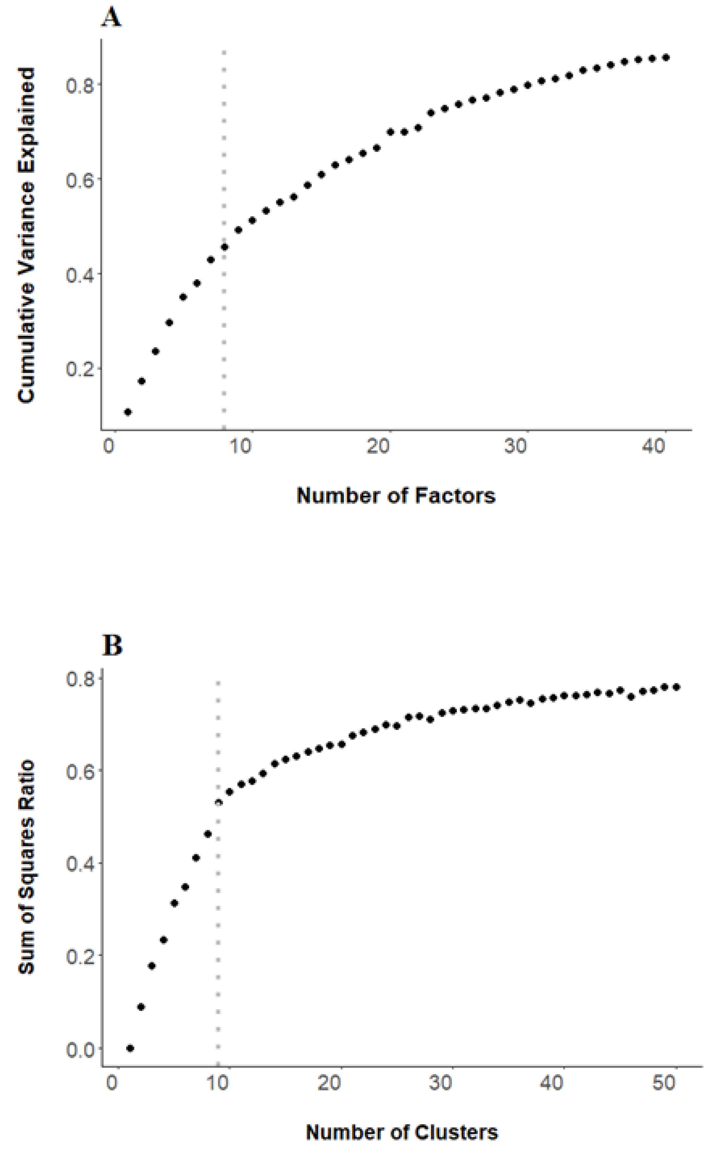
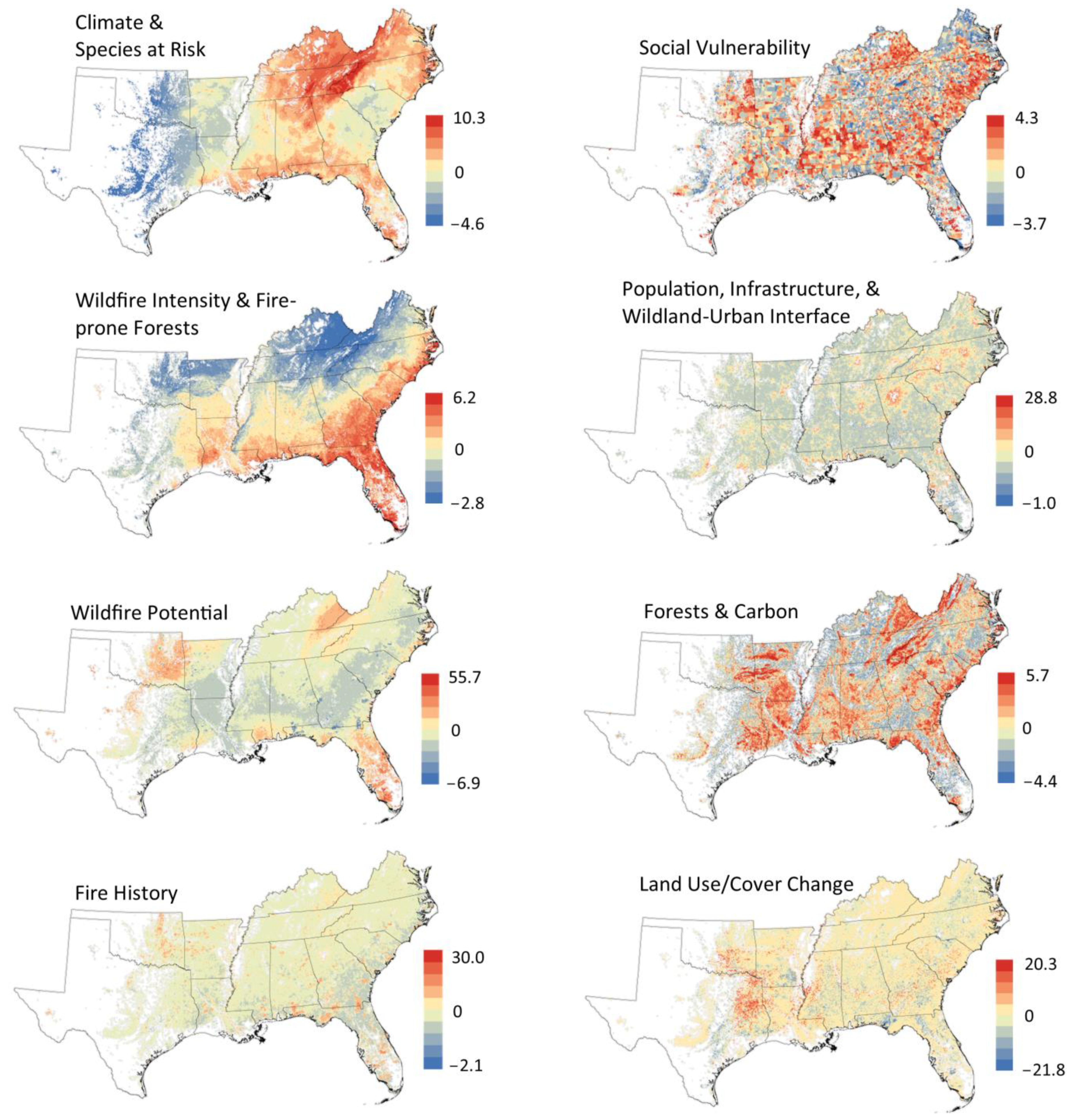
3.1. Factor Analysis

The cumulative variance explained in factor analysis with an increasing number of factors (Figure 2) resulted in a relatively smooth curve but indicated a choice of fewer than 10 factors to describe key dimensions of the data efficiently. Our final choice of eight factors was also influenced by the clear interpretability of factors with the analysis set to return eight factors (see below). All eight factors had eigenvalues greater than 1.0 and collectively explained 45.4 percent of the total variance among the 73 variables (

Table 1. Key dimensions of landscape variability important for assessing wildfire dynamics, risks, and management in southeastern US forest landscapes, identified through factor analysis of 73 spatial variables. Variance explained is the cumulative variance in the dataset accounted for by each additional factor from 1 through 8. Factor names and key characteristics were interpreted from their variable loadings (Table 2).

Factor	Var. Explained	Factor Name	Key Characteristics
1	0.076	Climate and Species at Risk	Climate (multiple variables), threatened and endangered plants and animals, large diameter forest, wildfire fuels, potential for smoke
2	0.149	Wildfire Intensity and Fire-prone Forests	Potential flame length exceedance, wildfire hazard potential, longleaf and slash pine forest, small diameter forest, hot climate
3	0.212	Fire History	Area burned and fire frequency
4	0.273	Population, Infrastructure, and Wildland–Urban Interface	Developed land use, mixed urban–forest landscapes, WUI proportion, wildfire risk in the WUI
5	0.331	Forests and Carbon	Forest cover, forest carbon stocks, conservation values, fuel load, and potential wildfire exposure
6	0.375	Wildfire Potential	Burn probability, risk to potential structures, wildfire hazard potential
7	0.416	Social Vulnerability	Multiple dimensions of socio-economic vulnerability
8	0.454	Land Use/Cover Change	Agricultural and natural land use/cover change

).

Table 2. Factor loadings of 73 spatial variables across southeastern US forest landscapes (only including variables with loadings > +/−0.30). Negative loadings indicate an inverse relationship. * Note that the WUI Risk variable expresses high risk as highly negative values. Variable descriptions are in Appendix A.1.

Factor 1: Climate and Species at Risk	Loadings	Factor 2: Wildfire Intensity and Fire-Prone Forests	Loadings	Factor 3: Fire History	Loadings	Factor 4: Population, Infrastructure, and WUI	Loadings
Min Precipitation	0.745	Longleaf/Slash Pine	0.613	Forest burn frequency, 2001–2021	0.980	Housing unit density	0.989
Min relative humidity	0.526	Proportion of watersheds with high to very high wildfire hazard potential	0.557	Forest area burned, 2001–2021	0.977	Population density	0.989
SPEI drought index	0.489	Flame length exceedance (8 ft)	0.554	Forest burn frequency, 2012–2021	0.880	Developed land cover	0.856
Stand size class: Large	0.446	Flame length exceedance (4 ft)	0.536	Maximum burned area (composite)	0.872	Proportion impervious	0.672
T and E Plants and Wildlife	0.443	Stand size class: Small	0.536	MTBS Burned area, 2000–2020	0.701	WUI Risk *	−0.651
T and E Wildlife	0.423	Max downward radiation	0.463			WUI proportion	0.350
Forest carbon stocks	0.360	Max temperature	0.436
Fuel Load	0.336	Loblolly/Shortleaf Pine	0.409
Potential wildfire smoke exposure	0.328	Bottomland/Moist Soil Hardwoods	0.378
Downstream drinking water population	0.312	Wildfire hazard potential	0.344
Potential evapotranspiration	−0.949	Vulnerability index: Minority status and language	0.343
Max temperature	−0.765	Natural-caused fires, 2000–2018	0.330
Max downward radiation	−0.713	Upland Hardwoods	−0.819
Stand size class: Medium	−0.470	Downstream drinking water population	−0.719
Upland Conifer	−0.438	Watershed importance for surface drinking water	−0.623
Non-stocked forest type group	−0.344	Stand size class: Large	−0.407
Non-stocked size class	−0.337	SPEI drought index	−0.328
Vulnerability index: Minority status and language	−0.300
Factor 5: Forests and Carbon	Loadings	Factor 6: Wildfire Potential	Loadings	Factor 7: Social Vulnerability	Loadings	Factor 8: Land Use/Cover Change	Loadings
Forest land cover	0.887	Risk to potential structures	0.945	Vulnerability index: Overall	0.967	Natural cover density change, 2010 to 2019	0.980
Forest carbon stocks	0.817	Burn probability	0.937	Vulnerability index: Socioeconomic	0.811	Natural cover density change, 2000 to 2019	0.792
Proportion natural cover	0.654	Wildfire hazard	0.718	Vulnerability index: Housing type and transportation	0.755	Agriculture cover density change 2010 to 2019	−0.951
Fuel Load	0.546	T and E Wildlife	0.341	Vulnerability index: Household composition and disability	0.604
Projected total basal area loss from all pests	0.518	T and E Plants and Wildlife	0.314	Vulnerability index: Minority status and language	0.428
Conservation priority areas	0.453
Exposure type	0.391
Agricultural land cover	−0.802
Wildland–Urban Interface (WUI)	−0.302

shows variable loadings on each factor, excluding factor loadings ˂ +/−0.30 (Appendix A.3 provides the complete factor loading results). Each factor showed unique geographic variation across the study region (Figure 3—note that factor scores are standardized and have a mean value of zero).

We interpreted key characteristics of the factors and gave them descriptive names (Table 1) based on their variable loadings (Table 2). Here we provide additional detail for the individual factors. We named Factor 1 Climate and Species at Risk. Eighteen variables had loadings >0.30 for this factor, and the six with the highest loadings were all climate variables. Landscapes with high values were characterized by cool, wet climate conditions with low drought potential. High values for this factor were also associated with forest in the large diameter class, presence of threatened and endangered species habitats, high fuel load and forest carbon stocks, potential to send hazardous levels of wildfire smoke to populated areas, and low cover of upland conifer forest. Landscapes with the highest values were mainly in the interior highlands, especially the southern Appalachian Mountains, and to a lesser extent along the coastal plains (Figure 3).

Factors 2, 3, and 6 quantified various aspects of fire behavior and related forest ecological properties. We named Factor 2 Wildfire Intensity and Fire-prone Forests. There were 17 variables with loadings >0.30 for this factor. Landscapes with high values were primarily characterized by high cover of pine forest types and low cover of upland hardwood forest, high wildfire hazard potential, and high wildfire flame length exceedance probabilities. There were additional positive associations with forest in the small diameter class and hot climate, both of which can contribute to wildfire hazard. There were negative associations of this factor with watershed importance for surface drinking water and the size of the downstream drinking water population. Places with the highest values were widespread along the Gulf and Atlantic coastal plains and in Florida. We named Factor 3 Fire History, with five variables having loadings >0.30. This factor principally characterized the fire history of landscapes—high values were associated with both the frequency of fire occurrence and the total area burned over the past two decades. Landscapes with very high values were relatively uncommon and widely dispersed (Figure 3). We named Factor 6 Wildfire Potential. Five variables had loadings >0.30 for this factor. Landscapes with high values were characterized by high burn probability, high risk to potential structures, and high wildfire hazard potential. This factor also had moderate positive loadings for threatened and endangered species habitats, reflected by landscapes with the highest values concentrated in the Florida peninsula. Factors 2 and 6 were related but not equivalent. They sorted variables into those associated with burn intensity and those associated with burn probability, respectively. These are two principal aspects of wildfire hazard—the likelihood of fire occurrence and the likely intensity of fire if it occurs.

Factors 4 and 7 quantified social and socioecological landscape properties. We named Factor 4 Population, Infrastructure, and Wildland–Urban Interface. Five variables had loadings >0.30 for this factor, characterizing housing and population density and the proportion of developed land and impervious surface. Landscapes with high values were also characterized by high WUI proportion and high WUI risk and were spatially clustered near towns and cities (Figure 3). We named Factor 7 Social Vulnerability. All five social vulnerability variables in the full dataset had loadings >0.30 for this factor, and these were the only variables with loadings >0.30. All loadings were positive, indicating that landscapes with high values were characterized by high social vulnerabilities in terms of socio-economic status; household composition and disability; minority status and language spoken in the household; and housing and transportation types. Landscapes with high values were distributed in a broad arc across the Atlantic and Gulf coastal plains and lower Piedmont subregions and in some interior highland areas including eastern Kentucky and eastern Oklahoma (Figure 3).

Finally, factors 5 and 8 quantified important forest characteristics and aspects of land cover. We named factor 5 Forests and Carbon. Nine variables had loadings >0.30 for this factor. High values were associated with high proportions of forest cover and natural cover, low proportions of agricultural cover and WUI, and high forest carbon stocks, forest fuel load, forest at risk from insects and disease, and high-priority conservation areas. Landscapes with high values were concentrated in places with extensive forest cover throughout the region. We named factor 8 Land Use/Cover Change. Three variables had loadings >0.30 for this factor, all quantifying change in the proportion of natural or agricultural land. Landscapes with high values were characterized by increasing natural land cover and decreasing agricultural cover—mainly reflecting conversion from agriculture to a variety of land uses in the generalized ‘natural’ cover class [71,72]. Landscapes with positive values were widespread and most frequently in the western part of the region (e.g., east Texas) and along the Atlantic coastal plain. Areas with negative values, indicating natural cover loss, were also widespread, but interior highland landscapes mostly showed values near zero for this factor.

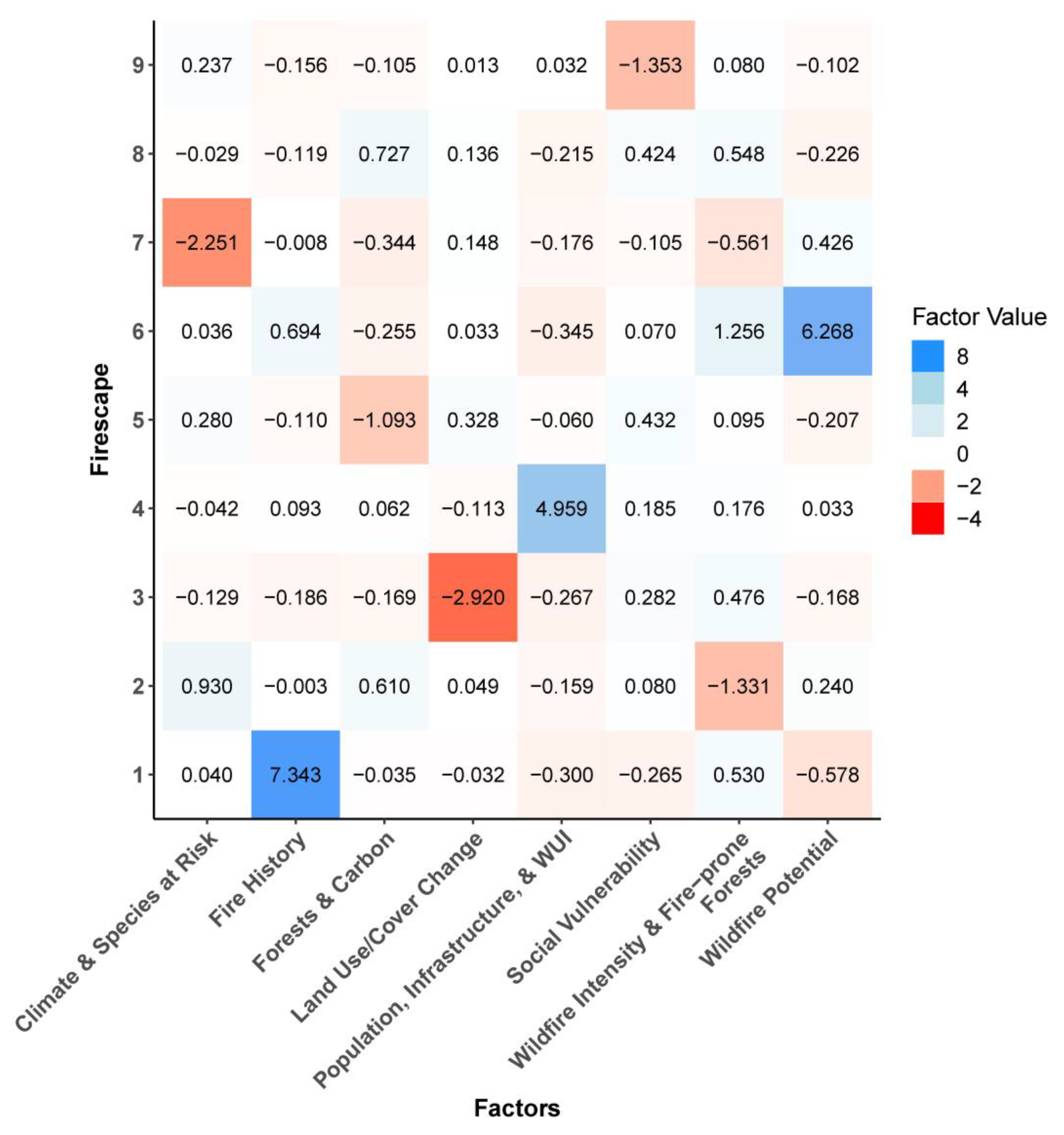
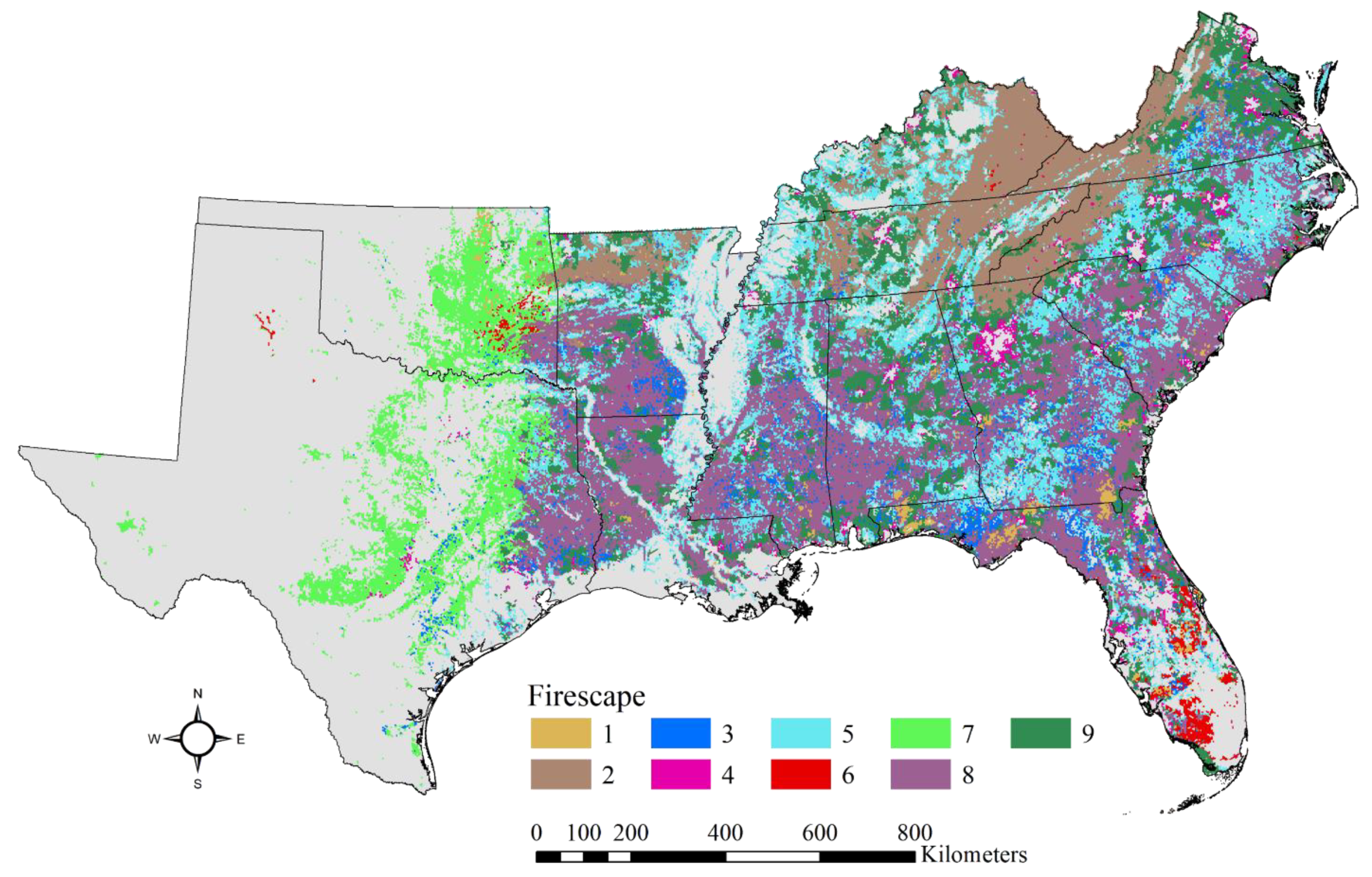
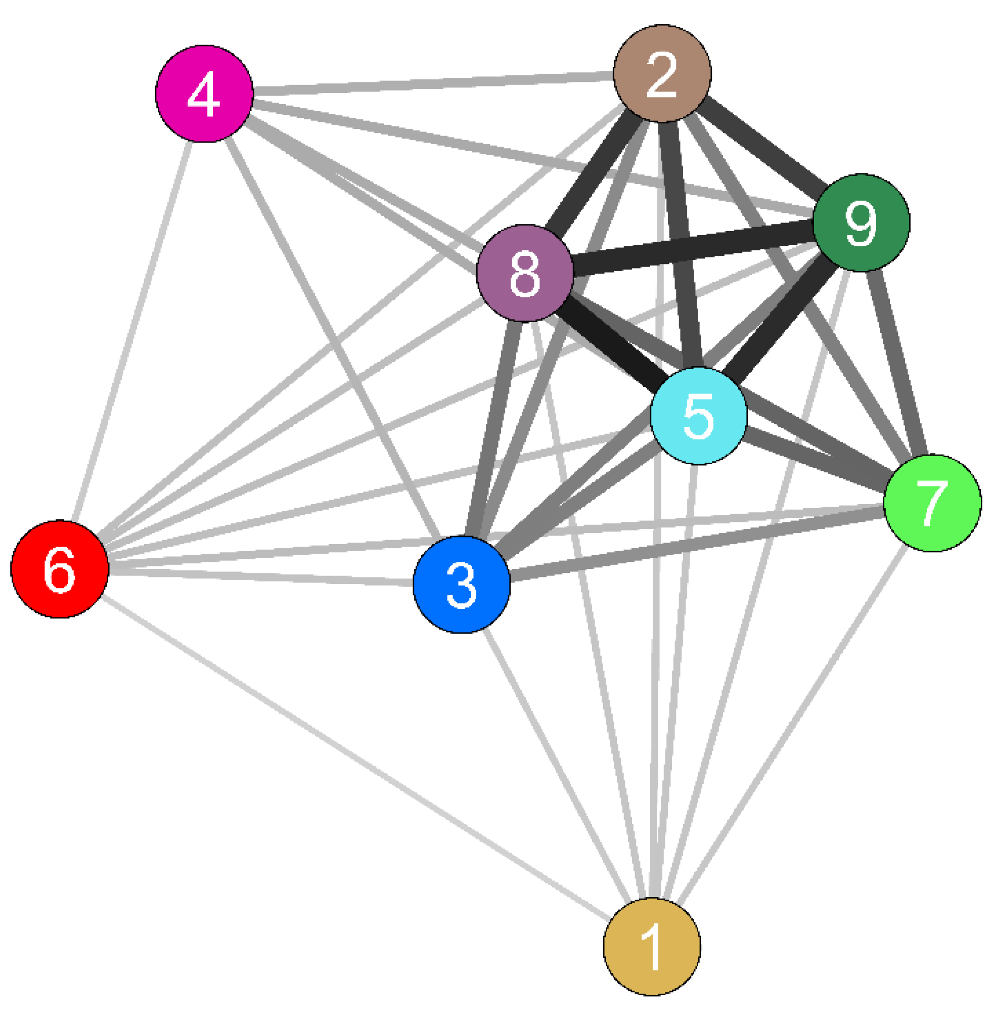
3.2. Cluster Analysis

Scree plotting indicated a choice of nine (9) clusters to efficiently partition the eight-factor data space (Figure 2B). The resulting clusters, interpreted as firescape classes, were defined by their centroid values for all eight factors (Figure 4). We developed plain-language names and descriptions of the classes based on these characteristic factor values and the distinctive geographic pattern of each class across the study region (

Table 3. Firescape classification of southeastern US lands with at least 25% forest cover, generated through factor and cluster analysis of 73 spatial variables. Narrative descriptions are based on interpretation of the factor values characteristic of each class (Figure 4).

Cluster	Firescape Name	Key Characteristics	Area (km2)
1	History of wildfire, potential for intense fire	Rural areas with recent history of fire, pine forest cover, moderate potential for high intensity fire, low burn probability, low risk to structures, low population density, low social vulnerability	15,220
2	Cool and wet broadleaf mountain forests	Mountain forest landscapes with cool, wet climate, high deciduous (non-conifer) forest cover, high conservation value, high fuel load and carbon stocks, moderate risk from wildfire smoke, low potential for intense fire	182,930
3	Rural pine forest, conversion to agricultural lands	Moderate pine forest cover, natural land cover conversion to agriculture, moderate potential for high-intensity fire, low population density and wildland–urban interface, moderate social vulnerability	58,880
4	Urban periphery landscapes	Exurban and urbanizing landscapes with high population density, development, WUI, and WUI risk	33,940
5	Rural agriculture, vulnerable communities, and low wildfire potential	Rural areas with low forest cover, carbon stocks and fuel load, mild climate, low burn probability, low risk to structures and wildfire hazard potential, high social vulnerability, moderate gain of natural land cover	284,140
6	Rural mixed forest with hazardous fire potential	High potential for hazardous fire, history of wildfire, low/mixed forest cover with some pine and hardwoods, low population density and WUI	14,080
7	Warm and dry, mixed woodlands	Warm and dry climate, low to moderate forest cover with mixed hardwoods and conifers, low carbon stocks, wildfire potential but low potential for intense fire	126,250
8	Rural pine forests, intense fire, and vulnerable communities	High pine forest cover, fuel load, and carbon stocks, potential for intense fire, low population density, high social vulnerability	382,690
9	Semi-rural with low social vulnerability and moderate climate	Low social vulnerability, moderate forest cover, moderate climate, low–moderate wildfire potential and fire history	226,080

, Figure 5). Their geographic distributions (Figure 5) were associated in part with well-known biophysical variation in the region, including coastal plain, Piedmont, and mountain subregions, and with regional variations in forest types, fire histories, aspects of the built environment (e.g., urban development), human geography (e.g., varying social vulnerabilities), and climate. Spring plotting of cluster centroids revealed relative similarities and differences among the firescape classes (Figure 6). For example, classes 2, 5, 8, and 9 formed a closely related group, with wider distances among the remaining classes. Classes 2, 5, 8, and 9 also had the largest landscape memberships among all classes, collectively occupying the strong majority of the forest land area in the region (Table 3).

3.3. Firescape Descriptions

Firescape 1 (History of wildfire, potential for intense fire) was characterized by a very high centroid value for the Fire History factor, a moderately high centroid value for the Wildfire Intensity and Fire-prone Forests factor, and low values for the Population, Infrastructure, and WUI, Wildfire Potential, and Social Vulnerability factors. These attributes suggest rural landscapes with recent fire history, pine forest, and moderately lower social vulnerabilities than most other firescape classes. Isolated landscapes across the region were included in this firescape class, with larger concentrations in northern Florida and southern Georgia—its distribution in the northern part of the region was extremely limited.

Firescape 2 (Cool and wet broadleaf mountain forests) had high centroid values for the Climate and Species at Risk and Forests and Carbon factors, and a moderately high value for the Wildfire Potential factor. It had low centroid values for the Potential Wildfire Intensity and Fire-prone Forests and Population, Infrastructure, and WUI factors. These attributes suggest rural landscapes with cool, moist climates, dominated by a high cover of mostly non-conifer, upland hardwood forest. Although moderate potential for wildfire was suggested, a low likelihood of high-intensity fire was also suggested. Landscapes in this firescape class were common but limited to the northern parts of the region within interior highland subregions including the southern Appalachian Mountains, Cumberland Plateau, and Ozark Mountains.

Firescape 3 (Rural pine forest, conversion to agricultural lands) was characterized by a strongly negative centroid value for the Land use/cover change factor, indicating gain of agricultural cover and loss of natural cover. This firescape also had an above-average centroid value for the Wildfire Intensity and Fire-prone Forests factor, below average value for the Population, Infrastructure, and WUI factor, and an above average value for the Social Vulnerability factor. These attributes suggest rural lands with moderate social vulnerability, pine forests with moderate potential for high-intensity fire, and a recent history of land conversion to agriculture.

Firescape 4 (Urban periphery landscapes) was mainly characterized by a very high centroid value for the Population, Infrastructure, and WUI factor. This firescape was concentrated in the periphery of urban and developed areas across the region, where population density is high but landscapes also have some forest cover.

Firescape 5 (Rural agriculture, vulnerable communities, and low wildfire potential) had a strongly negative centroid value for the Forests and Carbon factor, above average values for the Social Vulnerability, Climate and Species at Risk, and Land Use/Cover Change factors, and a below average value for the Wildfire Potential factor. These attributes suggest agricultural landscapes with low forest cover (although all landscapes included in analysis had at least 25% forest cover), high social vulnerability, low wildfire probability, mild climate, and some conversion to natural land cover. This was a common firescape class distributed throughout the region but mostly concentrated in the east and north, with the notable exception of a large agricultural region in southern Georgia.

Firescape 6 (Rural mixed forest with hazardous fire potential) had very high centroid values for the Wildfire Potential and Wildfire Intensity and Fire-prone Forests factors and an above average value for the Fire History factor. Together with below average values for the Population, Infrastructure, and WUI and Forests and Carbon factors, these attributes suggest rural landscapes with mixed non-forest, pine, and hardwood forest covers, strongly characterized by potential for intense fire and a recent history of fire. This class was common in southern Florida and had some occurrence in eastern Oklahoma, but was rare elsewhere.

Firescape 7 (Warm and dry, mixed woodlands) had a very low centroid value for the Climate and Species at Risk factor, indicating hot and dry long-term climate conditions. Low centroid values for the Forests and Carbon and Wildfire Intensity and Fire-prone Forests factors, and an above average value for the Wildfire Potential factor, suggest mixed landscapes with low hardwood and conifer forest cover and high wildfire potential but low potential for high-intensity fire. This firescape class was restricted to east-central Texas and eastern Oklahoma and was dominant in that westernmost part of the study region.

Firescape 8 (Rural pine forests, intense fire and vulnerable communities) had high centroid values for the Forests and Carbon and Wildfire Intensity and Fire-prone Forests factors, moderately low values for the Wildfire Potential and Population, Infrastructure, and WUI factors, and an above average value for the Social Vulnerability factor. These attributes indicate high forest cover dominated by pine forest types with potential for high-intensity fire in rural landscapes with high social vulnerabilities. This firescape was common and widespread, accounting for the most rural forest lands in the coastal plain and Piedmont subregions, as well as pine forest lands west of the Mississippi River.

Firescape 9 (Semi-rural with low social vulnerability and moderate climate) had the lowest centroid value of any firescape class for the Social Vulnerability factor, an above average value for the Climate and Species at Risk factor, and moderately low values for the Forests and Carbon, Wildfire Potential, and Fire History factors. It also had a centroid value near zero (average) for the Population, Infrastructure, and WUI factor. Taken together, these attributes indicate semi-rural landscapes with unusually low social vulnerability, moderate forest cover and climate, and low fire activity. This firescape class was widespread but more common in the northern and central parts of the region, with concentrations in semi-rural areas broadly surrounding towns and cities.

4. Discussion

The sequential application of factor and cluster analyses to a large, carefully chosen set of spatial variables constitutes a data-driven way to identify and map landscape types that can be characterized as firescapes. The results of this analysis can provide decision support to forest managers, planners, and other stakeholders in the study region by helping to inform locally appropriate management strategies and investments aimed at reducing risks associated with wildfire, building community and forest resilience to fire, and improving conservation outcomes. Management tools for such efforts include but are not limited to prescribed fire, mechanical fuel treatments, hardening homes against fire, educational outreach, community capacity building, and other forms of community engagement.

4.1. Socio-Ecological Implications

Our results translate a large number of social and ecological landscape properties into synthetic information that can support the evaluation of needs and opportunities concerning wild and prescribed fire management. Here, we illustrate this with examples that relate firescape attributes to management priorities, without reviewing each firescape class exhaustively.

The Social Vulnerability factor and the social vulnerability attributes of the different firescape classes provide geographic information about the co-occurrence of vulnerable populations and potential for hazardous fire, based on variables representing income, education, age, disability, minority status, housing type, and transportation. Recent research suggests that economically stressed, historically disadvantaged, and underserved populations experience greater vulnerability to wildfires compared to other communities [7,8,20,48]. Examining the intersection between social vulnerability and wildfire risk is therefore imperative. Our results suggest that this intersection is most pronounced in landscapes such as those included in firescapes 8 (Rural pine forest, intense fire, and vulnerable communities) and 3 (Rural pine forest and conversion to agriculture), where high social vulnerability and potential for high-intensity fire coincide. The Rural pine forest, intense fire, and vulnerable communities firescape in particular spans the coastal plain from eastern Texas to eastern North Carolina and Virginia, a region with strong existing investments in frequent prescribed fire [28,73]. Dominant ecological and biophysical characteristics of this firescape—heavy forest cover primarily in pine forest types, high cover of small-diameter forest stands, high flame length exceedance probabilities and wildfire hazard potential, and warm climate—all indicate an ongoing need to reduce hazardous fuels.

However, social characteristics of this firescape include mostly rural communities with moderate or high social vulnerability. In such places, while traditional fuel reduction measures including prescribed fire remain important, increased attention to the heightened vulnerability of communities to smoke from prescribed fire is also warranted [20]. Safe risk management near communities may be advanced through a combination of treatments, such as mechanical thinning prior to prescribed fire [74,75]. Education, outreach, and other investments to enhance community preparedness for both prescribed fire and wildfire can play an outsized role in improving outcomes in these places [3,7].

Prescribed fire can be even more challenging in landscapes with dense human populations and infrastructure, where wildfire risks may still be high but a mixture of management approaches may be more suitable. Firescape 4 (Urban Periphery Landscapes) exemplifies this situation, characterized mainly by high values for the Population, Infrastructure, and WUI factor. The co-occurrence of forest cover with urban development in this firescape, and in WUI landscapes more generally, clearly carries wildfire risk management concerns. But social perceptions around prescribed fire, and risks of escaped fire and smoke exposure, call for careful planning with affected communities, potentially taking advantage of alternatives such as mechanical fuel reductions or specialized site preparation prior to prescribed fire.

Other attributes of the firescapes and factors suggest opportunities for improving forest conservation outcomes while also reducing risks for surrounding communities. The factors Forests and Carbon and Climate and Species at Risk provide geographic information about conservation priorities including maintaining a suitable habitat for threatened and endangered species, maintaining forest carbon storage capacity and watershed quality, and reducing risks to forest trees from insects and disease. Prescribed fire can play a role in advancing each of these goals [10,76,77,78]. The firescape Cool and Wet Broadleaf Mountain Forests, restricted to interior highlands subregions, had high values for both of those factors, suggesting high conservation value in terms of these goals. This firescape is also characterized by a cool, wet climate and low potential for high-intensity fire, combined with moderate wildfire potential, high fuel loads, and potential to send smoke at unsafe levels to vulnerable populations. Taken together, these results suggest that landscapes in this firescape class could benefit in multiple ways from increased investments in prescribed fire. Fuel reduction via prescribed fire can help reduce the risk of exposing nearby communities—and more distant urban areas beyond the extent of the firescape—to uncontrolled emissions of harmful smoke from wildfires under high-fuels conditions [79,80]. Biodiversity values can be advanced through the direct ecological benefits of prescribed fire [55,56,77], and ecosystem services potentially compromised by wildfire, including forest carbon storage, drinking water quality, and sustainable forestry, can also see long-term benefits from prescribed fire programs [10,81].

4.2. Quantitative Firescapes: Advantages and Applications

The quantitative clustering approach we present allows the classification and delineation of firescapes to be largely determined by the data. This can help avoid undue reliance on preconceived notions of important landscape patterns for determining how and where firescapes should be delineated. A challenge with the data-driven approach is the potential sensitivity of the analysis to data quality and the selection of data inputs. We sought to include a wide variety of relevant social and ecological landscape properties to produce broadly applicable firescape delineations and to avoid over-determining or biasing the results with only a few influential variables or factors. The use of expert elicitation proved crucial for robust data discovery, selection, and—in the case of smoke exposure potential—identifying the need for new data. Regardless, the information that the firescapes provide is limited to what can be derived from the input data, and their interpretation should take this into account.

An important rationale for our use of factor analysis was that many of the variables used to describe landscape properties, which can initially appear unrelated, in fact may be shaped by shared underlying drivers and may therefore be correlated. Factor analysis simplifies the cluster analysis by first reducing the environmental space to these shared, and in a sense more fundamental, dimensions [54]. This makes interpretation of the firescapes more straightforward while still retaining the most important dimensions of variability in the data. The Climate and Species at Risk factor illustrates this well, with high loadings for more variables than any other factor. Positive values for this factor were associated with a cool and moist climate, presence of at-risk species habitats, extensive forest cover, upland deciduous and mixed forests, high fuel load, and large-diameter forest stands. All of these properties are indicative of forest landscapes in and around the Appalachian Mountains and Cumberland Plateau (Figure 3), where basic climatic, physiographic, and land use patterns have tended to shape a variety of landscape properties. The factors and their maps quantify shared patterns such as these, facilitating a more general understanding.

A benefit of our data-driven approach is that it can be applied at finer or coarser spatial scales, or even hierarchically, depending on data availability and the intended purposes of a firescape analysis (e.g., for more local or national landscape description). We chose a fairly fine spatial scale of analysis and arbitrary hexagonal units to allow gradients in the data to determine firescape delineations while de-emphasizing overly precise or pre-determined local boundaries. But a similar analysis could be performed using spatial units such as HUC watersheds, which are commonly used for planning and decision making [82], or firesheds, which have been used in wildfire risk analysis in the western US [83].

We did not include parameters for spatial location or adjacency in the cluster analysis, treating individual landscape units as though they were spatially independent. The clear spatial contiguity of landscapes in a given firescape (Figure 5) resulted instead from autocorrelation in the input data describing landscape properties—a typical characteristic of spatial data. Although a spatial clustering routine could be applied if stronger contiguity of firescapes were desired, advantages of not doing so are twofold. First, a preference for spatial proximity can force landscapes into a class other than what would be assigned if only the social and ecological properties of principal concern are considered. Second, when spatial proximity is not a parameter, landscapes with similar properties but separated by large distances can easily fall within the same firescape class. This is clear in our spatial results, with disjunct pockets of a given firescape occurring across the region. For example, firescape 6 (Rural mixed forest with hazardous fire potential) had two widely separated centers of abundance, in Florida and Oklahoma, and even within each of those areas the distribution of this firescape was fragmented. This example also illustrates that landscapes as clearly dissimilar as those in eastern Oklahoma and central Florida can nonetheless share properties that are important for determining how fire operates, and affects people, in those places.

Finally, quantitative firescapes may be expected to change over time as the landscape properties that determine firescape membership change. Population densities, community demographics, climate, fuel load, WUI, and other landscape properties in the analysis all may change over time. To the extent that these changes are monitored, changes in the distribution of firescapes can be assessed through re-analysis of the updated data. This also provides a quantitative means of assessing possible future change, using modeled data under a variety of future scenarios. In particular, given that climate change projections indicate conditions favoring increased wildfire activity [1,2], assessing plausible future change in firescape distributions has relevance in various planning and decision-making contexts.

5. Summary

Firescape types carry distinctive implications for wildfire, ecosystem management tools such as prescribed fire, and their consequences for people and resources [22]. They integrate biophysical and social descriptions to characterize landscapes in terms of the physical and cultural systems that affect fire and are affected by fire. As a result, they have relevance for issues that are seeing renewed emphasis in response to the ongoing wildfire crisis, including but not limited to social vulnerabilities and inequities with respect to wildfire impacts, ecosystem services placed at risk such as forest carbon storage and clean water provisioning, and the role of expanded prescribed fire efforts in mitigating risks. Firescapes provide a broad-scale context for developing fire management strategies appropriate to prevailing landscape conditions. Given ongoing and expected future social, ecological, and climate change, the distribution of firescape types may also be expected to change, highlighting their potential as a tool for dynamic landscape monitoring and projection.

The spatial data products provided by the firescapes analysis have a variety of potential research applications, in addition to their management applications. For example, quantitative firescapes provide relevant information for understanding risks associated with wildfire, but our analysis does not in itself constitute a formal risk assessment. Elsewhere, we report a quantitative risk assessment based on Bayesian network modeling, using the factors generated in our firescapes analysis as model inputs [84]. The risk analysis quantifies spatial gradients in risks to people and ecosystem services from wildfire and uses a scenario-based approach to quantify the capacity of fuel reduction decisions to reduce risk. The firescapes analysis and the risk analysis provide distinct and complementary information for risk management, including, but not limited, to prescribed fire planning. The risk assessment reported by [1,2] relies strongly on the data reduction and identification of key dimensions of landscape variability provided by the firescapes analysis. We suggest that there are likely additional research applications not yet pursued or conceived that could also benefit.

References

1. Greenberg, C.H.; Collins, B. Fire Ecology and Management: Past, Present, and Future of US Forested Ecosystems; Springer: Cham, Switzerland, 2021. [Google Scholar]
2. Vose, R.; Easterling, D.R.; Kunkel, K.; LeGrande, A.; Wehner, M. Temperature changes in the United States. In Climate Science Special Report: Fourth National Climate Assessment; U.S. Global Change Research Program: Washington, DC, USA, 2017; Volume 1. [Google Scholar]
3. Moritz, M.A.; Hazard, R.; Johnston, K.; Mayes, M.; Mowery, M.; Oran, K.; Parkinson, A.M.; Schmidt, D.A.; Wesolowski, G. Beyond a Focus on Fuel Reduction in the WUI: The Need for Regional Wildfire Mitigation to Address Multiple Risks. Front. Glob. Chang. 2022, 5, 848254. [Google Scholar] [CrossRef]
4. Wildland Fire Leadership Council. The National Strategy: The Final Phase in the Development of the National Cohesive Wildland Fire Management Strategy; United States Department of Agriculture and United States Department of the Interior: Washington, DC, USA, 2014; pp. 1–93. [Google Scholar]
5. National Interagency Coordination Center. National Interagency Coordination Center Wildland Fire Summary and Statistics Annual Report 2022. Available online: https://www.nifc.gov/sites/default/files/NICC/2-Predictive%20Services/Intelligence/Annual%20Reports/2022/annual_report.2.pdf?mf_ct_campaign=msn-feed&utm_content=syndication (accessed on 1 May 2023).
6. Reid, C.E.; Brauer, M.; Johnston, F.H.; Jerrett, M.; Balmes, J.R.; Elliott, C.T. Critical Review of Health Impacts of Wildfire Smoke Exposure. Environ. Health Perspect. 2016, 124, 1334–1343. [Google Scholar] [CrossRef] [PubMed]
7. Davies, I.P.; Haugo, R.D.; Robertson, J.C.; Levin, P.S. The unequal vulnerability of communities of color to wildfire. PLoS ONE 2018, 13, e0205825. [Google Scholar] [CrossRef] [PubMed]
8. Palaiologou, P.; Ager, A.A.; Nielsen-Pincus, M.; Evers, C.R.; Day, M.A. Social vulnerability to large wildfires in the western USA. Landsc. Urban Plan. 2019, 189, 99–116. [Google Scholar] [CrossRef]
9. Liu, Y.; Prestemon, J.P.; Goodrick, S.L.; Holmes, T.P.; Stanturf, J.A.; Vose, J.M.; Sun, G. Future Wildfire Trends, Impacts, and Mitigation Options in the Southern United States. In Climate Change Adaptation and Mitigation Management Options: A Guide for Natural Resource Managers in Southern Forest Ecosystems; Vose, J.M., Klepzig, K.D., Eds.; CRC Press–Taylor and Francis: Boca Raton, FL, USA, 2014; pp. 85–126. [Google Scholar]
10. Caldwell, P.V.; Elliott, K.J.; Liu, N.; Vose, J.M.; Zietlow, D.R.; Knoepp, J.D. Watershed-scale vegetation, water quantity, and water quality responses to wildfire in the southern Appalachian mountain region, United States. Hydrol. Process. 2020, 34, 5188–5209. [Google Scholar] [CrossRef]
11. Lockaby, G.; Nagy, C.; Vose, J.M.; Ford, C.R.; Sun, G.; McNulty, S.; Caldwell, P.; Cohen, E.; Moore Myers, J. Forests and Water. In The Southern Forest Futures Project: Technical Report; General Technical Report SRS-178; Wear, D.N., Greis, J.G., Eds.; US Department of Agriculture Forest Service, Southern Research Station: Asheville, NC, USA, 2013; pp. 309–339. [Google Scholar]
12. Mack, E.; Lilja, R.; Claggett, S.; Sun, G.; Caldwell, P. Forests to Faucets 2.0: Connecting Forests, Water, and Communities; GTR-WO-99; United States Department of Agriculture Forest Service: Washington, DC, USA, 2022. [Google Scholar]
13. Essen, M.; McCaffrey, S.; Abrams, J.; Paveglio, T. Improving wildfire management outcomes: Shifting the paradigm of wildfire from simple to complex risk. J. Environ. Plan. Manag. 2023, 66, 909–927. [Google Scholar] [CrossRef]
14. Ott, J.E.; Kilkenny, F.F.; Jain, T.B. Fuel treatment effectiveness at the landscape scale: A systematic review of simulation studies comparing treatment scenarios in North America. Fire Ecol. 2023, 19, 10. [Google Scholar] [CrossRef]
15. Urza, A.K.; Hanberry, B.B.; Jain, T.B. Landscape-scale fuel treatment effectiveness: Lessons learned from wildland fire case studies in forests of the western United States and Great Lakes region. Fire Ecol. 2023, 19, 1. [Google Scholar] [CrossRef]
16. Kobziar, L.N.; Godwin, D.; Taylor, L.; Watts, A.C. Perspectives on trends, effectiveness, and impediments to prescribed burning in the southern US. Forests 2015, 6, 561–580. [Google Scholar] [CrossRef]
17. Kolden, C.A. We’re not doing enough prescribed fire in the Western United States to mitigate wildfire risk. Fire 2019, 2, 30. [Google Scholar] [CrossRef]
18. Stanturf, J.A.; Goodrick, S.L. Fire. In The Southern Forest Futures Project; General Technical Report SRS-GTR-178; Wear, D.N., Greis, J.G., Eds.; U.S. Department of Agriculture, Forest Service, Southern Research Station: Asheville, NC, USA, 2013; pp. 509–542. [Google Scholar] [CrossRef]
19. Naeher, L.P.; Achtemeier, G.L.; Glitzenstein, J.S.; Streng, D.R.; Macintosh, D. Real-time and time-integrated PM2. 5 and CO from prescribed burns in chipped and non-chipped plots: Firefighter and community exposure and health implications. J. Expo. Sci. Environ. Epidemiol. 2006, 16, 351–361. [Google Scholar] [PubMed]
20. Gaither, C.; Goodrick, S.; Murphy, B.; Poudyal, N. An Exploratory Spatial Analysis of Social Vulnerability and Smoke Plume Dispersion in the U. S. South. Forests 2015, 6, 1397–1421. [Google Scholar] [CrossRef]
21. US Environmental Protection Agency. Comparative Assessment of the Impacts of Prescribed Fire Versus Wildfire (CAIF): A Case Study in the Western U.S.; EPA/600/R-21/197; Center for Public Health & Environmental Assessment: Research Triangle Park, NC, USA, 2021; p. 438.
22. Smith, A.M.S.; Kolden, C.A.; Paveglio, T.B.; Cochrane, M.A.; Bowman, D.M.; Moritz, M.A.; Kliskey, A.D.; Alessa, L.; Hudak, A.T.; Hoffman, C.M.; et al. The Science of Firescapes: Achieving Fire-Resilient Communities. Bioscience 2016, 66, 130–146. [Google Scholar] [CrossRef] [PubMed]
23. Crawford, B.A.; Katz, R.A.; McKay, S.K. Engaging Stakeholders in Natural Resource Decision-Making; Environmental Laboratory, Engineer Research and Development Center: Vicksburg, MI, USA, 2017; pp. 1–15. [Google Scholar]
24. Radeloff, V.C.; Helmers, D.P.; Kramer, H.A.; Mockrin, M.H.; Alexandre, P.M.; Bar-Massada, A.; Butsic, V.; Hawbaker, T.J.; Martinuzzi, S.; Syphard, A.D.; et al. Rapid growth of the US wildland-urban interface raises wildfire risk. Proc. Natl. Acad. Sci. USA 2018, 115, 3314–3319. [Google Scholar] [CrossRef] [PubMed]
25. Butler, B.J.; Wear, D.N. Forest ownership dynamics of southern forests. In The Southern Forest Futures Project: Technical Report; US Department of Agriculture Forest Service, Southern Research Station: Asheville, NC, USA, 2013; pp. 1–552. [Google Scholar]
26. Landers, J.L.; Van Lear, D.H.; Boyer, W.D. The longleaf pine forests of the southeast: Requiem or renaissance? J. For. 1995, 93, 39–44. [Google Scholar]
27. Vose, J.M.; Peterson, D.L.; Fettig, C.J.; Halofsky, J.E.; Hiers, J.K.; Keane, R.E.; Loehman, R.; Stambaugh, M.C. Fire and Forests in the 21st Century: Managing Resilience Under Changing Climates and Fire Regimes in USA Forests. In Fire Ecology and Management: Past, Present, and Future of US Forested Ecosystems; Greenberg, C.H., Collins, B., Eds.; Springer: Cham, Switzerland, 2021; pp. 465–502. [Google Scholar] [CrossRef]
28. Melvin, M. National Prescribed Fire Use Survey Report. National Association of State Foresters and the Coalition of Prescribed Fire Councils. 2018. Available online: https://www.stateforesters.org/wp-content/uploads/2018/12/2018-Prescribed-Fire-Use-Survey-Report-1.pdf (accessed on 29 July 2023).
29. Carter, L.M.; Terando, A.; Dow, K.; Hiers, K.; Kunkel, K.E.; Lascurain, A.; Marcy, D.C.; Osland, M.J.; Schramm, P.J. Southeast. In Impacts, Risks, and Adaptation in the United States: Fourth National Climate Assessment, Volume II; Reidmiller, D.R., Avery, C.W., Easterling, D.R., Kunkel, K.E., Lewis, K.L.M., Maycock, T.K., Stewart, B.C., Eds.; U.S. Global Change Research Program: Washington, DC, USA, 2018; pp. 743–808. [Google Scholar] [CrossRef]
30. Prestemon, J.P.; Shankar, U.; Xiu, A.; Talgo, K.; Yang, D.; Dixon, E.; McKenzie, D.; Abt, K.L. Projecting wildfire area burned in the south-eastern United States, 2011–2060. Int. J. Wildland Fire 2016, 25, 715–729. [Google Scholar] [CrossRef]
31. Costanza, J.K.; Koch, F.H.; Reeves, M.C. Future exposure of forest ecosystems to multi-year drought in the United States. Ecosphere 2023, 14, e4525. [Google Scholar] [CrossRef]
32. R Core Team. R: A Language and Environment for Statistical Computing; R Foundation for Statistical Computing: Vienna, Austria, 2021. [Google Scholar]
33. ESRI. ArcGIS Release 10.7.1; Environmental Systems Research Institute: Redlands, CA, USA, 2019. [Google Scholar]
34. Dewitz, J.; USGS. National Land Cover Database (NLCD) 2019 Products, Version 2.0, June 2021; US Geological Survey: Reston, VA, USA, 2021. [Google Scholar]
35. Moriasi, D.N.; Arnold, J.G.; Van Liew, M.W.; Bingner, R.L.; Harmel, R.D.; Veith, T.L. Model evaluation guidelines for systematic quantification of accuracy in watershed simulations. Trans. ASABE 2007, 50, 885–900. [Google Scholar] [CrossRef]
36. Rodgers, J.L.; Nicewander, W.A. Thirteen ways to look at the correlation coefficient. Am. Stat. 1988, 42, 59–66. [Google Scholar] [CrossRef]
37. Dillon, G.K.; Menakis, J.; Fay, F. Wildland fire potential: A tool for assessing wildfire risk and fuels management needs. In Proceedings of the Large Wildland Fires Conference, Missoula, MT, USA, 19–23 May 2014; pp. 60–76. [Google Scholar]
38. Scott, J.H.; Brough, A.M.; Gilbertson-Day, J.W.; Dillon, G.K.; Moran, C. Wildfire Risk to Communities: Methods for Geospatial Datasets for Populated Areas in the United States; [Data Set] USDA, Forest Service Research Data Archive: Fort Collins, CO, USA, 2020. [Google Scholar] [CrossRef]
39. LANDFIRE. Fuel Charactersistic Classification System Fuelbeds 2022, LANDFIRE 2.2.0. Available online: https://www.landfire.gov/version_download.php (accessed on 1 July 2022).
40. Giglio, L.; Boschetti, L.; Roy, D.P.; Humber, M.L.; Justice, C.O. The Collection 6 MODIS burned area mapping algorithm and product. Remote Sens. Environ. 2018, 217, 72–85. [Google Scholar] [CrossRef]
41. Short, K.C. Spatial Wildfire Occurrence Data for the United States, 1992–2020, 6th ed.; [Data Set] USDA, Forest Service Research Data Archive: Fort Collins, CO, USA, 2022. [Google Scholar] [CrossRef]
42. Eidenshink, J.; Schwind, B.; Brewer, K.; Zhu, Z.-L.; Quayle, B.; Howard, S. A project for monitoring trends in burn severity. Fire Ecol. 2007, 3, 3–21. [Google Scholar] [CrossRef]
43. Finco, M.; Quayle, B.; Zhang, Y.; Lecker, J.; Megown, K.A.; Brewer, C.K. Monitoring trends and burn severity (MTBS): Monitoring wildfire activity for the past quarter century using Landsat data. In Proceedings of the Moving from status to trends: Forest Inventory and Analysis (FIA) Symposium, Baltimore, MD, USA, 4–6 December 2012; pp. 4–6. [Google Scholar]
44. Gramley, M.; Fire in the South: A Report by the Southern Group of State Foresters. Winder GA: Southern Group of State Foresters, 2005, 177. Available online: https://forestry.alabama.gov/Pages/Fire/Forms/Fire_in_the_South.pdf (accessed on 5 June 2023).
45. Ferguson, S.A.; McKay, S.J.; Nagel, D.E.; Piepho, T.; Rorig, M.L.; Anderson, C.; Kellogg, L. Assessing Values of Air Quality and Visibility at Risk from Wildland Fires; Res. Pap. PNW-RP-550; U.S. Department of Agriculture, Forest Service, Pacific Northwest Research Station: Portland, OR, USA, 2003.
46. Center for International Earth Science Information Network. U.S. Social Vulnerability Index Grids; Columbia University, Ed.; NASA Socioeconomic Data and Applications Center (SEDAC): Palisades, NY, USA, 2021.
47. Sass, E.M.; Butler, B.J.; Markowski-Lindsay, M.A. Forest Ownership in the Conterminous United States circa 2017: Distribution of Eight Ownership Types-Geospatial Dataset; [Data Set] USDA, Forest Service Research Data Archive: Fort Collins, CO, USA, 2020. [Google Scholar]
48. Coughlan, M.R.; Ellison, A.; Cavanaugh, A. Social vulnerability and wildfire in the wildland-urban interface. In Ecosystem Workforce Program Working Paper 96, Northwest Fire Science Consortium; University of Oregon: Eugene, OR, USA, 2019; p. 13. [Google Scholar]
49. Wilson, B.T.; Lister, A.J.; Riemann, R.I. A nearest-neighbor imputation approach to mapping tree species over large areas using forest inventory plots and moderate resolution raster data. Forest Ecol. Manag. 2012, 271, 182–198. [Google Scholar] [CrossRef]
50. Wilson, B.T.; Knight, J.F.; McRoberts, R.E. Harmonic regression of Landsat time series for modeling attributes from national forest inventory data. ISPRS J. Photogramm. Remote Sens. 2018, 137, 29–46. [Google Scholar] [CrossRef]
51. Gray, A.N.; Brandeis, T.J.; Shaw, J.D.; McWilliams, W.H.; Miles, P.D. Forest inventory and analysis database of the United States of America (FIA). Biodivers. Ecol. 2012, 4, 225–231. [Google Scholar] [CrossRef]
52. Brown, J.F.; Tollerud, H.J.; Barber, C.P.; Zhou, Q.; Dwyer, J.L.; Vogelmann, J.E.; Loveland, T.R.; Woodcock, C.E.; Stehman, S.V.; Zhu, Z. Lessons learned implementing an operational continuous United States national land change monitoring capability: The Land Change Monitoring, Assessment, and Projection (LCMAP) approach. Remote Sens. Environ. 2020, 238, 111356. [Google Scholar] [CrossRef]
53. Zhu, Z.; Woodcock, C.E. Continuous change detection and classification of land cover using all available Landsat data. Remote Sens. Environ. 2014, 144, 152–171. [Google Scholar] [CrossRef]
54. Brooks, B.-G.J.; Lee, D.C.; Pomara, L.Y.; Hargrove, W.W. Monitoring broadscale vegetational diversity and change across North American landscapes using land surface phenology. Forests 2020, 11, 606. [Google Scholar] [CrossRef]
55. Block, W.M.; Ford, P.L. Effects of Prescribed Fire on Wildlife and Wildlife Habitat in Selected Ecosystems of North America; The Wildlife Society: Bethesda, MD, USA, 2016. [Google Scholar]
56. Tekalign, W.; Kebede, Y. Impacts of Wildfire and Prescribed Fire on Wildlife and Habitats: A Review. J. Nat. Sci. Res. 2016, 6, 15–27. [Google Scholar]
57. Southeast Conservation Adaptation Strategy (SECAS). Southeast Blueprint 2022 Development Process. 2022, 181. Available online: https://www.sciencebase.gov/catalog/file/get/62d5816fd34e87fffb2dda77?name=Southeast_Blueprint_2022_Development_Process.pdf (accessed on 13 February 2023).
58. Joyce, L.A.; Coulson, D.P. RPA Historical Observational Data (1979–2015) for the Conterminous United States at the 1/24 Degree Grid Scale Based on MACA Training Data (METDATA); [Data Set] USDA, Forest Service Research Data Archive: Fort Collins, CO, USA, 2020. [Google Scholar]
59. Vicente-Serrano, S.M.; Beguería, S.; López-Moreno, J.I. A multiscalar drought index sensitive to global warming: The standardized precipitation evapotranspiration index. J. Clim. 2010, 23, 1696–1718. [Google Scholar] [CrossRef]
60. Tabachnick, B.; Fidell, L.; Ullman, J. Using Multivariate Statistics; Pearson: Boston, MA, USA, 2013; Volume 6. [Google Scholar]
61. Lawley, D.N.; Maxwell, A.E. Factor Analysis as a Statistical Method, 2nd ed.; Butterworths: Singapore, 1971. [Google Scholar]
62. Cattell, R.B. The scree test for the number of factors. Multivar. Behav. Res. 1966, 1, 245–276. [Google Scholar] [CrossRef]
63. Zygmont, C.; Smith, M.R. Robust factor analysis in the presence of normality violations, missing data, and outliers: Empirical questions and possible solutions. Quant. Methods Psychol. 2014, 10, 40–55. [Google Scholar] [CrossRef]
64. Hartigan, J.A.; Wong, M.A. Algorithm AS 136: A k-means clustering algorithm. J. R. Stat. Society. Ser. C (Appl. Stat.) 1979, 28, 100–108. [Google Scholar] [CrossRef]
65. Mayer, A.; Winkler, R.; Fry, L. Classification of watersheds into integrated social and biophysical indicators with clustering analysis. Ecol. Indic. 2014, 45, 340–349. [Google Scholar] [CrossRef]
66. Hargrove, W.W.; Hoffman, F.M. Potential of multivariate quantitative methods for delineation and visualization of ecoregions. Environ. Manag. 2004, 34 (Suppl. S1), S39–S60. [Google Scholar] [CrossRef] [PubMed]
67. Romesburg, C.H. Cluster Analysis for Researchers; Lulu Press: Research Triangle Park, NC, USA, 2004. [Google Scholar]
68. Bolton, R.; Krzanowski, W. Projection pursuit clustering for exploratory data analysis. J. Comput. Graph. Stat. 2003, 12, 121–142. [Google Scholar] [CrossRef]
69. Fruchterman, T.M.; Reingold, E.M. Graph drawing by force-directed placement. Softw. Pract. Exp. 1991, 21, 1129–1164. [Google Scholar] [CrossRef]
70. Epskamp, S.; Cramer, A.O.J.; Waldorp, L.J.; Schmittmann, V.D.; Borsboom, D. qgraph: Network Visualizations of Relationships in Psychometric Data. J. Stat. Softw. 2012, 48, 1–18. [Google Scholar] [CrossRef]
71. Riitters, K.; Schleeweis, K.; Costanza, J. Forest area change in the shifting landscape mosaic of the continental United States from 2001 to 2016. Land 2020, 9, 417. [Google Scholar] [CrossRef]
72. U.S. Department of Agriculture Forest Service. Future of America’s Forest and Rangelands; General Technical Report WO-102; U.S. Department of Agriculture, Forest Service: Washington, DC, USA, 2023; p. 348.
73. Mitchell, R.J.; Liu, Y.; O’Brien, J.J.; Elliott, K.J.; Starr, G.; Miniat, C.F.; Hiers, J.K. Future climate and fire interactions in the southeastern region of the United States. For. Ecol. Manag. 2014, 327, 316–326. [Google Scholar] [CrossRef]
74. Kupfer, J.A.; Ternado, A.J.; Gao, P.; Teske, C.; Hiers, J.K. Climate Change projected to reduce Rx opportunities in the south-eastern US. Int. J. Wildland Fire 2020, 29, 764–778. [Google Scholar] [CrossRef]
75. McKinney, S.T.; Abrahamson, I.; Jain, T.; Anderson, N. A systematic review of empirical evidence for landscape-level fuel treatment effectiveness. Fire Ecol. 2022, 18, 21. [Google Scholar] [CrossRef]
76. Mayer, M.; Prescott, C.E.; Abaker, W.E.A.; Augusto, L.; Cécillon, L.; Ferreira, G.W.D.; James, J.; Jandl, R.; Katzensteiner, K.; Laclau, J.-P.; et al. Tamm Review: Influence of forest management activities on soil organic carbon stocks: A knowledge synthesis. Forest Ecol. Manag. 2020, 466, 118127. [Google Scholar] [CrossRef]
77. Connell, J.; Watson, S.J.; Taylor, R.S.; Avitabile, S.C.; Schedvin, N.; Schneider, K.; Clarke, M.F. Future fire scenarios: Predicting the effect of fire management strategies on the trajectory of high-quality habitat for threatened species. Biol. Conserv. 2019, 232, 131–141. [Google Scholar] [CrossRef]
78. Hallema, D.W.; Sun, G.; Caldwell, P.V.; Norman, S.P.; Cohen, E.C.; Liu, Y.; Bladon, K.D.; McNulty, S.G. Burned forests impact water supplies. Nat. Commun. 2018, 9, 1307. [Google Scholar] [CrossRef] [PubMed]
79. Afrin, S.; Garcia-Menendez, F. Potential impacts of prescribed fire smoke on public health and socially vulnerable populations in a Southeastern US state. Sci. Total Environ. 2021, 794, 148712. [Google Scholar] [CrossRef] [PubMed]
80. Long, J.W.; Tarnay, L.W.; North, M.P. Aligning Smoke Management with Ecological and Public Health Goals. J. For. 2017, 116, 76–86. [Google Scholar] [CrossRef]
81. Hurteau, M.D.; North, M.P.; Koch, G.W.; Hungate, B.A. Managing for disturbance stabilizes forest carbon. Proc. Natl. Acad. Sci. USA 2019, 116, 10193–10195. [Google Scholar] [CrossRef]
82. Liu, N.; Caldwell, P.V.; Miniat, C.F.; Sun, G.; Duan, K.; Carlson, C.P. Quantifying the Role of National Forest System and Other Forested Lands in Providing Surface Drinking Water Supply for the Conterminous United States; General Technical Report WO-100; US Department of Agriculture, Forest Service, Washington Office: Washington, DC, USA, 2022; Volume 100.
83. Ager, A.A.; Palaiologou, P.; Evers, C.R.; Day, M.A.; Ringo, C.; Short, K. Wildfire exposure to the wildland urban interface in the western US. Appl. Geogr. 2019, 111, 102059. [Google Scholar] [CrossRef]
84. Nepal, S.; Pomara, L.Y.; Gould, N.P.; Lee, D.C. Wildfire Risk Assessment for Strategic Forest Management in the Southern United States: A Bayesian Network Modeling Approach. Land 2023, 12, 2172. [Google Scholar] [CrossRef]
85. Gould, N.P.; Pomara, L.Y.; Nepal, S.; Goodrick, S.L.; Lee, D.C. Mapping firescapes for wild and prescribed fire management: A landscape classification approach [Input Variable Dataset, Variable Description, & R Script] [Data set]. Zenodo 2023. [Google Scholar] [CrossRef]
86. Lavdas, L.G. Program VSMOKE—Users Manual. General Technical Report; srs-gtr-6; U.S. Department of Agriculture, Forest Service, Southern Research Station: Asheville, NC, USA, 1996; p. 156.
87. Vargo, J.A. Time Series of Potential US Wildland Fire Smoke Exposures. Front. Public Health 2020, 8, 126. [Google Scholar] [CrossRef] [PubMed]
Figure 1. The study area included 13 states in the southeastern United States (USDA Forest Service Region 8). Landscapes with at least 25% forest cover were included in the analysis.
Land 12 02180 g001
Figure 2. Plots for determining the number of factors and clusters. (A) Cumulative variance explained to identify a shelf or elbow relative to the number of factors included in the factor analysis. While the plot indicated a relatively smooth curve, a choice of 8 factors resulted in readily interpreted factor loadings. (B) Sum of square ratios used to identify a shelf or elbow relative to the number of clusters included in the cluster analysis (occurs at 9 clusters).
Land 12 02180 g002
Figure 3. Factor scores from factor analysis of 73 spatial variables (Appendix A.1) across southeastern US forest landscapes. Relationships of these factors to the original variables are shown in Table 2. Factor scores are standardized and have an overall mean of zero.
Land 12 02180 g003
Figure 4. Heat map characterizing firescape classes (y-axis) in terms of their centroid values for the factor variables (x-axis) subjected to cluster analysis.
Land 12 02180 g004
Figure 5. Firescapes map of southeastern US lands with at least 25% forest cover, generated through factor and cluster analysis of 73 spatial variables. Firescape class numbers correspond to the descriptions in Table 3.
Land 12 02180 g005
Figure 6. Relative differences among firescape classes, based on the Euclidean distances among their centroid values for all eight factor variables used in cluster analysis. Firescape classes are shown with number and color corresponding to Figure 5. Shorter and darker arcs correspond to greater overall similarity between firescape classes.
Land 12 02180 g006