Applicability Analysis of GF-2PMS and PLANETSCOPE Data for Ground Object Recognition in Karst Region

Abstract

Remote sensing image with high spatial and temporal resolution is very important for rational planning and scientific management of land resources. However, due to the influence of satellite resolution, revisit period, and cloud pollution, it is difficult to obtain high spatial and temporal resolution images. In order to effectively solve the “space–time contradiction” problem in remote sensing application, based on GF-2PMS (GF-2) and PlanetSope (PS) data, this paper compares and analyzes the applicability of FSDAF (flexible spatiotemporal data fusion), STDFA (the spatial temporal data fusion approach), and Fit_FC (regression model fitting, spatial filtering, and residual compensation) in different terrain conditions in karst area. The results show the following. (1) For the boundary area of water and land, the FSDAF model has the best fusion effect in land boundary recognition, and provides rich ground object information. The Fit_FC model is less effective, and the image is blurry. (2) For areas such as mountains, with large changes in vegetation coverage, the spatial resolution of the images fused by the three models is significantly improved. Among them, the STDFA model has the clearest and richest spatial structure information. The fused image of the Fit_FC model has the highest similarity with the verification image, which can better restore the coverage changes of crops and other vegetation, but the actual spatial resolution of the fused image is relatively poor, the image quality is fuzzy, and the land boundary area cannot be clearly identified. (3) For areas with dense buildings, such as cities, the fusion image of the FSDAF and STDFA models is clearer and the Fit_FC model can better reflect the changes in land use. In summary, compared with the Fit_FC model, the FSDAF model and the STDFA model have higher image prediction accuracy, especially in the recognition of building contours and other surface features, but they are not suitable for the dynamic monitoring of vegetation such as crops. At the same time, the image resolution of the Fit_FC model after fusion is slightly lower than that of the other two models. In particular, in the water–land boundary area, the fusion accuracy is poor, but the model of Fit_FC has unique advantages in vegetation dynamic monitoring. In this paper, three spatiotemporal fusion models are used to fuse GF-2 and PS images, which improves the recognition accuracy of surface objects and provides a new idea for fine classification of land use in karst areas.

1. Introduction

Karst land landscape accounts for about 12% of the global land area, and the environment is very fragile [1,2]. Karst landform accounts for more than 1/3 of China’s land area [3], with strong karstification, which has always been a research focus [4,5,6]. In view of the increasingly prominent ecological problems in karst areas, the pressure of land use change on ecology gradually emerged. Therefore, it is of great significance to obtain more efficient and accurate land use classification methods for optimizing the allocation of land resources and realizing ecological restoration in fragile karst mountainous areas.

High-spatial-resolution data can provide rich spatial information, geometric structure, and texture information of ground objects and other details. High-temporal-resolution data can provide continuous changes of surface elements in time and space and play an irreplaceable role in regional ecological environment monitoring [7]. However, due to the limitations of satellite launch cost, technical conditions, and satellite revisit cycle, the remote sensing image of a single satellite has the problem of mutual restriction between spatial resolution and temporal resolution [8,9,10,11,12]. As a result, the accuracy of land use classification is not high, which limits the practical application of remote sensing data [9,13,14]. At the same time, optical remote sensing images are easily affected by atmospheric conditions such as clouds, which reduces the availability of data and further hinders the acquisition of time-continuous high-spatial-resolution images [15]. A cost-effective way to solve this problem is to develop a data fusion model. High-temporal and low-resolution data are combined with high-resolution and low-temporal data to obtain remote sensing images with high spatial resolution and high temporal resolution [16,17,18].

There are five main categories of spatiotemporal fusion algorithms: decomposition-based methods, weight-function-based methods, Bayesian-based methods, learning-based methods, and hybrid-based methods [19]. Decomposition-based methods employ linear spectral mixing theory in analyzing the composition of coarse pixels and decomposing them to estimate the value of fine pixels, including algorithms such as STDFA. This type of algorithm is simple in principle and easy to operate, but it cannot obtain good decomposition results in mixed areas with many land cover types [20]. The method based on the weight function estimates the fine pixel value by combining the information of all input images with the weight function, mainly including STARFM, STAARCH, ESTARFM, and other algorithms. Most of these methods involve empirical functions, and the fusion accuracy is poor when there are too many types of land cover or when abnormal changes such as land cover mutation occur [21]. The Bayesian-based data fusion method combines the time-related information in the image time series to transform the fusion problem into an estimation problem, mainly including BME, unified, and other algorithms. These methods lead to lower prediction accuracy when the land cover type changes [22,23]. Learning-based methods use machine learning to model the relationships between observed image pairs and predict unobserved images, mainly including algorithms such as SPSTFM and EBSPTM. This type of method can capture the main features in the prediction, including land cover type changes, etc., but cannot accurately preserve the shape of the predicted objects, especially irregular-shaped ground objects [24]. There are also some spatiotemporal fusion methods that combine the advantages of decomposition methods, Bayesian theory, weight functions, and learning methods to pursue better fusion effects, such as FSDAF algorithms. This type of method can deal with different land cover type change problems through the combination of multiple methods, which improves the prediction accuracy of the model, but also increases the complexity of the algorithm [25]. In addition, Wang et al. proposed a method by combining regression model fitting, spatial filtering, and residual compensation [26]. This method has some shortcomings in capturing image structure and texture, but it has a good fusion effect when the terrain changes greatly. It has great application value for remote monitoring of environment, agriculture, and ecology [27].

At present, most of the spatiotemporal fusion algorithms use Landsat data and MODIS, MERIS, and other medium- and low-spatial-resolution data for fusion, meaning that the fused data are far from fulfilling the actual needs. With the development of satellite technology and the improvements in sensor technology, the demand for high spatial resolution is increasing. However, research on spatiotemporal fusion using high-resolution images is scarce; in particular, the accuracy of the high-resolution fusion images is unknown [28,29,30,31,32]. At the same time, there is no research on the fusion accuracy of different models in different land use types in the current spatiotemporal fusion research. Therefore, this study will fill the gap in the current field of spatiotemporal fusion to facilitate better use of satellite remote sensing data.

As the images of PS satellite constellation have high temporal resolution and high spatial resolution, GF-2 has the highest resolution among Chinese civil land observation satellites. Therefore, in this paper, FSDAF, STDFA, and Fit_FC models are used to fuse high-spatial-resolution GF-2 and high-temporal-resolution PS data, and the fusion accuracy of each model is analyzed at the same time. This provides a new idea for fine classification of land use in karst areas, and analyzes the applicability of GF-2 and PS data for feature recognition in the Karst region. This can provide a scientific basis for further application research based on high-spatial-resolution satellites such as time series GF-2.

2. Materials and Methods

2.1. Study Area

Caohai (104°10′–104°20′ E, 26°47′–27°52′ N), in Guizhou Province, is a typical karst plateau wetland lake. It is located on the south side of the county seat of Yi, Hui, and Miao Autonomous County, Weining County, northwest Guizhou Province, and it provides a habitat for rare birds such as Grus nigricollis, unique to China (Figure 1). It is a complete and typical karst plateau small watershed, which requires frequent monitoring using remote sensing images. The terrain of the study area is the highest in the east, higher in the southwest, and the lake area is situated in the middle. The water outlet of the watershed is in the northwest, with an average elevation of 2171.7 m and a watershed area of approximately 96 km² [33,34]. The land use types in the region are complex and diverse, mainly including construction land, forest land, cultivated land, rivers, and lakes. As it is located in the karst plateau area of Southwest China and belongs to the humid subtropical plateau monsoon climate, the study area has poor light conditions, heavy rainfall, and cloud cover all year round. These factors lead to a serious lack of optical remote sensing image data, especially high-resolution data, and there is an urgent need for high-spatiotemporal-resolution images in daily production and scientific research activities [35,36,37].

2.2. Data Sources

PS is the world’s largest micro satellite group, consisting of hundreds of Dove (10 cm × 10 cm × 30 cm) satellites. PS data (https://www.planet.com/markets/education-and-research/, 15 March 2022) have a spatial resolution of 3 to 5 m, and the satellite can acquire data every day, with a short coverage period and fast update speed [38,39]. GF-2 is the first civil optical remote sensing satellite successfully launched by China in 2014, with a spatial resolution better than 1 m. It is the civil land observation satellite with the highest resolution in China. The GF-2 data come from the China Resources Satellite Application Center (http://www.cresda.com/CN/, 17 March 2022), the revisit period is 5 days, and the coverage period is 69 days [40,41,42].

This study selected the PS data of 2 scenes imaged on 15 April 2021 and 10 July 2021, and the GF-2 data of 2 scenes imaged on 15 April 2021 and 13 July 2021. Due to the limitation of revisit cycle, GF-2 does not have the image of 10 July 2021, so the scene with the closest time (13 July 2021) was selected. Among them, the GF-2 data for 15 April were used as the input known high-resolution low-temporal data. PS data for 15 April served as input known high-temporal low-resolution data. The PS data for 10 July were used as the high-temporal low-resolution data in the prediction period to simulate the high-resolution data in the corresponding period, and the GF-2 data for 13 July were used as the verification data for accuracy evaluation.

The data were radiometrically corrected using ENVI 5.3 software, and atmospheric correction was performed with the FLAASH Atmospheric correction module. Second, the PS data were converted to a UTM 50N/WGS84 projection and coordinate system and resampled to 1 m resolution using the nearest neighbor method. Finally, rectification was performed via the RPC Orthorectification Workflow tool to make the two images perfectly match. Finally, they were cropped to the same experimental area as the GF-2 data. In this study, four multispectral bands of GF-2 data and the corresponding PS band were selected as experimental bands. The specific band ranges are shown in

Table 1. GF-2 PMS and PS image spectral ranges.

Band	Band Range of GF-2 (μm)	Band Range of PS (μm)
Blue	0.450~0.520	0.420~0.530
Green	0.520~0.590	0.500~0.590
Red	0.630~0.690	0.610~0.700
NIR	0.770~0.890	0.760~0.860

.

2.3. Methods

2.3.1. FSDAF Model

FSDAF integrates the method of mixed pixel decomposition and a weighting function, and provides better prediction results for changes in regional ground object types. The main steps are as follows: (1) classify the high-spatial-resolution images at time t_b; (2) use the reflectivity change of the PS image to estimate the time change of the corresponding ground object type from t_b to t_p; (3) use the category temporal change obtained in the previous step to predict the high-resolution image located in the t_p period and calculate the residual error of each pixel prediction of the PS image; (4) use the thin plate spline (TPS) function to predict the high-resolution image at time t_p; (5) calculate the residual distribution based on the thin-plate spline function; (6) use the neighborhood information to obtain the final prediction of the GF-2 image [25,27].

$$P_{high}\left(x_{ij},y_{ij}\right)=B_{high}\left(x_{ij},y_{ij}\right)+{{\displaystyle \sum }}_{k=1}^n\left[w_k\times \mathsf{\Delta }R\left(x_k,y_k\right)\right]$$

(1)

$$\mathsf{\Delta }{P}_{high}\left(x_{ij},y_{ij}\right)={\epsilon }_{high}\left(x_{ij},y_{ij}\right)+\mathsf{\Delta }{R}_{high}\left(a\right)$$

(2)

In the formula, $\mathsf{\Delta }{P}_{high}\left(x_{ij},y_{ij}\right)$ is the pixel change value at time t_b and time t_p; ${\epsilon }_{high}\left(x_{ij},y_{ij}\right)$ is the residual of the high-spatial-resolution image assigned to the j-th pixel by the i-th pixel of high temporal resolution; $\mathsf{\Delta }{R}_{high}\left(a\right)$ is the change value of surface cover type $a$ of the high-spatial-resolution data between time t_b and time t_p; $P_{high}\left(x_{ij},y_{ij}\right)$ is the pixel value of the high-temporal-resolution image at time t_p; $B_{high}\left(x_{ij},y_{ij}\right)$ is the pixel value of the high-temporal-resolution image at time t_b; $w_k$ is the weight value of the k-th similar pixel; $\mathsf{\Delta }R\left(x_k,y_k\right)$ is the change value of pixel resolution at time t_b and time t_p. The residual value between the cell value of the base date and the cell value of the forecast date is calculated as follows:

$${\epsilon }_{high}\left(x_{ij},y_{ij}\right)=m\times \epsilon \left(x_i,y_i\right)\times W\left(x_{ij},y_{ij}\right)$$

(3)

$$\epsilon \left(x_i,y_i\right)=\mathsf{\Delta }{P}_{low}\left(x_{ij},y_{ij}\right)-\frac{1}{m}\left[{{\displaystyle \sum }}_{j=1}^m{P}_{t_p}^{TP}\left(x_{ij},y_{ij}\right)-{{\displaystyle \sum }}_{j=1}^m{B}_{high}\left(x_{ij},y_{ij}\right)\right]$$

(4)

$$W\left(x_{ij},y_{ij}\right)=CW\left(x_{ij},y_{ij}\right)/{{\displaystyle \sum }}_{k=1}^{n}CW\left(x_{ij},y_{ij}\right)$$

(5)

$$CW\left(x_{ij},y_{ij}\right)=P_{t_p}^{SP}\left(x_{ij},y_{ij}\right)-P_{t_p}^{TP}\left(x_{ij},y_{ij}\right)+\epsilon \left(x_i,y_i\right)\times \left[1-HI\times \epsilon \left(x_i,y_i\right)\right]$$

(6)

In the formula, m is the total number of high-spatial-resolution image pixels corresponding to the high-temporal-resolution image pixels $\left(x_i,y_i\right)$; $\epsilon \left(x_i,y_i\right)$ is the residual between the i-th pixel value predicted due to the time difference between the high spatial resolution at time t_b and time t_p; $CW\left(x_{ij},y_{ij}\right)$ is the weight of the assigned residual; $W\left(x_{ij},y_{ij}\right)$ is the weight of $CW\left(x_{ij},y_{ij}\right)$ normalized; $\mathsf{\Delta }{P}_{low}\left(x_{ij},y_{ij}\right)$ is the pixel change value of the high-temporal-resolution image between time t_b and time t_p; $P_{t_p}^{TP}\left(x_{ij},y_{ij}\right)$ is the pixel value of the high-spatial-resolution image at time t_p predicted by the time difference; $P_{t_p}^{SP}\left(x_{ij},y_{ij}\right)$ is the pixel value of the high-spatial-resolution image at time t_p predicted after TPS optimization parameters; HI is the homogeneity coefficient, i.e., in the moving window, when the k-th high-spatial-resolution pixel (with a high temporal resolution) and the moving center pixel $\left(x_{ij},y_{ij}\right)$ have the same land cover type, HI is taken as 1; otherwise, HI takes a value of 0.

2.3.2. STDFA Model

The STDFA algorithm is a class of spectral unmixing methods. The algorithm first classifies high-resolution low-temporal images of known periods based on K-means, which is set to 5 categories in this paper, and uses Equation (7) to calculate the richness of each category in each high-temporal and low-resolution pixel. The corresponding subregion is determined by taking a high-temporal low-resolution pixel as the center and calculating the average reflectance value of each category in the subregion by Formula (8). Then, we assign this value to the corresponding class of high-resolution low-temporal pixels within the center pixel [36,37,43].

$$f \left(X,c\right)=N\left(X,c\right)/m$$

(7)

In the formula, $f \left(X,c\right)$ is the richness of category c in the high-temporal and low-resolution pixel X in the known period; $N\left(X,c\right)$ is the number of high-resolution and low-temporal pixels belonging to category c in pixel X; m is the number of high-temporal and low-temporal pixels contained in the high-temporal and low-temporal pixels X. We select the D high-temporal and low-resolution pixels with the highest abundance in each category, find the difference between these high-temporal and low-resolution pixels in the known period and the predicted period, and then use the least squares method to fit the high-resolution pixels of each category. Thus, we obtain the change in reflectivity of low-temporal pixels.

$$X\left(t\right)={{\displaystyle \sum }}_{c=0}^{k}f\left(X,c\right)\times \overline{x}\left(c,t\right)$$

(8)

Limitation factor:

$${{\displaystyle \sum }}_{c=0}^{k}f\left(X,c\right)=1, f\left(X,c\right)\ge 0$$

(9)

In the formula, t represents the prediction period and the known period t₀ and t_k; $\overline{x}\left(c,t\right)$ represents the average reflectance of category c in the high-temporal and low-resolution pixel X; k is the total number of categories. We calculate the average reflectivity of category c in the known period and the predicted period, respectively, and through an SRCM (surface reflectance calculation model), based on Equation (10) [19], the high-resolution low-temporal data of the final forecast period can be obtained.

$$x\left(c,t_0\right)=\overline{x}\left(c,t_0\right)-\overline{x}\left(c,t_k\right)+x\left(c,t_k\right)$$

(10)

In the formula, $x\left(c,t_0\right)$ and $x\left(c,t_k\right)$ represent the reflectivity of high-resolution low-temporal pixels belonging to category c in the prediction period and the known period, respectively.

2.3.3. Fit_FC Model

The Fit_FC algorithm is based on a linear model for data spatiotemporal fusion. It uses low-spatial-resolution and high-temporal-resolution data in the known period and the predicted period to fit linear coefficients, and then applies the coefficient to the known period of high-spatial-resolution and low-temporal-resolution data [36,44,45]. Taking the high-temporal-resolution pixel X as the center, we determine the neighborhood subregion, where the size of the subregion is 5 high-temporal and low-resolution pixels, and fit Formula (11) to the coefficients $a$ and $b$.

$$X\left(t_0\right)=a\times X\left(t_k\right)+b$$

(11)

The predicted initial high-resolution low-temporal data can be obtained by applying the coefficients a and b to the high-resolution low-temporal pixels corresponding to the central pixel X in the known period. In addition, the residual value R can be obtained by Equation (12).

$$R=X\left(t_0\right)-\left(a\times X\left(t_k\right)+b\right)$$

(12)

In order to eliminate the “block effect” caused by the fusion of high- and low-resolution data, Formula (13) [13] is used to determine the similar neighborhood pixels centered on a high-resolution low-temporal pixel.

$$\sqrt{{{\displaystyle \sum }}_{b=1}^{nb}{\left(x\left(t_k\right)-x_{neigh}\left(t_k\right)\right)}^2/nb}$$

(13)

In the formula, nb represents the number of bands involved in the calculation; $x\left(t_k\right)$ and $x_{neigh}\left(t_k\right)$ represent the high-resolution low-temporal center pixel and its neighbors in the known period. The smallest D high-resolution low-temporal pixels are selected as similar pixels, and the corresponding weights are given according to the normalized distance from the central pixel. For the initially predicted high-resolution low-temporal data, firstly, based on similar pixels and their weight values, the initial correction of the central high-resolution and low-temporal pixels is obtained by means of weighted summation. The residual R is then linearly interpolated to ensure that it has the same resolution as the high-resolution low-temporal data, and, based on the obtained similar pixels and weights, the reflectance value of the central high-resolution low-temporal pixel is corrected again to obtain the final result.

2.3.4. Accuracy Evaluation

Using the real GF-2 band image acquired on 13 July 2021 as the verification image, visual interpretation and correlation analysis methods were used to evaluate the accuracy of the fusion image from both qualitative and quantitative aspects. The visual interpretation method can directly analyze the similarity between the fused image and the real image and yield a preliminary judgment on the fusion accuracy of each model. The correlation analysis method mainly uses four evaluation metrics: average absolute deviation (AAD), root mean square error (RMSE), correlation coefficient (CC), and structural similarity (SSIM) [26,46,47]. These indexes are used to quantitatively evaluate the similarity between the fused image and the real image.

AAD is used to measure deviation. The closer AAD is to 0, the smaller the deviation between the predicted value and the standard value.

$$AAD=\frac{1}{N}{{\displaystyle \sum }}_{i=1}^N\left|P_i-O_i\right|$$

(14)

RMSE is used to measure the difference between images, and its value ranges from 0 to 1. The smaller the RMSE, the higher the accuracy.

$$RMSE=\sqrt{\frac{{{\displaystyle \sum }}_{i=1}^N{\left(P_i-O_i\right)}^2}{N}}$$

(15)

CC can reflect the spectral similarity between images, and the closer CC is to 1, the higher the spectral similarity.

$$CC=\frac{{{\displaystyle \sum }}_{i=1}^N\left(P_i-\overline{P}\right)\left(O_i-\overline{O}\right)}{\sqrt{{{\displaystyle \sum }}_{i=1}^N{\left(P_i-\overline{P}\right)}^2{{\displaystyle \sum }}_{i=1}^N{\left(O_i-\overline{O}\right)}^2}}$$

(16)

SSIM can evaluate the structural similarity between images. The closer the SSIM is to 1, the greater the structural similarity between images.

$$SSIM=\frac{\left(2\overline{P}\overline{O}+C_1\right)\left(2_{{\sigma }_{po}}+C_2\right)}{({\overline{P}}^2+{\overline{O}}^2+C_1)\left({\sigma }_P^2+{\sigma }_O^2+C_2\right)}$$

(17)

In the Formulae (14)–(17), N is the total number of image pixels; $P_i$ and $O_i$ represent the i-th pixel of the predicted image and the observed image, respectively. $\overline{P}$ and $\overline{O}$ represent the mean of the fusion result and the observed image, respectively. ${\overline{P}}^2$ and ${\overline{O}}^2$ represent the variance between the fusion result and the observed image, respectively. ${\sigma }_{po}$ represents the covariance between the fusion result and the observed image; C₁ and C₂ are two constants close to 0 used to stabilize the result, generally, C₁ = (K₁L)², C₂ = (K₂L)², generally K₁ = 0.01, K₂ = 0.03, L = 255 (dynamic range of pixel value, generally 255).

3. Results

In order to better evaluate the accuracy of the spatiotemporal fusion model under different landform types, this study mainly selected three experimental areas for algorithm comparison. The first test area belongs to the land and water boundary, and the main landform types are land and water. The second experimental region belongs to the mountainous area, and the main landform types are roads, buildings, and farmland. The third experimental region belongs to the urban area, and the landform types are mainly construction and roads. By studying the three types of terrain, we can provide more accurate support for the application of spatiotemporal fusion algorithms in different types of landforms.

3.1. The Accuracy of Land–Water Boundary

The original PS low-resolution images (Figure 2a,b) are blurry and can only roughly identify water and land—they cannot provide more detailed information. However, the results of the spatiotemporal fusion of the FSDAF, STDFA, and Fit_FC models show that FSDAF can clearly identify the water surface, land, shoal, etc., and the contours of ground objects are clear (Figure 2c). Compared with the FSDAF model, the fusion results of the STDFA model can also distinguish the water surface and the land, but there are large color spots in the results, which have a certain impact on the identification of the water–land boundary (Figure 2d). In addition, the fusion result of the Fit_FC model is very poor. Compared with the original image, it loses a large amount of detail and cannot effectively identify the land and water boundary (Figure 2e). Therefore, for the land–water boundary area, the FSDAF model has the best fusion effect, followed by the STDFA model, and the Fit_FC model has the worst effect.

As can be seen from

Table 2. The fusion accuracy evaluation of different bands for different models.

CJ5	Method	CC	SSIM	RMSE	AAD
Blue	FSDAF	0.7134	0.7449	0.0987	0.0730
	STDFA	0.6127	0.7351	0.0995	0.0733
	Fit_FC	0.2397	0.6283	0.1190	0.0941
Green	FSDAF	0.6240	0.7937	0.1123	0.0834
	STDFA	0.5258	0.7770	0.1148	0.0848
	Fit_FC	0.1247	0.6853	0.1376	0.1102
Red	FSDAF	0.6387	0.7328	0.1232	0.0970
	STDFA	0.4887	0.7135	0.1241	0.0969
	Fit_FC	0.3968	0.6609	0.1384	0.1144
NIR	FSDAF	0.6036	0.7070	0.1427	0.0939
	STDFA	0.5969	0.7221	0.1411	0.0937
	Fit_FC	0.5965	0.7185	0.1438	0.0924
Mean	FSDAF	0.6449	0.7446	0.1192	0.0868
	STDFA	0.5560	0.7369	0.1199	0.0872
	Fit_FC	0.3394	0.6733	0.1347	0.1028

, for all four bands, the images fused by the FSDAF model have a good correlation with the validation images, and the correlation coefficients are all higher than 0.6. Compared with the STDFA and Fit_FC models, the mean value of CC increased by 0.0889 and 0.3055, respectively, indicating that the fused image of FSDAF has higher spectral similarity with the validation image. At the same time, the SSIM values of the FSDAF and STDFA models are both greater than 0.7, indicating that the fusion images of the two models have good structural similarity with the predicted images. Among them, except for the near-infrared band, the FSDAF model has the highest SSIM, and its average is 0.0077 and 0.0637 higher than those of the FSDAF and STDFA models, respectively, indicating that the model has the best structural similarity. For the Fit_FC model, the RMSE of the four bands and the AAD values of the blue, green, and red bands are higher than those of the FSDAF and STDFA models, with an average of 0.1347 and 0.1028, respectively. Compared with the other two models, the average value of RMSE is increased by 0.037 and 0.036, and the average value of AAD is increased by 0.0155 and 0.0148, respectively, indicating that the fusion image of the Fit_FC model has a large deviation from the predicted image. The statistical results show that the fusion image results of the FSDAF algorithm and the STDFA algorithm in study area 3 are much better than those of the Fit_FC algorithm, which is consistent with the direct visual effect.

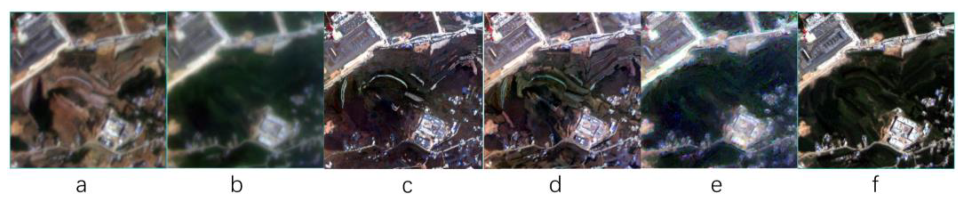
3.2. The Accuracy of Mountains

Study area 2 is mainly a mountainous area. The ground objects in the basic image obtained on 15 April 2021 are mainly cultivated land, buildings, and roads. In the image obtained on 10 July 2021, the original cultivated land has undergone the process of crop coverage changes (Figure 3a,b). The original PS image can roughly identify the ground object information, but its resolution is still somewhat insufficient for the identification of more detailed information. According to the effect of the spatiotemporal fusion algorithm, the three models have better fusion effects on ground objects, and the identification of ground object information is obviously more accurate. The FSDAF algorithm and STDFA algorithm have higher fusion image accuracy, but the fusion image displays a poor response to changes in crop coverage (Figure 3c,d). Generally speaking, the fusion image and the verification image should have the similar spectral, but the color of the two models in the crop coverage area is quite different from that of the verification image. Fortunately, we were still able to distinguish vegetation cover areas by color comparisons. In terms of resolution, both models can clearly display the spatial structure information of ground objects; in particular, the land structure in the vegetation-covered area can be better observed. Compared with the original PS image, the spatial resolution of the fusion image is also improved to a certain extent, the contours of different types of objects are also clearer, and the changes in the coverage areas of crops can be better displayed (Figure 3e). However, its resolution in specific spatial details is slightly lower than that of the other two algorithms.

From the statistical analysis results (

Table 3. The fusion accuracy evaluation of different bands for different models.

Band	Method	CC	SSIM	RMSE	AAD
Blue	FSDAF	0.6437	0.4863	0.2899	0.0653
	STDFA	0.7335	0.5013	0.0787	0.0652
	Fit_FC	0.7588	0.5590	0.0605	0.0445
Green	FSDAF	0.6563	0.6621	0.2817	0.0473
	STDFA	0.7107	0.6763	0.0720	0.0469
	Fit_FC	0.7648	0.7171	0.0607	0.0320
Red	FSDAF	0.6920	0.6478	0.2791	0.0288
	STDFA	0.7437	0.6680	0.0688	0.0290
	Fit_FC	0.6658	0.7041	0.0614	0.0230
NIR	FSDAF	0.6214	0.6866	0.2744	0.0115
	STDFA	0.6009	0.6961	0.0672	0.0114
	Fit_FC	0.6658	0.6760	0.0641	0.0171
Mean	FSDAF	0.6534	0.6207	0.2813	0.0382
	STDFA	0.6972	0.6354	0.0717	0.0381
	Fit_FC	0.7138	0.6641	0.0617	0.0292

), the fusion image of the Fit_FC model has a good correlation with the verification image. With the exception of the red band, the CC value of the Fit_FC model is higher than that of the FSDAF and STDFA models. The average value of CC is 0.7138, which is 0.0605 and 0.0166 higher than that of the FSDAF and STDFA models, respectively, indicating that the spectral similarity between the fusion image and the verification effect is higher. At the same time, the SSIM of the Fit_FC model in the blue, green, and red bands is also higher than that of the FSDAF and STDFA models, with an average of 0.6641, which is 0.0434 and 0.0287 higher than that of the other two models, respectively, indicating that its structural similarity is also higher than that of the other two models. In all four bands, the RMSE value of the FSDAF model is the highest, that of the Fit_FC model is the lowest, and the average values of the three models are 0.0791, 0.0052, and 0.0038 in descending order, indicating that the difference between the fusion image of the FSDAF model and the validation image is greater than others. Regarding the AAD value, the AAD of the FSDAF and STDFA models in the blue, green, and red bands is significantly higher than that of the Fit_FC model, but slightly lower than that of the Fit_FC model in the near-infrared band. The average AAD values of the FSDAF, STDFA, and Fit_FC models were 0.0382, 0.0381, and 0.0291, respectively, indicating that the Fit_FC model had less biased fusion images. The statistical results show that the Fit_FC model has the best fusion effect in mountainous areas, and the FSDAF algorithm has the worst fusion effect.

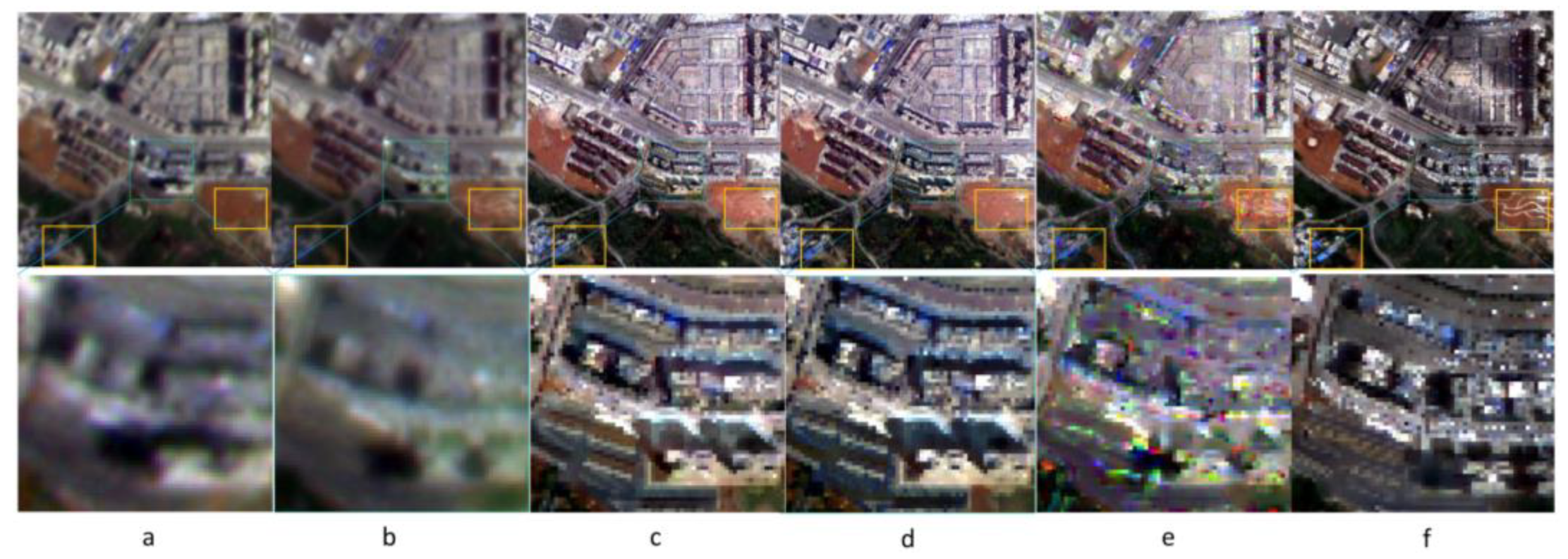
3.3. The Accuracy of Urban

Study area 3 is mainly an urban area, and the types of ground objects in the area are mainly urban buildings, building land, roads, and vegetation greening. In the images from April and July in this area, with the exception of some areas where the land use changed (marked in yellow), the rest of the features changed little (Figure 4a,b). The original PS image can identify different types of objects, but the outlines between buildings are relatively blurred. Through direct observation of the fused image, compared to the PS image, all three models have improved spatial resolution to a certain extent, and can restore the area partially covered by shadows (red border) (Figure 4c–e). Among them, the fusion images of the STDFA and FSDAF models have a higher resolution. Fit_FC is relatively blurry on the outline of the building, and there is a more obvious block effect. For the two land use changes in the image, the fusion results of the STDFA algorithm cannot clearly reflect these. FSDAF is also extremely blurry, mainly following the original base image, making it difficult to effectively identify changes. Relatively speaking, the fusion image of the Fit_FC algorithm can better reflect the difference between the base image and the predicted image, and is more similar to the verification image. However, it does not achieve excellent result for the recognition of building outlines.

According to the statistical analysis results (

Table 4. The fusion accuracy evaluation of different bands for different models.

Band	Method	CC	SSIM	RMSE	AAD
Blue	FSDAF	0.5880	0.7839	0.0449	0.0091
	STDFA	0.5711	0.7835	0.0455	0.0091
	Fit_FC	0.5447	0.7775	0.0467	0.0057
Green	FSDAF	0.5092	0.7382	0.0568	0.0079
	STDFA	0.4850	0.7313	0.0581	0.0079
	Fit_FC	0.4797	0.7451	0.0578	0.0010
Red	FSDAF	0.5775	0.7238	0.0604	0.0073
	STDFA	0.5467	0.7098	0.0626	0.0005
	Fit_FC	0.5768	0.7334	0.0608	0.0030
NIR	FSDAF	0.4989	0.6570	0.0754	0.0057
	STDFA	0.4240	0.6044	0.0806	0.0057
	Fit_FC	0.5436	0.6733	0.0727	0.0053
Mean	FSDAF	0.5434	0.7257	0.0594	0.0075
	STDFA	0.5067	0.7073	0.0617	0.0058
	Fit_FC	0.5362	0.7323	0.0595	0.0038

), the CC values of the three models are generally distributed in the range of 0.5–0.6, and the difference between each band is small; the FSDAF model has the highest CC values in the blue, green, and red bands, and the Fit_FC model has the highest in the near-infrared band. The mean values of CC for the FSDAF, STDFA, and Fit_FC algorithms are 0.5434, 0.5067, and 0.5362, respectively, indicating that the spectral similarity between the fused image and the validation impact is the highest for FSDAF and the lowest for the STDFA model. The SSIM gaps of the FSDAF, STDFA, and Fit_FC models are small, with average values of 0.7257, 0.7072, and 0.7323, respectively, and the Fit_FC model has the highest SSIM values in the green, red, and near-infrared bands, indicating that the structural similarity between the fusion image and the verification image is better. The RMSE value of the STDFA model is higher than that of the FSDAF and Fit_FC models in the green, red, and near-infrared bands, and the average values of the three models are 0.0040, 0.0036, and 0.0036, respectively, indicating that the STDFA model has a larger error in fused images. At the same time, the average AAD values of the three models of FSDAF, STDFA, and Fit_FC are 0.0075, 0.0058, and 0.0038, respectively, indicating that the fusion image deviation of the FSDAF model is large. In general, although the FSDAF model has the highest AAD, its fusion image still has a good prediction effect.

4. Discussion

Different spatiotemporal fusion models have different fusion effects in karst areas. In order to select a more appropriate high-resolution data fusion model under different scenarios and needs, in this paper, the fusion results of the three models in different karst landforms are directly observed and statistically analyzed, and the application effects of the three models in karst areas are discussed.

4.1. FSDAF in Different Regions

The fusion image of the FSDAF model can improve the resolution of the original image and the classification accuracy of surface land use in three geomorphic types (water land border, mountain area, and urban area). Among them, the FSDAF model has a good fusion effect in the land water border area. It can not only clearly identify the water boundary, but it can also effectively identify information such as shoals. Therefore, the FSDAF model can be used for spatiotemporal fusion of target lakes, oceans, rivers, and other waters, and can accurately extract the water boundary. This advantage has important value in flood relief, remote danger monitoring of dammed lakes, and other practical applications. The FSDAF model has a large color difference between the fusion image and the verification image in mountainous areas and other areas with large seasonal changes in vegetation cover. The vegetation coverage cannot be restored well. The FSDAF model can effectively improve the resolution of urban areas. It can more effectively identify the building outline, and more effectively display the part of the original image that is blocked by shadows. However, similar to the integration performance of mountain areas, the model cannot well show the land type change in the building area. This may be because the FSDAF model mainly uses spatial prediction to retrieve pixel changes. Theoretically, spatial prediction can truly describe the surface information of the predicted date. In addition, the signals of land cover type change and local variation are retained in the fusion results [26]. However, in the actual process, the error of FSDAF mainly depends on the residual distribution under the assumption of surface uniformity. Therefore, the FSDAF model can save more detailed information through this strategy, but it limits its ability to retrieve land cover changes.

4.2. STDFA in Different Regions

The STDFA model also has a good fusion effect on the images of different landforms in karst areas, which can effectively improve the image resolution. The STDFA model has a good recognition ability in the interface area between water and land, but the accuracy of fusion results is not high due to the appearance of “patches” in the predicted image. Different from this, the fusion image resolution of the STDFA model in mountainous areas is very high, which can better identify the structural information between ground objects. However, the fusion accuracy of the STDFA model is lower than that of the Fit_FC model in areas with large changes in vegetation cover such as crops. However, based on the statistical data, the CC and SSIM of each band of the STDFA model are lower than that of the FSDAF model, while RMSE is higher than that of the FSDAF model. This indicates that in urban areas, the fusion accuracy of the STDFA model is lower than that of the FSDAF model. In addition, the STDFA model is a spatiotemporal fusion model based on the unmixing method, and its data fusion accuracy is related to two aspects: On the one hand, the STDFA model needs to classify high-resolution data in the basic period, but the classification accuracy of unsupervised classification methods (such as K-means method) will cause the fusion accuracy to decrease. On the other hand, when the resolution difference between high-resolution low-temporal data and high-temporal low-resolution data is large, the area represented by each high-resolution pixel will be more refined. For example, in the pixels of high-temporal and low-resolution data, when the richness of a certain category is very low, the fitting error will increase [48,49].

4.3. Fit_FC in Different Regions

The fusion accuracy of the Fit_FC model in different geomorphic types in karst area is quite different. The fusion effect of the Fit_FC model is poor at the interface between land and water. Compared with the original low-spatial-resolution measurement data on 10 July 2021, the spatial resolution is not significantly improved, and it is difficult to identify the boundary between water surface and land. Meanwhile, the statistical results of the Fit_FC model also show that the fusion accuracy is extremely low, and the correlation coefficient of the green band is as low as 0.12466. Therefore, the Fit_FC model is not suitable for image fusion at the interface between land and water. The Fit_FC model has a good fusion result in the mountainous area. The spatial resolution of the image is improved, and the changes of vegetation cover such as crops can be better presented. It is very suitable for spatiotemporal fusion in areas with large vegetation changes and increases the accuracy of ground class classification. Therefore, the Fit_FC model can be given priority when studying the requirements of vegetation dynamic monitoring and land use change. The fusion results of the Fit_FC model have lower resolution than the FSDAF and STDFA models in the contour of ground objects such as roads and buildings. Especially in densely built areas, the resolution gap is larger. In addition, the Fit_FC model fits the high-temporal and low-resolution data of the known and predicted periods at pixel scale, and directly applies the fitting coefficients to the high-resolution and low-temporal data. When the difference between high-resolution data and low-resolution data is large, the results of the Fit_FC model show obvious “block effect” [28,50].

4.4. Statistical Precision Analysis

For the fusion effect of the three models in different regions, it is found that the resolution is generally good in direct observation, but the statistical data of the related accuracy are obviously not high, being clearly lower than that of the related low-resolution data. This is due to the high resolution of the two sets of data that we use, which can accurately identify small changes in ground objects. Especially when the prediction data and the verification data are separated by three days, the information on the ground objects, such as vehicles, will be slightly different, and some land types will also change. At the same time, in the process of the spatiotemporal fusion of high-resolution variable images, the effect of sunlight will also have a great impact on the accuracy. Differences in shooting time, different satellite shooting angles, and changes in the incident angle of sunlight will cause the shadow areas of the basic image and the verification image to differ, which will have a certain impact on the analysis of statistical data. Under the combined effect of these factors, the fusion accuracy of the three algorithms for high-resolution data is lower than the fusion of the same model for medium- and low-resolution data. However, in general, in most cases, the resolution of the fused image becomes higher, the recognizability is greatly enhanced, and the practical application value is higher.

4.5. Classification Accuracy Verification

In order to verify the application accuracy of the fusion results in land use classification, we selected an area containing mountains, buildings, and waters for research. First, the three methods are applied to different land use types for spatiotemporal integration. Secondly, the fusion results are divided into forest land, dry land, construction land, and water through the supervised classification method. Finally, through the comparison with the data of the Third National Land Survey of China (TNLS), it can be seen from Figure 5 and

Table 5. Comparison between classification results and TNLS data.

Land Use	Classification (km2)	TNLS (km2)	D-Value (km2)	Ratio
Dry land	1.1301	1.3901	−0.2600	81.29%
Water	2.7325	2.6749	0.0576	102.15%
Forest land	1.0585	0.937	0.1215	112.96%
Construction land	3.1611	3.0801	0.0810	102.63%

that the classification results of the fused images (Figure 5a) are highly consistent with the data of the TNLS of China (Figure 5b). However, compared with the data of TNLS, the classification results did not effectively divide the small area of water around the construction land region, which made the water area in the classification results smaller. For forest land and dry land, the classification results are scattered. At the same time, due to the time difference between the fusion image and TNLS, the original dry land is distributed with crops, which makes the classification result of the fusion image become forest land. This may result in the increase of forest land area and the decrease of dry land area. For construction land, the area may be increased due to construction activities. However, the classification results are basically consistent with the data of TNLS. In general, the classification result of the fusion image is good, and the difference of land area of each type is within 15%. Therefore, images fused by spatiotemporal fusion model can be used for land use classification.

5. Conclusions

In this study, three simple and easy-to-promote spatiotemporal fusion models, FSDAF, STDFA, and Fit_FC, are selected to fuse GF-2 and PS high-resolution satellite data. Four classical evaluation indexes, SSIM, CC, RMSE, and AAD, and visual analysis are adopted. The applicability of the three models for land use classification in karst areas is discussed comprehensively. The results show that the three models can improve the accuracy of land surface recognition, but the accuracy is different in different land use types. Among them, the fusion results of the FSDAF model can improve the recognition accuracy of land and water interface. Different from the FSDAF model, the STDFA model has the highest resolution of fusion image in mountain region, with significant improvement of fusion image resolution and rich details. The fusion effect of the Fit_FC model is poor in the boundary region of water and land. The image is blurred, and the ground feature information cannot be restored clearly, which is not conducive to the classification of land and water boundary land use. However, the Fit_FC model can clearly show land use change in vegetation covered areas. Therefore, this paper adopts a high-resolution spatiotemporal fusion algorithm to effectively improve the classification of land use in karst areas. It is of great significance to optimize the allocation of land resources and realize ecological restoration in fragile karst mountainous areas.

References

1. Febles-Gonzalez, J.M.; Vega-Carreno, M.B.; Tolon-Becerra, A.; Lastra-Bravo, X. Assessment of soil erosion in karst regions of Havana, Cuba. Land Degrad. Dev. 2012, 23, 465–474. [Google Scholar] [CrossRef]
2. Zhang, S.R.; Bai, X.Y.; Zhao, C.W.; Tan, Q.; Luo, G.J.; Wang, J.F.; Li, Q.; Wu, L.H.; Chen, F.; Li, C.J.; et al. Global CO2 consumption by silicate rock chemical weathering: Its past and future. Earth’s Futur. 2021, 9, e2020EF001938. [Google Scholar] [CrossRef]
3. Li, Q.; Wang, S.; Bai, X.; Luo, G.; Song, X.; Tian, Y.; Hu, Z.; Yang, Y.; Tian, S. Change Detection of Soil Formation Rate in Space and Time Based on Multi Source Data and Geospatial Analysis Techniques. Remote Sens. 2020, 12, 121. [Google Scholar] [CrossRef] [Green Version]
4. Li, C.J.; Bai, X.Y.; Tan, Q.; Zhao, C.W.; Luo, G.J.; Wu, L.H.; Chen, F.; Xi, H.P.; Luo, X.L.; Ran, C.; et al. High-resolution mapping of the global silicate weathering carbon sink and its long-term changes. Glob. Change Biol. 2022, 28, 4377–4394. [Google Scholar] [CrossRef] [PubMed]
5. Zhang, S.R.; Bai, X.Y.; Zhao, C.W.; Tan, Q.; Luo, G.J.; Wu, L.H.; Xi, H.P.; Li, C.J.; Chen, F.; Ran, C.; et al. China’ s carbon budget inventory from 1997 to 2017 and its challenges to achieving carbon neutral strategies. J. Clean. Prod. 2022, 347, 130966. [Google Scholar] [CrossRef]
6. Gong, S.H.; Wang, S.J.; Bai, X.Y.; Luo, G.J.; Zeng, C. Response of the weathering carbon sink in terrestrial rocks to climate variables and ecological restoration in China. Sci. Total Environ. 2020, 750, 141525. [Google Scholar] [CrossRef] [PubMed]
7. Chen, F.; Bai, X.; Liu, F.; Luo, G.; Tian, Y.; Qin, L.; Li, Y.; Xu, Y.; Wang, J.; Wu, L.; et al. Analysis Long-Term and Spatial Changes of Forest Cover in Typical Karst Areas of China. Land 2022, 11, 1349. [Google Scholar] [CrossRef]
8. Roy, D.P.; Ju, J.; Lewis, P.; Schaaf, C.; Gao, F.; Hansen, M.; Lindquist, E. Multi-temporal MODIS–Landsat data fusion for relative radiometric normalization, gap filling, and prediction of Landsat data. Remote Sens. Environ. 2008, 112, 3112–3130. [Google Scholar] [CrossRef]
9. Gevaert, C.M.; García-Haro, F.J. A comparison of STARFM and an unmixing-based algorithm for Landsat and MODIS data fusion. Remote Sens. Environ. 2015, 156, 34–44. [Google Scholar] [CrossRef]
10. Liao, C.; Wang, J.; Pritchard, I.; Liu, J.; Shang, J. A Spatio-Temporal Data Fusion Model for Generating NDVI Time Series in Heterogeneous Regions. Remote Sens. 2017, 9, 1125. [Google Scholar] [CrossRef]
11. Guan, X.; Liu, G.; Huang, C.; Liu, Q.; Wu, C.; Jin, Y.; Li, Y. An Object-Based Linear Weight Assignment Fusion Scheme to Improve Classification Accuracy Using Landsat and MODIS Data at the Decision Level. IEEE Trans. Geosci. Remote Sens. 2017, 55, 6989–7002. [Google Scholar] [CrossRef]
12. Chen, B.; Ge, Q.; Fu, D.; Yu, G.; Sun, X.; Wang, S.; Wang, H. A data-model fusion approach for upscaling gross ecosystem productivity to the landscape scale based on remote sensing and flux footprint modelling. Biogeosciences 2010, 7, 2943–2958. [Google Scholar] [CrossRef] [Green Version]
13. Zhang, H.K.; Huang, B.; Zhang, M.; Cao, K.; Yu, L. A generalization of spatial and temporal fusion methods for remotely sensed surface parameters. Int. J. Remote Sens. 2015, 36, 4411–4445. [Google Scholar] [CrossRef]
14. Wei, J.; Wang, L.; Liu, P.; Chen, X.; Li, W.; Zomaya, A.Y. Spatiotemporal Fusion of MODIS and Landsat-7 Reflectance Images via Compressed Sensing. IEEE Trans. Geosci. Remote Sens. 2017, 55, 7126–7139. [Google Scholar] [CrossRef]
15. Ju, J.; Roy, D.P. The availability of cloud-free Landsat ETM+ data over the conterminous United States and globally. Remote Sens. Environ. 2008, 112, 1196–1211. [Google Scholar] [CrossRef]
16. Mizuochi, H.; Hiyama, T.; Ohta, T.; Fujioka, Y.; Kambatuku, J.R.; Iijima, M.; Nasahara, K.N. Development and evaluation of a lookup-table-based approach to data fusion for seasonal wetlands monitoring: An integrated use of AMSR series, MODIS, and Landsat. Remote Sens. Environ. 2017, 199, 370–388. [Google Scholar] [CrossRef]
17. Song, H.; Huang, B. Spatiotemporal Satellite Image Fusion Through One-Pair Image Learning. IEEE Trans. Geosience Remote Sens. 2013, 51, 1883–1896. [Google Scholar] [CrossRef]
18. Liu, J.; Fan, X.; Jiang, J.; Liu, R.; Luo, Z. Learning a Deep Multi-scale Feature Ensemble and an Edge-attention Guidance for Image Fusion. IEEE Trans. Circuits Syst. Video Technol. 2021, 32, 105–119. [Google Scholar] [CrossRef]
19. Zhu, X.; Cai, F.; Tian, J.; Williams, T.K.-A. Spatiotemporal Fusion of Multisource Remote Sensing Data: Literature Survey, Taxonomy, Principles, Applications, and Future Directions. Remote Sens. 2018, 10, 527. [Google Scholar] [CrossRef] [Green Version]
20. Wu, B.; Huang, B.; Cao, K.; Zhuo, G. Improving spatiotemporal reflectance fusion using image inpainting and steering kernel regression techniques. Int. J. Remote Sens. 2017, 38, 706–727. [Google Scholar] [CrossRef]
21. Amorós-López, J.; Gómez-Chova, L.; Alonso, L.; Guanter, L.; Zurita-Milla, R.; Moreno, J.; Camps-Valls, G. Multitemporal fusion of Landsat/TM and ENVISAT/MERIS for crop monitoring. Int. J. Appl. Earth Obs. Geoinf. 2013, 23, 132–141. [Google Scholar] [CrossRef]
22. Zhang, W.; Li, A.; Jin, H.; Bian, J.; Zhang, Z.; Lei, G.; Qin, Z.; Huang, C. An Enhanced Spatial and Temporal Data Fusion Model for Fusing Landsat and MODIS Surface Reflectance to Generate High Temporal Landsat-Like Data. Remote Sens. 2013, 5, 5346–5368. [Google Scholar] [CrossRef] [Green Version]
23. Hwang, T.; Song, C.; Bolstad, P.V.; Band, L.E. Downscaling real-time vegetation dynamics by fusing multi-temporal MODIS and Landsat NDVI in topographically complex terrain. Remote Sens. Environ. 2011, 115, 2499–2512. [Google Scholar] [CrossRef]
24. Huang, B.; Song, H. Spatiotemporal reflectance fusion via sparse representation. IEEE Trans. Geosci. Remote Sens. 2012, 50, 3707–3716. [Google Scholar] [CrossRef]
25. Zhu, X.; Helmer, E.H.; Gao, F.; Liu, D.; Chen, J.; Lefsky, M.A. A flexible spatiotemporal method for fusing satellite images with different resolutions. Remote Sens. Environ. Interdiscip. J. 2016, 172, 165–177. [Google Scholar] [CrossRef]
26. Wang, Q.M.; Atkinson, P.M. Spatio-Temporal Fusion for Daily Sentinel-2 Images. Remote Sens. Environ. 2018, 204, 31–42. [Google Scholar] [CrossRef] [Green Version]
27. Li, Y.; Ren, Y.; Gao, W.; Jia, J.; Tao, S.; Liu, X. An enhanced spatiotemporal fusion method–Implications for DNN based time-series LAI estimation by using Sentinel-2 and MODIS. Field Crops Res. 2022, 279, 108452. [Google Scholar] [CrossRef]
28. Qiao, X.; Yang, G.; Shi, J.; Zuo, Q.; Liu, L.; Niu, M.; Wu, X.; Ben-Gal, A. Remote Sensing Data Fusion to Evaluate Patterns of Regional Evapotranspiration: A Case Study for Dynamics of Film-Mulched Drip-Irrigated Cotton in China’s Manas River Basin over 20 Years. Remote Sens. 2022, 14, 3438. [Google Scholar] [CrossRef]
29. Zhang, H.; Huang, F.; Hong, X.; Wang, P. A Sensor Bias Correction Method for Reducing the Uncertainty in the Spatiotemporal Fusion of Remote Sensing Images. Remote Sens. 2022, 14, 3274. [Google Scholar] [CrossRef]
30. Chen, R.; Li, X.; Zhang, Y.; Zhou, P.; Wang, Y.; Shi, L.; Jiang, L.; Ling, F.; Du, Y. Spatiotemporal Continuous Impervious Surface Mapping by Fusion of Landsat Time Series Data and Google Earth Imagery. Remote Sens. 2021, 13, 2409. [Google Scholar] [CrossRef]
31. Morgan, B.E.; Chipman, J.W.; Bolger, D.T.; Dietrich, J.T. Spatiotemporal Analysis of Vegetation Cover Change in a Large Ephemeral River: Multi-Sensor Fusion of Unmanned Aerial Vehicle (UAV) and Landsat Imagery. Remote Sens. 2021, 13, 51. [Google Scholar] [CrossRef]
32. Luo, Y.; Guan, K.; Peng, J.; Wang, S.; Huang, Y. STAIR 2.0: A Generic and Automatic Algorithm to Fuse Modis, Landsat, and Sentinel-2 to Generate 10 m, Daily, and Cloud-/Gap-Free Surface Reflectance Product. Remote Sens. 2020, 12, 3209. [Google Scholar] [CrossRef]
33. Zhou, C.W.; Yang, R.; Yu, L.F.; Zhang, Y.; Yan, L.B. Hydrological and ecological effects of climate change in Caohai watershed based on SWAT model. Appl. Ecol. Environ. Res. 2019, 17, 161–172. [Google Scholar] [CrossRef]
34. Wu, J.; Yang, H.; Yu, W.; Yin, C.; He, Y.; Zhang, Z.; Xu, D.; Li, Q.; Chen, J. Effect of Ecosystem Degradation on the Source of Particulate Organic Matter in a Karst Lake: A Case Study of the Caohai Lake, China. Water 2022, 14, 1867. [Google Scholar] [CrossRef]
35. Yang, K.; Yu, Z.; Luo, Y.; Zhou, X.; Shang, C. Spatial-temporal variation of lake surface water temperature and its driving factors in Yunnan-Guizhou Plateau. Water Resour. Res. 2019, 55, 4688–4703. [Google Scholar] [CrossRef]
36. Xiao, L.; Chen, X.; Zhang, R.; Zhang, Z. Spatiotemporal Evolution of Droughts and Their Teleconnections with Large-Scale Climate Indices over Guizhou Province in Southwest China. Water 2019, 11, 2104. [Google Scholar] [CrossRef] [Green Version]
37. Lian, Y.Q.; You, G.J.Y.; Lin, K.R.; Jiang, Z.C.; Zhang, C.; Qin, X.Q. Characteristics of climate change in southwest China karst region and their potential environmental impacts. Environ. Earth Sci. 2014, 74, 937–944. [Google Scholar] [CrossRef]
38. Li, W.; Jiang, J.; Guo, T.; Zhou, M.; Tang, Y.; Wang, Y.; Zhang, Y.; Cheng, T.; Zhu, Y.; Cao, W.; et al. Generating Red-Edge Images at 3 M Spatial Resolution by Fusing Sentinel-2 and Planet Satellite Products. Remote Sens. 2019, 11, 1422. [Google Scholar] [CrossRef] [Green Version]
39. Kwan, C.; Zhu, X.; Gao, F.; Chou, B.; Perez, D.; Li, J.; Shen, Y.; Koperski, K.; Marchisio, G. Assessment of spatiotemporal fusion algorithms for planet and worldview images. Sensors 2018, 18, 1051. [Google Scholar] [CrossRef] [PubMed] [Green Version]
40. Ren, K.; Sun, W.; Meng, X.; Yang, G.; Du, Q. Fusing China GF-5 Hyperspectral Data with GF-1, GF-2 and Sentinel-2A Multispectral Data: Which Methods Should Be Used? Remote Sens. 2020, 12, 882. [Google Scholar] [CrossRef]
41. Ren, J.; Yang, W.; Yang, X.; Deng, X.; Zhao, H.; Wang, F.; Wang, L. Optimization of Fusion Method for GF-2 Satellite Remote Sensing Images based on the Classification Effect. Earth Sci. Res. J. 2019, 23, 163–169. [Google Scholar] [CrossRef] [Green Version]
42. Zhang, D.; Xie, F.; Zhang, L. Preprocessing and fusion analysis of GF-2 satellite Remote-sensed spatial data. In Proceedings of the 2018 International Conference on Information Systems and Computer Aided Education (ICISCAE), Changchun, China, 6–8 July 2018; IEEE: Piscataway, NJ, USA, 2018; pp. 24–29. [Google Scholar]
43. Zhu, X.; Chen, J.; Gao, F.; Chen, X.; Masek, J.G. An enhanced spatial and temporal adaptive reflectance fusion model for complex heterogeneous regions. Remote Sens. Environ. 2010, 114, 2610–2623. [Google Scholar] [CrossRef]
44. Jia, D.; Cheng, C.; Song, C.; Shen, S.; Ning, L.; Zhang, T. A Hybrid Deep Learning-Based Spatiotemporal Fusion Method for Combining Satellite Images with Different Resolutions. Remote Sens. 2021, 13, 645. [Google Scholar] [CrossRef]
45. Tang, Y.; Wang, Q.; Zhang, K.; Atkinson, P. Quantifying the Effect of Registration Error on Spatio-temporal Fusion. IEEE J. Sel. Top. Appl. Earth Obs. Remote Sens. 2020, 13, 487–503. [Google Scholar] [CrossRef] [Green Version]
46. Cheng, F.; Fu, Z.; Tang, B.; Huang, L.; Huang, K.; Ji, X. STF-EGFA: A Remote Sensing Spatiotemporal Fusion Network with Edge-Guided Feature Attention. Remote Sens. 2022, 14, 3057. [Google Scholar] [CrossRef]
47. Hou, S.; Sun, W.; Guo, B.; Li, C.; Li, X.; Shao, Y.; Zhang, J. Adaptive-SFSDAF for Spatiotemporal Image Fusion that Selectively Uses Class Abundance Change Information. Remote Sens. 2020, 12, 3979. [Google Scholar] [CrossRef]
48. Wu, M.; Niu, Z.; Wang, C.; Wu, C.; Wang, L. Use of MODIS and Landsat time series data to generate high-resolution temporal synthetic Landsat data using a spatial and temporal reflectance fusion model. J. Appl. Remote Sens. 2012, 6, 063507. [Google Scholar]
49. Wu, M.; Wu, C.; Huang, W.; Niu, Z.; Wang, C.; Li, W.; Hao, P. An Improved High Spatial and Temporal Data Fusion Approach for Combining Landsat and MODIS Data to Generate Daily Synthetic Landsat Imagery. Inf. Fusion 2016, 31, 14–25. [Google Scholar] [CrossRef]
50. Liu, M.; Ke, Y.; Yin, Q.; Chen, X.; Im, J. Comparison of Five Spatio-Temporal Satellite Image Fusion Models over Landscapes with Various Spatial Heterogeneity and Temporal Variation. Remote Sens. 2019, 11, 2612. [Google Scholar] [CrossRef]
Figure 1. Location of the study region. (1) Land–water boundary area, (2) mountainous area, (3) urban area.
Land 12 00033 g001
Figure 2. (a) PS image on 15 April; (b) PS image on 10 July; (c) fusion image by FSDAF on 10 July; (d) fusion image by STDFA on 10 July; (e) fusion image by Fit_FC on 10 July; (f) GF-2 verification image on 13 July.
Land 12 00033 g002
Figure 3. (a) PS image on 15 April; (b) PS image on 10 July; (c) fusion image by FSDAF on 10 July; (d) fusion image by STDFA on 10 July; (e) fusion image by Fit_FC on 10 July; (f) GF-2 verification image on 13 July.
Land 12 00033 g003
Figure 4. (a) PS image on 15 April; (b) PS image on 10 July; (c) fusion image by FSDAF on 10 July; (d) fusion image by STDFA on 10 July; (e) fusion image by Fit_FC on 10 July; (f) GF-2 verification image on 13 July.
Land 12 00033 g004
Figure 5. (a) Supervise classification results; (b) Data of China’s Third National Land Survey.
Land 12 00033 g005