Article

Lacustrine Urban Blue Spaces: Low Availability and Inequitable Distribution in the Most Populated Cities in Mexico

Laboratorio de Restauración Ecológica, Instituto de Biología, Universidad Nacional Autónoma de México, Ciudad de Mexico 04510, Mexico
*
Author to whom correspondence should be addressed.
Land 2023, 12(1), 228; https://doi.org/10.3390/land12010228
Submission received: 8 December 2022 / Revised: 5 January 2023 / Accepted: 5 January 2023 / Published: 11 January 2023

Abstract

:
Lacustrine blue spaces provide benefits to the urbanites and wildlife habitat. Their availability varies depending on the city in which they are established and intra-urban social interactions. We analyzed the presence, distribution, and size of lentic water bodies in Mexico’s 145 most populated cities. We searched for patterns in their distribution concerning demographic, socioeconomic, and geographic data, aiming to understand their socio-ecological interactions in cities. We digitized lacustrine spaces to obtain their number per city, total surface, area of blue space per inhabitant, and surface as a percentage of the city’s total area. We tested for relationships between their number and surface and city population, hydrological regions, and urban marginalization index through linear and generalized linear models. We delimited 1834 lacustrine blue spaces, finding almost two-thirds of them artificial. Their presence and surface in Mexican cities were generally low, except for hydrological regions close to the Gulf of Mexico. Their number and surface decreased as the urban marginalization index increased. The lack of equitable provision of lacustrine space at the national level has implications for urban planning and land management. Blue spaces should maximize their ecosystem services’ provision for the whole society to promote cities’ sustainability and resilience.

1. Introduction

Lacustrine blue spaces are currently inherent elements of cities since human populations have settled near, along, around, and even above lakes, lagoons, and other lentic and lotic water bodies to fulfill their basic needs of water, feeding, and waste disposal [1,2]. In growing cities, these blue spaces are modified and engulfed by settlements. In the absence of natural spaces, artificial lacustrine blue spaces are built for the benefit of the population [1,3,4]. Like urban green spaces, and often in synergy with them, blue spaces provide habitat for urban wildlife species [5,6], and several ecosystem services for urbanites [7,8], among which are urban heat island effect mitigation [9,10,11], rainwater retention [7], tourism and recreation linked to aesthetical and landscape values [7,12], and the favoring of overall wellbeing [7,13,14,15,16].
In the current times of Global Climate Change, blue spaces and green spaces can be regarded as part of nature-based solutions aiming to mitigate its adverse effects on cities [7,17,18]. Blue spaces have gained importance in recent years in the face of the increasing droughts affecting the water supply in urban areas. At the same time, cities face flooding with risks to people’s safety [19]. Therefore, blue spaces within cities are managed or created to provide critical ecosystem services to the population [9]. Nonetheless, the demand for these services from blue spaces is usually high and immediate due to cities’ characteristic high concentration of population [20]. Additionally, blue spaces were, and still are, used for residential and industrial wastewater disposal [21,22]. Consequently, many of them are currently neglected, eutrophicated, and polluted [23,24,25].
The ecological condition of blue spaces can be a source of disservices and risks to health and safety for people interacting with them, such as bad seasonal smell or the presence of mosquitoes; vectors of diseases such as dengue, zika, and chikungunya [6]. In rainy seasons, poorly managed blue spaces can contribute to flooding with damage to infrastructure and people, mainly in low-income areas [26,27,28]. Furthermore, while initially, blue spaces were a source of drinking water and food, as they became waste dumps, their capacity to offer provision services was limited or lost [29,30]. Perceived often as wastelands [31], blue spaces are highly vulnerable since they have been, and are, systematically desiccated for their conversion to other urban land uses [1,2,21]. Nevertheless, their vulnerability level and the services and disservices they provide are closely linked to their seasonality, condition, planning, and management [1,13,26,32]. Lacustrine blue spaces’ vulnerability and disturbance are due to the high demographic concentration in cities, the incorporation of rural spaces into irregular settlements, garbage dumping, wastewater discharge, and the intermittency of the water bodies themselves [1,4,33], favoring hence their invasion and allowing construction to take place in their beds, or even causing its utter disappearance.
Despite their importance and vulnerability, knowledge of the presence, water quality, and social appraisal of blue spaces, albeit in continuous growth in the last few years, is still limited; many of their ecological, biological, and sociocultural aspects (e.g., use, biodiversity) are unknown for most cities [29,32], a situation that for Mexico is no exception [1]. Even so, the few studies about Mexican lacustrine urban blue spaces highlight the need for research, actions, and good practices, from different approaches, leading to their restoration. These actions should be aimed at the conservation of the biological groups that live in these habitats and for the benefit of the citizens [1,5,21,34]. There is a feedback loop between human activities and blue spaces; humans affect the ecological functions of blue spaces, and in turn, blue spaces influence the urban environment, sociocultural interactions, and public health [1]. Consequently, these spaces’ study, management, restoration, and conservation need to be addressed with disciplines and approaches from natural and social sciences and available biotechnological advances [35,36,37]. These loop interactions are relevant to the sustainability and resilience of cities [1,13,26,32].
Aiming to understand the socioecological role of lacustrine blue spaces in cities, we pose the following questions: (1) what is the availability of lacustrine blue spaces in cities settled in contrasting ecosystems; (2) how artificial are these spaces in cities, and what are their main uses; (3) what is their distribution pattern within cities throughout a country with similar urban development; and (4) is the distribution of lacustrine blue spaces associated with geography and geomorphology or with socioeconomic variables such as urban marginalization? To answer these questions, in this study, we analyzed the presence, distribution, and size of natural and artificial lacustrine blue spaces (lakes and ponds, mainly; [38]), together with demographic, socioeconomic, and geographic data to identify the relevance of such factors on the blue spaces in the most populated cities of Mexico. Mexico as a study system can help to answer such questions since it is a country with contrasting environmental conditions (hydrological, climatological, geomorphological, eco-systemic; [39,40,41]), and a high percentage of urban population with profound socio-economical differences [42,43,44]. Yet, on a national scale, it shares a political regime and a normative framework under which cities are planned and managed [45,46].
Given the dynamics of loss and gain of lacustrine blue spaces [2,4,17], we expected most of them in Mexican cities to be artificial with predominantly recreational use [3]. It is widely reported that green and blue-green spaces are distributed heterogeneously through the urban territory associated with higher-income urban areas [47,48,49,50,51], so we expected lacustrine blue spaces to be negatively associated with the population in most marginalized zones similarly. If this is the case, it would indicate an inequitable distribution [52,53] regarding lacustrine blue spaces and the services they provide in the most populated cities in Mexico.

2. Materials and Methods

To fulfill the study aims, we followed a spatially explicit approach and GIS mapping at the national scale of the current state and dynamics of the lacustrine blue spaces as biophysical elements of the urban environment [54]. The study was performed in 145 urban localities with more than 100,000 inhabitants in Mexico, according to the 2020 Population and House Census [55] (Table S1; Figure 1). For the limits of cities, we used the polygons from the National Geostatistical Mark for the same Census [56]. We identified and manually delimited lacustrine blue spaces within the cities’ polygons in Google Earth Pro version 7.3 for pc (https://www.google.es/earth/, accessed on 29 October 2021) on the imagery mosaics available from dates January 2017 to October 2021 (spanning five years of both dry and rainy seasons). In some cases, 2017 images were the most recent images available. No space was digitized on older imagery. We identified lacustrine blue spaces visually with the help of the time bar and the zoom tools. We digitized the blue space polygons using the polygon tool following the visible margins of water. The lacustrine blue spaces we considered and delimited here were mainly ponds, lakes, lagoons, wetlands, dams, and other water reservoirs, including some water treatment plants. We did not consider swimming pools, sediment ponds, most fountains, rivers, or streams. We neither include blue spaces located outside the borders of cities. All digitized lacustrine blue spaces were saved in a Keyhole Markup Language Zipped (.kmz) file, which we transformed into a shape file (.shp) to compute the attributes of blue spaces on each city in QGIS v.3.16 [57].
For each lacustrine blue space, we calculated its surface based on delimited polygons (including in the accounting, in many cases, the islands within the lakes) and recorded, if possible, its use, the land use where it was emplaced (e.g., parks, residential areas), and if the space was natural (pre-existent water body, generally modified and engulfed by the settlements) or artificial (built for the benefit of the population). In the case of multi-spaces, each part was considered as one entity. We also recorded in which of the following Hydrological Regions the lacustrine blue spaces were located: Baja California Peninsula, North, Pacific, Center, Gulf, and Yucatan Peninsula. These six major regions correspond to the simplified recategorization of the 37 Hydrological Regions from the National Water Commission [58].

2.1. Blue Spaces Indicators per City

For each city, we obtained and analyzed the distribution of (1) the number of blue spaces, (2) the total surface of blue spaces, (3) the area (m2) of blue spaces per inhabitant, and (4) the percentage surface that blue spaces represent of the city extension, as basic indicators to evaluate urban blue infrastructure, following the subjacent rationale than that for urban green spaces [59,60]. We elaborated the corresponding maps for each indicator to show their nationwide distribution in Mexico in QGIS v.3.16 [57]. Information layers and maps had a Lambert Conformal Conic Projection and Ellipsoid GRS80, the same as the National Geostatistical Mark from INEGI [56] we used for delimitations of cities.

2.2. Blue Space’s Relationship with City Population and Hydrological Regions

To test the relevance of population and hydrological regions on the number of lacustrine blue spaces, we carried out a generalized linear model (GLM) with the quasi-Poisson family due to the overdispersion of our data [61]. To evaluate the relevance of those same variables on the lacustrine blue spaces surface, we performed a GLM with the Gamma family (identity link). For this latter case, we specify the dependent variable as lacustrine blue spaces surface plus one (i.e., hectares +1). For both cases, we specify the cities’ population per ten thousand inhabitants and sorted hydrological regions in descending order according to their accounted total surface of blue spaces (i.e., Gulf, Center, North, Pacific, Yucatan Peninsula, and Baja California Peninsula).

2.3. Blue Spaces by Urban Marginalization Index

We further evaluated the relationship between the number and surface of lacustrine blue spaces and the urban marginalization index (UMI) of the National Council of Population (CONAPO by its acronym in Spanish) for 2020 [62]. The UMI is calculated, based on population and housing census data, to evaluate “the shortages suffered by the population as a result of lack of access to education and health, residence in inadequate housing, and lack of assets.” [63] (p. 1). It consists of five marginalization levels: ‘very low’, ‘low’, ‘medium’, ‘high’, and ‘very high’. This index is estimated at the spatial unit of urban basic geostatistical area (AGEB by its acronym in Spanish); each urban AGEB is a group of 25 to 50 blocks delimited by streets, avenues, and trails, with residential, industrial, services, or commercial land use [64]. Since the analysis must only be calculated for AGEBs with at least 20 private inhabited dwellings with information on their occupants [63], there were AGEBs for which UMI was unavailable. For such AGEBs, we used the label ‘no data’. We also evaluated the differences in the average number of blue spaces by the level of UMI via a GLM using the quasi-Poisson family. For the relationship between the surface of lacustrine blue spaces and the UMI, we used a linear model (LM) specifying the dependent variable (hectares) in a logarithmic scale to adjust for non-normality and heterogeneity of variance [65]. As an alternative to the pairwise comparison, and given the ordinal nature of the UMI, instead of the default dummy coding contrasts in R, which compares the mean of each level to the reference mean level; we carried out backward difference coding contrasts, to compare adjacent levels of the UMI (each level minus the previous level [66]). For these analyses involving the UMI, we excluded the ‘no data’ AGEBs. For the models, we obtained the explained variance D2 and adjusted R2 for GLMs and LM, respectively [65,67]. For models using the log of the variable or link = log (LM and quasi-Poisson GLMs, respectively), we present the coefficients of the models as well as the percent change ([exp(coefficient) − 1 × 100]; [68]) for such coefficients. Additionally, we carried out a Chi-squared test and a mosaic plot [65] to test for associations between the type of space where blue spaces were emplaced and the UMI. We performed all of the statistical analyses in R [69] and considered the results significant at p values ≤ 0.05. We depict the general flux of methods for blue spaces analysis in Figure 2.

3. Results

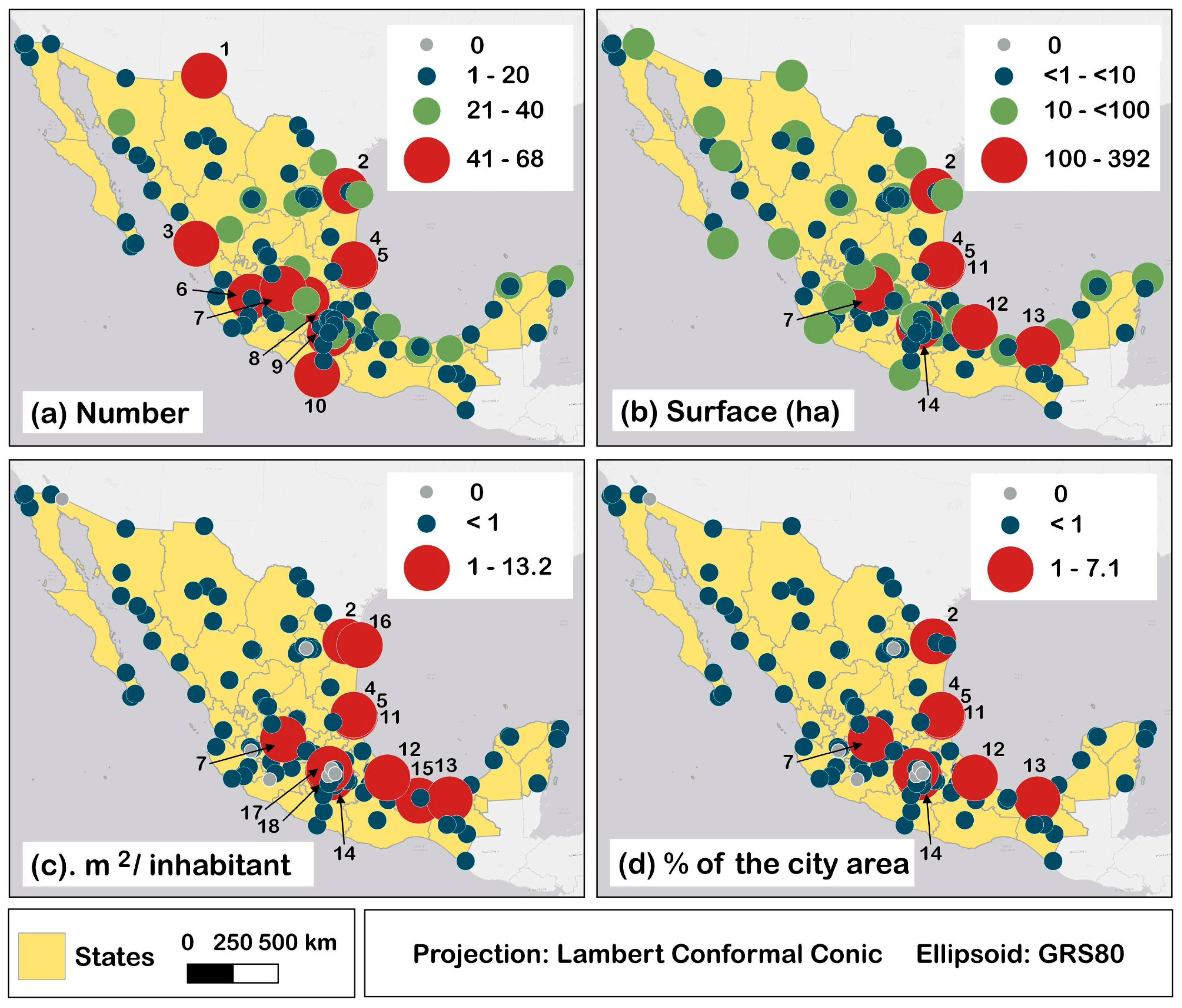
3.1. Blue Spaces from the Most Populated Mexican Cities

We delimited 1834 lacustrine blue spaces, whose surfaces sum up to 2836.1 ha, varying from 0.001 to 319.2 ha, showing an average surface of 1.5 (±11.7 SD) ha. However, the median value was 0.2 ha. 75.5% of lacustrine blue spaces had a surface < 0.5 ha, and only ten (0.5%) blue spaces measured more than 50 ha. We identified 1257 (68.5%) blue spaces as artificial systems, 51 (2.8%) as natural systems, and for the rest, 526 (28.7%), we could not determine if they were artificial or natural. Almost one-third of lacustrine blue spaces were in golf courses, followed by green spaces (e.g., parks, zoos, botanical gardens, institutional green spaces), residential areas, and dams. For half of the spaces, we could not precisely define the type of space in which they were located (Figure 3a). Regarding their use, we identified most blue spaces as recreational (including for landscaping purposes), and for water storage for a later purpose, a minimum of spaces showed other use (e.g., ornamental fish production; boat sheltering). For a high proportion of spaces, we could not identify their use (Figure 3b).

3.2. Blue Spaces per City

The 1834 blue spaces were from 137 urban areas; in eight of the 145 cities, we did not record the presence of visible lacustrine urban blue spaces. The range of the number of blue spaces in cities was 0–68, with an average of 12.6 (±14.6 SD; median = 8) blue spaces per city. Blue spaces surface varied among cities, from 0 to 392.3 ha and the average was 19.6 (±54.9 SD; median = 3 ha) ha. For the index of m2 of blue spaces per inhabitant in cities, values varied from 0 to 13.2 m2/inhabitant, with an average of 0.5 (±1.6 SD; median = 0.1) m2/inhabitant. The percentage that surfaces of blue spaces represent of the cities’ extension ranged from 0 up to 7.1%, showing an average of 0.3 (±0.9 SD; median = 0.1) %. Distributions of these indicators showed a heavy positive skewness (with median values much lower than average values). This distribution indicates that most Mexican cities had low values of blue spaces attributes, and very few cities had high values (Figure 4). Only ten cities had more than 40 lacustrine blue spaces within their territories, and eight cities had blue spaces surfaces that summed up ≥1 km2. Twelve were the cities with ≥1 m2 of blue spaces per inhabitant, and nine were the cities whose surface of blue spaces represents more than 1% of the city’s extension (Figure 5). We show each city’s estimated blue spaces indicators in the Supplementary Material (Table S1).

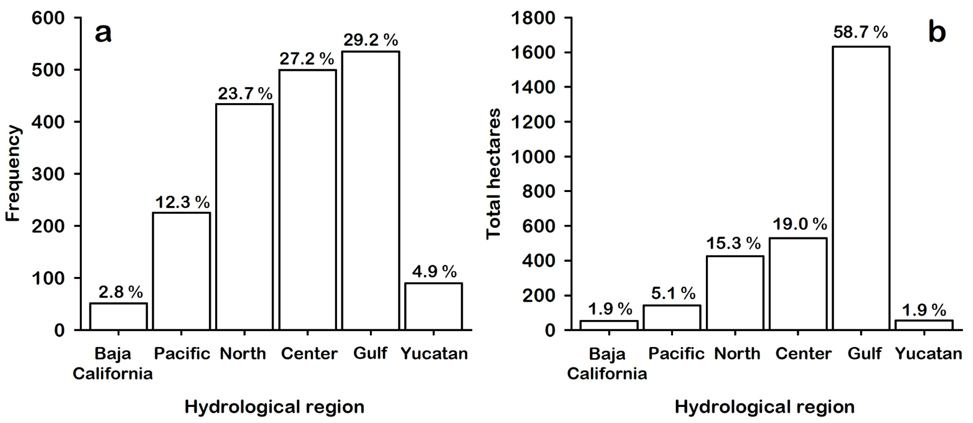
3.3. Blue Spaces’ Relationship with Hydrological Regions and City Population

Regarding hydrological regions, there were few blue spaces on both Mexican Peninsulas, with an increase in number from the Pacific, North, Center, and Gulf (Figure 6a). Despite the Gulf region showing the highest total number of blue spaces, it had the second lowest average, after the Baja California Peninsula. The region with the highest average number of blue spaces was the Center, followed by the Yucatan Peninsula, the North, and the Pacific regions, respectively (Table 1). The quasi-Poisson model results indicated a positive and significant relationship between the number of blue spaces and population in cities, albeit with a very low coefficient, and pointed out that, except for the Baja California region, the rest of the regions had non-significant higher numbers of blue spaces than the Gulf region. The explained variance for the model was 18.92% (Table 2). As for blue spaces’ surface, almost 60% was in the Gulf region, and the remaining percentage was distributed in the other hydrological regions (Figure 6b). Mean surface values of blue spaces by region varied from 53.59 and 54.02 ha for the Peninsulas up to 1632.09 ha for the Gulf region (Table 1). The GLM (Gamma family, identity link) showed a positive and significant relationship between the population and lacustrine blue spaces surface with a coefficient of 0.346 per 10,000 inhabitants. On the other hand, the Center, North, Pacific, and the Peninsulas of Yucatan and Baja California showed negative and significant coefficients, indicating that blue spaces in the cities of the Gulf hydrological region are undeniably higher than in the rest of the regions. The percent of variance explained by the model for the surface of lacustrine blue spaces was 29.91% (Figure 6b, Table 3).

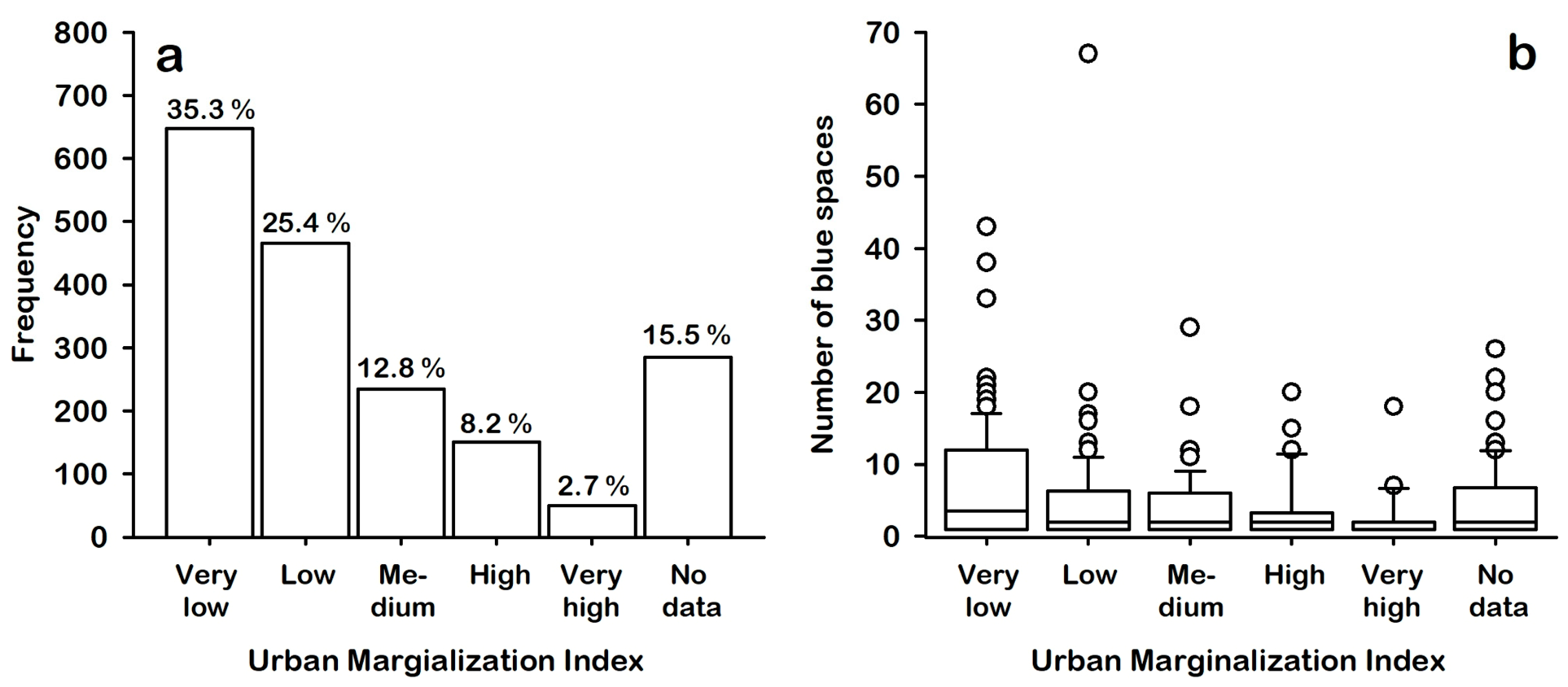
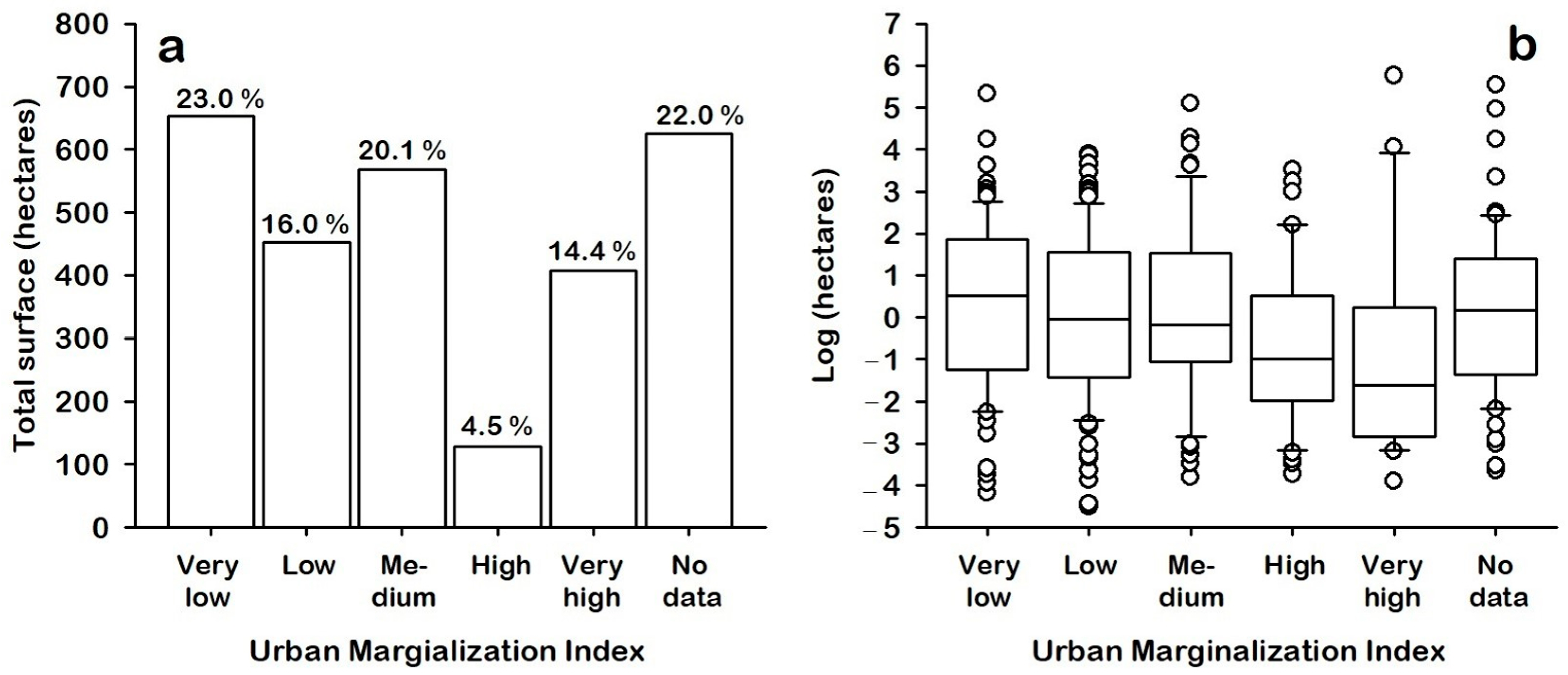
3.4. Blue Spaces by Urban Marginalization Index

Of the total recorded number of lacustrine blue spaces in the 145 most populated Mexican cities, 35% were on ‘very low’ marginalization AGEBs, and the percentage decreased to only 2.7% of these spaces in the ‘’very high’ marginalization areas (Figure 7a). According to the quasi-Poisson GLM results, not all levels of the UMI had the same mean number of blue spaces. A change in the UMI level led to a change in the number of lacustrine blue spaces. Results from the backward contrast indicated that all contrasts were negative, nonetheless only the ‘low’–‘very low’ contrast was significant (Figure 7b, Table 4). This means that the relation between the number of blue spaces in AGEBs and the urban marginalization index was negative. It is less likely to find blue spaces in the more marginalized zones than in those of less marginalization.
Almost 60% of lacustrine blue spaces’ total surface (ha) was in AGEBs of ‘medium’ to ‘very low’ marginalization. Near 20% was in AGEBs of ‘high’ and ‘very high’ marginalization; the remaining percent was in AGEBs where no UMI was computed because they do not meet the minimum population and housing criteria for performing the analysis (Figure 8a). Results of LM showed a significant negative relationship between the log hectares of lacustrine blue spaces and the five levels of UMI (F4, 298 = 2.479, p = 0.044). According to backward contrast, the surface of the blue spaces of levels (log form) was lower than that of their previous adjacent levels, except for the ‘medium’-‘low’ contrast. However, the only significant (p < 0.05) result was between ‘high’ and ‘medium’ (Table 5; Figure 8b). This indicates that AGEBs of ‘high’ and ‘very high’ marginalization have lower surfaces than those of ‘medium’ to ‘very low’ marginalization. The explained variances of models for the number and surface of lacustrine blue spaces concerning UMI were low, albeit lower for the surface model than that for the number of blue spaces (Table 4 and Table 5).
Finally, the Chi-squared test showed a significant relationship between UMI and the type of space where blue spaces were located (Chi220 = 437, p < 0.0001). Larger proportions of golf courses than expected were associated with the ‘very low’ marginalization areas and lower proportions than expected with the rest of the UMI levels; green spaces were associated with ‘low’ marginalization AGEBs, dams to ‘medium’ marginalization, and undefined blue spaces to ‘medium’ to ‘very high’ marginalization zones (Figure 9).

4. Discussion

Blue spaces are part of the identities of cities worldwide and are significant for population and wildlife [7,70,71]. Lacustrine blue spaces are integral components of Mexican cities, yet their overall availability was low in number and extension for most cities, being their distribution associated with the country’s contrasting geographic and socioeconomic traits. Furthermore, most recorded Mexican lacustrine blue spaces were artificial, with only a small fraction of them being natural yet having a larger surface. The low number of natural urban blue spaces suggests that just a few cities have incorporated lakes, lagoons, and other lentic water bodies as they have settled and grown, and most have built these spaces. At a national level, these tendencies are consistent with previous findings on the assessment of natural and artificial blue spaces since Iojă et al. [59] reported low availability of blue spaces in Romania, and Darrah et al. [3] documented the decline of natural spaces and the increase in artificial ones from 1970 to 2015 on a global scale and in Latin America. These significant differences between the proportions of artificial and natural lacustrine blue spaces are associated with the existence of this contradictory practice of desiccation of natural spaces and, at the same time, the generation of artificial ones. In Mexico, this practice can be traced back to the foundation and establishment of the current Mexico City on Lake Texcoco and others from the same lacustrine system [2]. Lacustrine blue spaces in Mexican cities are modified and mainly constructed to fulfill recreational and leisure activities and provide other cultural ecosystem services for the population [12,72,73,74,75]. The ecological and environmental services provided by lacustrine urban spaces [7,74,76] are becoming recognized as they can be considered nature-based solutions to address environmental and social challenges in the current times [13,18,77].
As being intertwined with green spaces [6,19], the association of a higher number and surface of lacustrine blue spaces with less marginalized zones in cities is in line with the studies showing an inequitable distribution of green, blue-green, and blue spaces across cities’ territories, often associated with variables that reflect wealthier conditions [50,78,79,80,81,82,83]. Furthermore, as being mainly artificial, blue spaces in golf courses contribute to an increase in the total number of blue spaces in Mexican cities, with both positive and negative ecological and economic outcomes [84,85]. However, their presence was highly associated with zones of very low marginalization. This implies that while blue spaces in golf courses are valuable for biodiversity and their ecological services [86,87], the cultural services they provide are only directly accessible to the segment of the population that can afford their admission [88,89]. Consequently, their benefits for the rest of the population are indirect, as, for example, that derived from tourism [90].
The uneven distribution of natural and artificial blue spaces availability in the most populated cities of Mexico associated with the less marginalized zones could indicate, at least, a distributive environmental injustice [51,53] regarding urban lacustrine blue spaces. Distributive environmental injustice is widely reported for public space, albeit mainly for green spaces, including explanations of its causes and aspects of accessibility [47,49,51,53,91]. For both natural and artificial lacustrine spaces, it seems that corresponding local authorities and real estate developers have favored and oriented their interest and efforts, to fulfill the requirements of the wealthier sectors of the population in Mexican cities nationwide. However, further studies at local and national scales are needed on distributive environmental justice for urban blue spaces, as well as on the other dimensions of environmental justice as procedural and interactional [53,92]. In terms of planning and management of cities and their blue and green spaces, achieving an equitable distribution is not only about generating more spaces or providing more surface area, but about ensuring available and accessible spaces of quality, and the services they provide, to all people, including vulnerable groups and minorities, also according to their needs [52,53,83,93,94,95].
The geographic attributes of the country also drove the distribution of lacustrine blue spaces. The Gulf Hydrological Regions have the highest total values for the four indicators by city evaluated. In this region are the six cities with the largest blue spaces of natural origin, which account for almost 45% of the total surface of the recorded lacustrine blue spaces. This region has the highest annual total mean natural surface runoff [96] since several of the country’s largest rivers flow into the Gulf side of the country. Yet, the total number and surface of lacustrine blue spaces in cities from the Pacific Region were relatively low considering that this has the second highest annual total mean natural surface runoff yet representing only 35% of that from the Gulf Region.
Furthermore, only 17 studied cities were in the Pacific region, contrasting with the 51 in the Gulf. In the North and Center regions are all the dams we recorded, contributing to a higher surface in cities from those regions in comparison with both Peninsulas, which have the lowest values of lacustrine blue spaces number and surface, as having the lowest annual runoff, also. While the presence and surface of lacustrine blue spaces are associated with the hydrological diversity of Mexico, other geographic variables could contribute to the variation in their distribution as orography (i.e., plains, plateau, hills, mountain basins), which has shown to have an influence on blue spaces surface in other countries [59]. Variations in altitude, climate regions, or vegetation regions on blue spaces attributes and distribution in Mexico remain to be tested.
Regarding city population size, the number and the surface of lacustrine blue spaces increased as the cities’ population increased. Nonetheless, the quasi-Poison and Gamma models’ coefficients were very low per 10,000 inhabitants, and the deviances explained were also low, indicating that the model could be improved by including other explanatory variables [65]. Beyond the statistical implications of the models, these suggest a low availability of lacustrine blue spaces for the people in the most populated cities in Mexico, which was also evident from the values obtained of the indices of m2 of blue spaces per inhabitant and the percentage that these spaces represent from the cities surface. A similar tendency for both these indices is reported by Iojă et al. [59] for blue spaces in Romania on a nationwide scale.

Limitations and Opportunities

We here focused on lacustrine blue spaces in the Mexican cities of more than 100,000 inhabitants, yet information is necessary about smaller cities or peri-urban blue spaces, which, given their nearness to the cities’ boundaries, are affected by their growth and metabolism. We found that most Mexican cities have at least one lacustrine blue space, for most of which their condition and many aspects about them are unknown (e.g., levels of pollution and eutrophication, ecosystem services they provide in their current state, who are the beneficiaries of such services, which spaces are sources of risks or diseases to population), which need to be studied at local and regional scales. From the 145 studied cities, there are studies on water quality and biodiversity of lacustrine blue spaces, for only a few of them, as is the case of Villahermosa and Tampico, located in the Gulf hydrological region with the larger natural lakes and lagoons [21,25,34,97,98,99], Mexico City, with large natural blue spaces and numerous small artificial ones [23,100,101,102,103], and Cuernavaca and Puebla in the Center hydrological region [5,104].
In a small fraction of the studied cities, we did not detect the presence of lacustrine blue spaces. Nonetheless, this does not mean that those cities do not have blue spaces but that they may not have been detectable, either because they were dry or because they were surrounded by vegetation or other covers that hid the water mirrors, on which our study is primarily based, during the period of study. This, in turn, is related to blue spaces seasonality, a factor for variation in the data since water mirrors change their size depending on the season [38]. Therefore, the size and presence of lacustrine blue spaces in cities can vary depending on the date (of satellite images) on which measures were taken. In this case, available images were from January 2017 to October 2021, spanning dry and rainy seasons throughout the country. In some cases, images from 2017 were the most recent images available on Google Earth. In this sense, temporal studies are necessary to update the status of blue spaces’ presence, surface, and other variables [59], including their establishment or incorporation history into cities through an intensive compiling of complementary sources of suitable information (e.g., older satellite imagery, orthophotos, older pictures, historical maps and documents).
Through available satellite imagery, we can only infer some of the information on the lacustrine blue spaces, like land use of their location, their use, and whether they are natural or artificial, the reason why field work is necessary to establish those variables as accurately as possible, as well as on physical, chemical, and biological aspects, water depth, quality, and supply. Once collecting information for the high number of blue spaces for which we could not identify if they were natural or artificial, nor the land use where they are located or their predominant use, our results will vary. The polygon used as city delimitation and the quality of the satellite image (cloud cover, pixel size) also added variability to the obtained results.
Blue spaces’ indicators need to be considered and complemented with other indicators as those of green spaces to offer a general view of their availability in cities on a national scale [59]. Some information on their presence, location, surface, and number per city can be extracted from the INEGI website, from the section hydrography (https://www.inegi.org.mx/temas/hidrografia/ accessed on 20 October 2021), and the digital Map of Mexico at http://gaia.inegi.org.mx/mdm6/ (accessed on 22 October 2021), also from INEGI, nonetheless, the information for some urban areas appears incomplete, mainly for artificial spaces. It would be worthwhile to address the magnitude of coherence or inconsistency between official and satellite image-derived information, considering the seasonality of blue spaces and dates of the information gathering [59]. While this is, to our knowledge, one of the first studies with an overview to understand blue spaces on a national scale, more in-depth studies can and need to be generated. There is still a wide range of opportunities for the study of the state and both positive and negative aspects of urban blue spaces from diverse disciplines such as biology, ecology, political sciences, anthropology, sociology, legislation, planning, management, restoration, hydrology, and others, considering them as spaces of social and ecological importance for the population wellbeing and the resilience of cities.

5. Conclusions

Lacustrine blue spaces are inherent elements of Mexican cities; however, even though a high percentage of them are artificial, their availability in number and surface is low nationwide. Such a low availability derives in both low values of m2 per inhabitant and coverage percentages of the cities. Lacustrine blue spaces appear inextricably intertwined with green spaces such as parks of several types and golf courses, and to a lesser extent with residential green spaces. Hence, the main apparent use that such spaces fulfill in cities is recreational and scenic. In other words, they function mainly as providers of cultural ecosystem services. Blue spaces are unevenly distributed across the most populated Mexican cities in association with geographic and socioeconomic conditions since it is more likely to find more and larger blue spaces in cities along the Gulf of Mexico hydrological region and areas of low marginalization. This could be an indication of distributive environmental injustice for lacustrine blue species among and within the most populated cities in Mexico. Further studies on urban blue spaces’ physical, chemical, ecological, biological, and sociocultural aspects are necessary, both temporally and spatially, at local, regional, and national scales, including aspects of procedural and interactional environmental justice. Along with green spaces, lacustrine blue spaces should be considered and attended to in cities’ planning and management agendas to increase their equitable provision of services, the resilience of both lacustrine blue spaces and the cities, and as a pathway for urban sustainability.

Supplementary Materials

The following supporting information can be downloaded at: https://www.mdpi.com/article/10.3390/land12010228/s1, Table S1: Estimated lacustrine blue spaces indicators in Mexican cities for 2021.

Author Contributions

Conceptualization, I.F. and L.Z.; methodology, I.F. and L.Z.; validation, I.F.; formal analysis, I.F.; investigation, I.F.; data curation, I.F.; writing—original draft preparation, I.F.; writing—review and editing, I.F. and L.Z.; visualization, I.F.; supervision, L.Z.; funding acquisition, I.F. and L.Z. All authors have read and agreed to the published version of the manuscript.

Funding

This research was funded by Universidad Nacional Autónoma de México through postdoctoral research support for IF from “Postdoctoral Fellowship Program at the National Autonomous University of Mexico” (“Programa de Becas Posdoctorales en la Universidad Nacional Autónoma de México”).

Data Availability Statement

Datasets for this research are included in this paper, its Supplementary Materials, and references.

Acknowledgments

IF acknowledges and appreciates the support for postdoctoral research from the “Postdoctoral Fellowship Program at the National Autonomous University of Mexico” (“Programa de Becas Posdoctorales en la Universidad Nacional Autónoma de México”).

Conflicts of Interest

The authors declare no conflict of interest. The funders had no role in the design of the study; in the collection, analyses, or interpretation of data; in the writing of the manuscript; or in the decision to publish the results.

References

  1. Molina-Prieto, L.F.; Rubio Fernández, D. Elementos de urbanismo azul: Lagos naturales y artificiales. Rev. Investig. 2016, 9, 22–44. [Google Scholar] [CrossRef]
  2. Poó Rubio, A. Origen es Destino. La Ciudad de México. De la Ciudad Lacustre a la Metrópoli de los Desastres Hídricos. In Proceedings of the XI Encuentro Iberoamericano de Mujeres Ingenieras, Arquitectas y Agrimensoras, Santo Domingo, Dominican Republic, 5–10 March 2012; p. 36. [Google Scholar]
  3. Darrah, S.E.; Shennan-Farpón, Y.; Loh, J.; Davidson, N.C.; Finlayson, C.M.; Gardner, R.C.; Walpole, M.J. Improvements to the Wetland Extent Trends (WET) Index as a Tool for Monitoring Natural and Human-Made Wetlands. Ecol. Indic. 2019, 99, 294–298. [Google Scholar] [CrossRef]
  4. Forman, R.T.T. Urban Ecology: Science of Cities; Cambridge University Press: New York, NY, USA, 2014. [Google Scholar]
  5. Almazán-Núñez, R.C.; Hinterholzer-Rodríguez, A. Dinámica temporal de la avifauna en un parque urbano de la ciudad de Puebla, México. Huit. Rev. Mex. Ornitol. 2010, 11, 26–34. [Google Scholar] [CrossRef]
  6. Gledhill, D.G.; James, P. Rethinking Urban Blue Spaces from a Landscape Perspective: Species, Scale and the Human Element. In Ecological Perspectives of Urban Green and Open Spaces; Breuste, J., Ed.; Salzburger Geographische Arbeiten: Salzburg, Austria, 2008; Volume 42, pp. 151–164. [Google Scholar]
  7. Haase, D. Reflections about Blue Ecosystem Services in Cities. Sustain. Water Qual. Ecol. 2015, 5, 77–83. [Google Scholar] [CrossRef]
  8. Lemes de Oliveira, F. Eco-Cities: The Role of Networks of Green and Blue Spaces. In Cities for Smart Environmental and Energy Futures: Impacts on Architecture and Technology; Rassia, S.T., Pardalos, P.M., Eds.; Energy Systems; Springer: Berlin/Heidelberg, Germany, 2014; pp. 165–178. [Google Scholar]
  9. Gunawardena, K.R.; Wells, M.J.; Kershaw, T. Utilising Green and Bluespace to Mitigate Urban Heat Island Intensity. Sci. Total Environ. 2017, 584–585, 1040–1055. [Google Scholar] [CrossRef] [PubMed]
  10. Shi, D.; Song, J.; Huang, J.; Zhuang, C.; Guo, R.; Gao, Y. Synergistic Cooling Effects (SCEs) of Urban Green-Blue Spaces on Local Thermal Environment: A Case Study in Chongqing, China. Sustain. Cities Soc. 2020, 55, 102065. [Google Scholar] [CrossRef]
  11. Völker, S.; Baumeister, H.; Claßen, T.; Hornberg, C.; Kistemann, T. Evidence for the Temperature-Mitigating Capacity of Urban Blue Space—A Health Geographic Perspective. Erdkunde 2013, 67, 355–371. [Google Scholar] [CrossRef]
  12. Chaudhry, P.; Bhargava, R.; Sharma, M.P.; Tewari, V.P. Conserving Urban Lakes for Tourism and Recreation in Developing Countries: A Case from Chandigarh, India. Int. J. Leis. Tour. Mark. 2013, 3, 267–281. [Google Scholar] [CrossRef]
  13. Andersson, E.; Langemeyer, J.; Borgström, S.; McPhearson, T.; Haase, D.; Kronenberg, J.; Barton, D.N.; Davis, M.; Naumann, S.; Röschel, L.; et al. Enabling Green and Blue Infrastructure to Improve Contributions to Human Well-Being and Equity in Urban Systems. BioScience 2019, 69, 566–574. [Google Scholar] [CrossRef]
  14. Garrett, J.K.; White, M.P.; Huang, J.; Ng, S.; Hui, Z.; Leung, C.; Tse, L.A.; Fung, F.; Elliott, L.R.; Depledge, M.H.; et al. Urban Blue Space and Health and Wellbeing in Hong Kong: Results from a Survey of Older Adults. Health Place 2019, 55, 100–110. [Google Scholar] [CrossRef]
  15. Nutsford, D.; Pearson, A.L.; Kingham, S.; Reitsma, F. Residential Exposure to Visible Blue Space (But Not Green Space) Associated with Lower Psychological Distress in a Capital City. Health Place 2016, 39, 70–78. [Google Scholar] [CrossRef]
  16. Völker, S.; Kistemann, T. The Impact of Blue Space on Human Health and Well-Being—Salutogenetic Health Effects of Inland Surface Waters: A Review. Int. J. Hyg. Environ. Health 2011, 214, 449–460. [Google Scholar] [CrossRef] [PubMed]
  17. Mankikar, S.; Driver, B. Blue-Green Infrastructure: An Opportunity for Indian Cities. Obs. Res. Found. Occas. Pap. 2021, 317, 1–38. [Google Scholar]
  18. Kabisch, N.; Frantzeskaki, N.; Pauleit, S.; Naumann, S.; Davis, M.; Artmann, M.; Haase, D.; Knapp, S.; Korn, H.; Stadler, J.; et al. Nature-Based Solutions to Climate Change Mitigation and Adaptation in Urban Areas: Perspectives on Indicators, Knowledge Gaps, Barriers, and Opportunities for Action. Ecol. Soc. 2016, 21, 39. [Google Scholar] [CrossRef] [Green Version]
  19. Ghofrani, Z.; Sposito, V.; Faggian, R. A Comprehensive Review of Blue-Green Infrastructure Concepts. Int. J. Environ. Sustain. 2017, 6, 15–36. [Google Scholar] [CrossRef]
  20. Elmqvist, T.; Setälä, H.; Handel, S.; van der Ploeg, S.; Aronson, J.; Blignaut, J.; Gómez-Baggethun, E.; Nowak, D.; Kronenberg, J.; de Groot, R. Benefits of Restoring Ecosystem Services in Urban Areas. Curr. Opin. Environ. Sustain. 2015, 14, 101–108. [Google Scholar] [CrossRef] [Green Version]
  21. Batres González, J.J.; Ortells Chabrera, V.; Lorenzo Palomera, J. Diseño y ordenamiento de la dinámica urbana, medio ineludible en la preservación sustentable de los de los recursos hídricos naturales urbanos en México, caso lagunas urbanas del sur de Tamaulipas (Tampico-Madero-Altamira). Quivera 2010, 12, 1–13. [Google Scholar]
  22. Ricárdez de la Cruz, G.; López Ocaña, G.; Bautista Margulis, R.G.; Torres Balcázar, C.A. Laguna de las Ilusiones y su entorno urbano: Aguas residuales, urbanas y sedimentos. Kuxulkab’ 2016, 22, 27–38. [Google Scholar] [CrossRef]
  23. Oliva Martínez, M.G.; Rodríguez Rocha, A.; Lugo Vázquez, A.; Sánchez Rodríguez, M. del R. Composición y Dinámica Del Fitoplancton En Un Lago Urbano Hipertrófico. Hidrobiológica 2008, 18, 1–13. [Google Scholar]
  24. Pineda-Mendoza, R.; Martínez-Jerónimo, F.; Garduño-Solórzano, G.; Olvera-Ramírez, R. Caracterización morfológica y molecular de cianobacterias filamentosas aisladas de florecimientos de tres lagos urbanos eutróficos de la Ciudad de México. Polibotánica 2011, 31, 31–50. [Google Scholar]
  25. Rodríguez Rodríguez, E.; Ruíz Ruíz, M.; Vertíz Pérez, L.A. Procesos de Eutroficación en Siete Lagunas Urbanas de Villlahermosa, Tabasco, México. In Proceedings of the Congreso Regional de AIDIS para Norteamérica y El Caribe, San Juan, Puerto Rico, 8–12 June 1997; p. 10. [Google Scholar]
  26. Haeffner, M.; Jackson-Smith, D.; Buchert, M.; Risley, J. Accessing Blue Spaces: Social and Geographic Factors Structuring Familiarity with, Use of, and Appreciation of Urban Waterways. Landsc. Urban Plan. 2017, 167, 136–146. [Google Scholar] [CrossRef]
  27. O’Donnell, E.; Thorne, C.; Ahilan, S.; Arthur, S.; Birkinshaw, S.; Butler, D.; Dawson, D.; Everett, G.; Fenner, R.; Glenis, V.; et al. The Blue-Green Path to Urban Flood Resilience. Blue-Green Syst. 2020, 2, 28–45. [Google Scholar] [CrossRef] [Green Version]
  28. Sánchez González, D. Precipitaciones extremas y sus implicaciones en procesos de remoción en masa en la planificación urbana de Tampico, México. Cuad. Geográficos 2011, 48, 135–159. [Google Scholar]
  29. Joosse, S.; Hensle, L.; Boonstra, W.J.; Ponzelar, C.; Olsson, J. Fishing in the City for Food—A Paradigmatic Case of Sustainability in Urban Blue Space. NPJ Urban Sustain. 2021, 1, 1–8. [Google Scholar] [CrossRef]
  30. Quimby, B.; Crook, S.E.S.; Miller, K.M.; Ruiz, J.; Lopez-Carr, D. Identifying, Defining and Exploring Angling as Urban Subsistence: Pier Fishing in Santa Barbara, California. Mar. Policy 2020, 121, 104197. [Google Scholar] [CrossRef]
  31. Ibrahim, I.; Aminudin, N.; Young, M.A.; Yahya, S.A.I. Education for Wetlands: Public Perception in Malaysia. Procedia-Soc. Behav. Sci. 2012, 42, 159–165. [Google Scholar] [CrossRef] [Green Version]
  32. Birch, S.; McCaskie, J. Shallow Urban Lakes: A Challenge for Lake Management. In The Ecological Bases for Lake and Reservoir Management; Harper, D.M., Brierley, B., Ferguson, A.J.D., Phillips, G., Eds.; Springer: Dordrecht, The Netherlands, 1999; pp. 365–377. [Google Scholar]
  33. Izazola, H. Agua y sustentabilidad en la Ciudad de México. Estud. Demográficos Urbanos 2001, 16, 285. [Google Scholar] [CrossRef]
  34. Pablo-Rodríguez, N.; Olivera-Gómez, L.D. Situación de una población aislada de Manatíes Trichechus manatus (Mammalia: Sirenia: Trichechidae) y conocimiento de la gente, en una laguna urbana, en Tabasco, México. Univ. Cienc. 2012, 28, 15–26. [Google Scholar]
  35. Balvanera, P.; Astier, M.; Gurri, F.D.; Zermeño-Hernández, I. Resiliencia, vulnerabilidad y sustentabilidad de sistemas socioecológicos en México. Rev. Mex. Biodivers. 2017, 88, 141–149. [Google Scholar] [CrossRef]
  36. Salas-Zapata, W.A.; Ríos-Osorio, L.A.; Castillo, J.Á.-D. Bases conceptuales para una clasificación de los sistemas socioecológicos de la investigación en sostenibilidad. Rev. Lasallista Investig. 2012, 8, 7. [Google Scholar]
  37. Urquiza Gómez, A.; Cadenas, H. Sistemas socio-ecológicos: Elementos teóricos y conceptuales para la discusión en torno a vulnerabilidad hídrica. Ordin. Am. 2015, 218, 1–22. [Google Scholar] [CrossRef]
  38. Cervantes, M. Conceptos Fundamentales sobre Ecosistemas Acuáticos y Su Estado en México. In Perspectivas Sobre Conservación de Ecosistemas Acuáticos en México; Sánchez, O., Herzig, M., Peters, E., Márquez-Huitzil, R., Zambrano, L., Eds.; Secretaría de Medio Ambiente y Recursos Naturales: Zapopan, Mexico; Instituto Nacional de Ecología: Xalapa, Mexico; U.S. Fish & Wildlife Service: Washington, DC, USA; Unidos para la Conservación, A.C.: Mexico City, Mexico; Universidad Michoacana de San Nicolás Hidalgo: Morelia, Mexico, 2007; pp. 37–67. [Google Scholar]
  39. Coll-Hurtado, A. Nuevo Atlas Nacional de México. Available online: http://www.igeograf.unam.mx/Geodig/nvo_atlas/index.html/mapas_generales.html (accessed on 21 August 2022).
  40. CONABIO (Comisión Nacional para el Conocimiento y Uso de la Biodiversidad). Portal de Información Geográfica—CONABIO. Available online: http://geoportal.conabio.gob.mx/ (accessed on 21 August 2022).
  41. CONAGUA (Comisión Nacional del Agua). Atlas del Agua en México; Comisión Nacional del Agua: Mexico City, Mexico, 2018. [Google Scholar]
  42. Campos-Vazquez, R.; Lustig, N.; Scott, J. Inequality in Mexico: On the Rise Again; WIDER Policy Brief 2018/5; United Nations University, UNU-WIDER: Helsinki, Finland, 2018; pp. 1–2. [Google Scholar]
  43. Esquivel Hernández, G. Extreme Inequality in Mexico. Concentration of Economic and Political Power 2015. Available online: https://is.cuni.cz/studium/predmety/index.php?do=download&did=113954&kod=JMM591 (accessed on 20 August 2022).
  44. The World Bank. Urban Population (% of Total Population). Available online: https://data.worldbank.org/indicator/SP.URB.TOTL.IN.ZS (accessed on 19 August 2022).
  45. Domínguez, J. El Nuevo Esquema de Ordenamiento Territorial y Desarrollo Urbano En México. In Desarrollo Urbano y Metropolitano en México; Sobrino, J., Ugalde, V., Eds.; El Colegio de Mexico A.C.: Mexico City, Mexico, 2019; pp. 543–578. [Google Scholar]
  46. OCDE (Organización para la Cooperación y el Desarrollo Económicos). Estudios de Políticas Urbanas de la OCDE, México, Transformando la Política Urbana y el Financiamiento de la Vivienda. Síntesis del Estudio 2015. Available online: https://www.oecd-ilibrary.org/urban-rural-and-regional-development/oecd-urban-policy-reviews-mexico-2015_9789264227293-en (accessed on 21 August 2022).
  47. Kabisch, N.; Haase, D. Green Justice or Just Green? Provision of Urban Green Spaces in Berlin, Germany. Landsc. Urban Plan. 2014, 122, 129–139. [Google Scholar] [CrossRef]
  48. Nesbitt, L.; Meitner, M.J.; Girling, C.; Sheppard, S.R.J.; Lu, Y. Who Has Access to Urban Vegetation? A Spatial Analysis of Distributional Green Equity in 10 US Cities. Landsc. Urban Plan. 2019, 181, 51–79. [Google Scholar] [CrossRef]
  49. Ojeda-Revah, L. Equidad en el acceso a las áreas verdes urbanas en México: Revisión de literatura. Soc. Ambiente 2021, 24, 1–28. [Google Scholar] [CrossRef]
  50. Thornhill, I.; Hill, M.J.; Castro-Castellon, A.; Gurung, H.; Hobbs, S.; Pineda-Vazquez, M.; Gómez-Osorio, M.T.; Hernández-Avilés, J.S.; Novo, P.; Mesa-Jurado, A.; et al. Blue-Space Availability, Environmental Quality and Amenity Use across Contrasting Socioeconomic Contexts. Appl. Geogr. 2022, 144, 102716. [Google Scholar] [CrossRef]
  51. Zuniga-Teran, A.A.; Gerlak, A.K.; Elder, A.D.; Tam, A. The Unjust Distribution of Urban Green Infrastructure Is Just the Tip of the Iceberg: A Systematic Review of Place-Based Studies. Environ. Sci. Policy 2021, 126, 234–245. [Google Scholar] [CrossRef]
  52. Kim, J.; Lee, K.J.; Thapa, B. Visualizing Fairness: Distributional Equity of Urban Green Spaces for Marginalized Groups. J. Environ. Plan. Manag. 2021, 65, 833–851. [Google Scholar] [CrossRef]
  53. Low, S. Public Space and Diversity: Distributive, Procedural and Interactional Justice for Parks. In The Ashgate Research Companion to Planning and Culture; Young, G., Stevenson, D., Eds.; Ashgate Publishing: London, UK, 2013; pp. 295–310. [Google Scholar]
  54. Harrison, P.A.; Dunford, R.; Barton, D.N.; Kelemen, E.; Martín-López, B.; Norton, L.; Termansen, M.; Saarikoski, H.; Hendriks, K.; Gómez-Baggethun, E.; et al. Selecting Methods for Ecosystem Service Assessment: A Decision Tree Approach. Ecosyst. Serv. 2018, 29, 481–498. [Google Scholar] [CrossRef] [Green Version]
  55. INEGI (Instituto Nacional de Estadística y Geografía). Microdatos del Censo de Población y Vivienda. 2020. Available online: https://www.inegi.org.mx/programas/ccpv/2020/#Microdatos (accessed on 26 February 2021).
  56. INEGI (Instituto Nacional de Estadística y Geografía). Marco Geoestadístico Nacional del Censo de Población y Vivienda. 2020. Available online: https://www.inegi.org.mx/app/biblioteca/ficha.html?upc=889463776079 (accessed on 22 February 2021).
  57. QGIS Development Team. QGIS Geographic Information System. Open Source Geospatial Found. Proj. 2021. Available online: http://qgis.osgeo.org (accessed on 25 December 2021).
  58. CONAGUA (Comisión Nacional del Agua). Regiones Hidrológicas (2020), Escala 1:250000. República Mexicana. 2021. Available online: http://sina.conagua.gob.mx/sina/tema.php?tema=regionesHidrologicas#&ui-state=dialog (accessed on 11 November 2021).
  59. Iojă, C.I.; Badiu, D.L.; Haase, D.; Hossu, A.C.; Niță, M.R. How about Water? Urban Blue Infrastructure Management in Romania. Cities 2021, 110, 103084. [Google Scholar] [CrossRef]
  60. OEPB (Observatorio del Espacio Público de Bogotá). Reporte Técnico de Indicadores de Espacio Público 2019; Departamento Administrativo de la Defensoría del Espacio Público, Alcaldía Mayor de Bogotá, D.C.: Bogotá, Colombia, 2019; p. 30. Available online: https://observatorio.dadep.gov.co/sites/default/files/2019/reporte_tecnico_de_indicadores_de_espacio_publico_2019_baja.pdf (accessed on 24 January 2022).
  61. Zeileis, A.; Kleiber, C.; Jackman, S. Regression Models for Count Data in R. J. Stat. Softw. 2008, 27, 1–25. [Google Scholar] [CrossRef] [Green Version]
  62. CONAPO (Consejo Nacional de Población). Base de Datos del Índice de Marginación Urbana. 2020. Available online: https://www.gob.mx/conapo/documentos/indices-de-marginacion-2020-284372 (accessed on 6 December 2021).
  63. CONAPO (Consejo Nacional de Población). Índice de Marginación Urbana 2020. Nota Técnico-Metodológica. Available online: https://www.gob.mx/cms/uploads/attachment/file/685307/Nota_t_cnica_IMU_2020.pdf (accessed on 10 March 2022).
  64. CONAPO (Consejo Nacional de Población). Índice de Marginación Urbana 2010. 2010. Available online: http://www.sideso.cdmx.gob.mx/documentos/2017/diagnostico/conapo/2010/Indice%20de%20marginacion%20urbana.pdf (accessed on 27 May 2021).
  65. Crawley, M.J. The R Book, 2nd ed.; Wiley: Chichester, UK, 2013. [Google Scholar]
  66. UCLA: Statistical Consulting Group. R Library Contrast Coding Systems for Categorical Variables. Available online: https://stats.oarc.ucla.edu/r/library/r-library-contrast-coding-systems-for-categorical-variables/#backward (accessed on 13 March 2022).
  67. Martínez de Lejarza, J. GLM-Introducción. 2022. Available online: https://www.uv.es/lejarza/eaa/teoria/EAA7%20glm.pdf (accessed on 15 April 2022).
  68. Wooldridge, J. Introductory Econometrics: A Modern Approach; South-Western College: Cincinnati, OH, USA, 2000. [Google Scholar]
  69. R Core Team. R: A Language and Environment for Statistical Computing. 2022. Available online: https://www.r-project.org/ (accessed on 20 June 2022).
  70. Georgiou, M.; Morison, G.; Smith, N.; Tieges, Z.; Chastin, S. Mechanisms of Impact of Blue Spaces on Human Health: A Systematic Literature Review and Meta-Analysis. Int. J. Environ. Res. Public. Health 2021, 18, 2486. [Google Scholar] [CrossRef]
  71. Grellier, J.; White, M.P.; Albin, M.; Bell, S.; Elliott, L.R.; Gascón, M.; Gualdi, S.; Mancini, L.; Nieuwenhuijsen, M.J.; Sarigiannis, D.A.; et al. BlueHealth: A Study Programme Protocol for Mapping and Quantifying the Potential Benefits to Public Health and Well-Being from Europe’s Blue Spaces. BMJ Open 2017, 7, e016188. [Google Scholar] [CrossRef] [Green Version]
  72. Ghermandi, A.; Fichtman, E. Cultural Ecosystem Services of Multifunctional Constructed Treatment Wetlands and Waste Stabilization Ponds: Time to Enter the Mainstream? Ecol. Eng. 2015, 84, 615–623. [Google Scholar] [CrossRef]
  73. Johansson, M.; Pedersen, E.; Weisner, S. Assessing Cultural Ecosystem Services as Individuals’ Place-Based Appraisals. Urban For. Urban Green. 2019, 39, 79–88. [Google Scholar] [CrossRef]
  74. Plieninger, T.; Thapa, P.; Bhaskar, D.; Nagendra, H.; Torralba, M.; Zoderer, B.M. Disentangling Ecosystem Services Perceptions from Blue Infrastructure around a Rapidly Expanding Megacity. Landsc. Urban Plan. 2022, 222, 104399. [Google Scholar] [CrossRef]
  75. Vierikko, K.; Niemelä, J. Bottom-up Thinking—Identifying Socio-Cultural Values of Ecosystem Services in Local Blue–Green Infrastructure Planning in Helsinki, Finland. Land Use Policy 2016, 50, 537–547. [Google Scholar] [CrossRef]
  76. Ghermandi, A.; van den Bergh, J.C.J.M.; Brander, L.M.; de Groot, H.L.F.; Nunes, P.A.L.D. Values of Natural and Human-Made Wetlands: A Meta-Analysis. Water Resour. Res. 2010, 46, 1–12. [Google Scholar] [CrossRef]
  77. Haase, D. Urban Wetlands and Riparian Forests as a Nature-Based Solution for Climate Change Adaptation in Cities and Their Surroundings. In Nature-Based Solutions to Climate Change Adaptation in Urban Areas; Springer: Cham, Switzerland, 2017; pp. 111–121. [Google Scholar]
  78. Fernández-Álvarez, R. Inequitable Distribution of Green Public Space in the Mexico City: An Environmental Injustice Case. Econ. Soc. Territ. 2017, XVII, 399–428. [Google Scholar] [CrossRef]
  79. McConnachie, M.M.; Shackleton, C.M. Public Green Space Inequality in Small Towns in South Africa. Habitat Int. 2010, 34, 244–248. [Google Scholar] [CrossRef] [Green Version]
  80. Schüle, S.A.; Hilz, L.K.; Dreger, S.; Bolte, G. Social Inequalities in Environmental Resources of Green and Blue Spaces: A Review of Evidence in the WHO European Region. Int. J. Environ. Res. Public. Health 2019, 16, 1216. [Google Scholar] [CrossRef] [Green Version]
  81. Sun, Y.; Saha, S.; Tost, H.; Kong, X.; Xu, C. Literature Review Reveals a Global Access Inequity to Urban Green Spaces. Sustainability 2022, 14, 1062. [Google Scholar] [CrossRef]
  82. Wang, H.; Hu, Y.; Tang, L.; Zhuo, Q. Distribution of Urban Blue and Green Space in Beijing and Its Influence Factors. Sustainability 2020, 12, 2252. [Google Scholar] [CrossRef] [Green Version]
  83. Wu, L.; Kim, S.K. Exploring the Equality of Accessing Urban Green Spaces: A Comparative Study of 341 Chinese Cities. Ecol. Indic. 2021, 121, 107080. [Google Scholar] [CrossRef]
  84. Sewell, L. Golf Course Land Positive Effects on the Environment. Seattle J. Environ. Law 2019, 9, 330–356. [Google Scholar]
  85. Wurl, J. Competition for Water: Consumption of Golf Courses in the Tourist Corridor of Los Cabos, BCS, Mexico. Environ. Earth Sci. 2019, 78, 674. [Google Scholar] [CrossRef]
  86. Merola-Zwartjes, M.; DeLong, J.P. Avian Species Assemblages on New Mexico Golf Courses: Surrogate Riparian Habitat for Birds? Wildl. Soc. Bull. 2005, 33, 435–447. [Google Scholar] [CrossRef]
  87. Petrosillo, I.; Valente, D.; Pasimeni, M.R.; Aretano, R.; Semeraro, T.; Zurlini, G. Can a Golf Course Support Biodiversity and Ecosystem Services? The Landscape Context Matter. Landsc. Ecol. 2019, 34, 2213–2228. [Google Scholar] [CrossRef]
  88. López-López, Á.; Cukier, J.; Sánchez-Crispín, Á. Segregation of Tourist Space in Los Cabos, Mexico. Tour. Geogr. 2006, 8, 359–379. [Google Scholar] [CrossRef]
  89. Sandberg, O.R.; Nordh, H.; Tveit, M.S. Perceived Accessibility on Golf Courses—Perspectives from the Golf Federation. Urban For. Urban Green. 2016, 15, 80–83. [Google Scholar] [CrossRef]
  90. Domínguez-Gómez, J.A.; González-Gómez, T. Analysing Stakeholders’ Perceptions of Golf-Course-Based Tourism: A Proposal for Developing Sustainable Tourism Projects. Tour. Manag. 2017, 63, 135–143. [Google Scholar] [CrossRef]
  91. Rigolon, A.; Browning, M.H.E.M.; Lee, K.; Shin, S. Access to Urban Green Space in Cities of the Global South: A Systematic Literature Review. Urban Sci. 2018, 2, 67. [Google Scholar] [CrossRef] [Green Version]
  92. Hervé Espejo, D. Noción y Elementos de La Justicia Ambiental: Directrices Para Su Aplicación En La Planificación Territorial y En La Evaluación Ambiental Estratégica. Rev. Derecho Valdivia 2010, 23, 9–36. [Google Scholar] [CrossRef] [Green Version]
  93. Wessells, A.T. Urban Blue Space and “The Project of the Century”: Doing Justice on the Seattle Waterfront and for Local Residents. Buildings 2014, 4, 764–784. [Google Scholar] [CrossRef] [Green Version]
  94. Wolch, J.R.; Byrne, J.; Newell, J.P. Urban Green Space, Public Health, and Environmental Justice: The Challenge of Making Cities ‘Just Green Enough’. Landsc. Urban Plan. 2014, 125, 234–244. [Google Scholar] [CrossRef] [Green Version]
  95. Wu, L.; Kim, S.K.; Lin, C. Socioeconomic Groups and Their Green Spaces Availability in Urban Areas of China: A Distributional Justice Perspective. Environ. Sci. Policy 2022, 131, 26–35. [Google Scholar] [CrossRef]
  96. CONAGUA (Comisión Nacional del Agua). Reporte de Regiones Hidrológicas. 2020. Available online: http://sina.conagua.gob.mx/sina/tema.php?tema=regionesHidrologicas&ver=reporte&o=0&n=nacional (accessed on 8 February 2022).
  97. Crisóstomo-Vázquez, L.; Alcocer-Morales, C.; Lozano-Ramírez, C.; Rodríguez- Palacio, M.C. Fitoplancton de la Laguna del Carpintero, Tampico, Tamaulipas, México. Interciencia 2016, 41, 103–109. [Google Scholar]
  98. Quiroz González, N.; Rivas Acuña, M.G. Euglenoideos en dos lagunas urbanas de Villahermosa, Tabasco. Kuxulkab’ 2017, 23, 35–40. [Google Scholar] [CrossRef] [Green Version]
  99. Sánchez González, D.; Batres González, J.J. Retos de la planeación turística en la conservación de las lagunas urbanas degradadas de México. El caso de Tampico. Cuad. Geogr. 2007, 41, 241–252. [Google Scholar]
  100. Buendía-Flores, M.; Tavera, R.; Novelo, E.; Espinosa-Matías, S. Composición florística y diversidad de diatomeas bentónicas del lago Chalco, México. Rev. Mex. Biodivers. 2019, 90, e902794. [Google Scholar] [CrossRef]
  101. Contreras-Rivero, G.; Camarillo-de la Rosa, G.; Navarrete-Salgado, N.A.; Elías-Fernández, G. Corixidae (Hemiptera, Heteroptera) en el lago urbano del Parque Tezozomoc, Azcapotzalco, México, D.F. Rev. Chapingo Ser. Cienc. For. Ambiente 2005, 11, 93–97. [Google Scholar]
  102. Elías-Fernández, G.; Navarrete-Salgado, N.A.; Fernández-Guzmán, J.L.; Contreras-Rivero, G. Crecimiento, abundancia y biomasa de Poecilia reticulata en el lago urbano del parque Tezozomoc de la ciudad de México. Rev. Chapingo Ser. Cienc. For. Ambiente 2006, 12, 155–159. [Google Scholar]
  103. Tomasini Ortiz, A.C.; Ramírez González, A.; Ramírez Camperos, E.; Cardoso Vigueros, L.M.; Bahena Bahena, E.; Esquivel Sotelo, A.; Bahena Castro, E. Calidad del agua de un lago urbano en la Ciudad de México. In Proceedings of the 3er Congreso Nacional AMICA, Villahermosa, Tabasco, Mexico, 18–20 October 2017; pp. 1–6. [Google Scholar]
  104. García-Rodríguez, J.; Molina-Astudillo, F.I.; Miranda-Espinoza, E.; Soriano-Salazar, M.B.; Díaz-Vargas, M. Variación fitoplanctónica en un lago urbano del municipio de Cuernavaca, Morelos, México. Acta Univ. 2015, 25, 3–11. [Google Scholar] [CrossRef]
Figure 1. Distribution of the 145 cities with more than 100,000 inhabitants in Mexico according to the Census of Population and Housing for 2020.
Land 12 00228 g001
Figure 2. Procedure for lacustrine blue spaces delimitation and indices estimation.
Land 12 00228 g002
Figure 3. Total frequencies for (a) the type of space where blue spaces are located and (b) their predominant use.
Land 12 00228 g003
Figure 4. Total frequencies for the four estimated indices from lacustrine blue spaces in cities. (a) Number of blue spaces, (b) surface of blue spaces in hectares, (c) surface of blue spaces per inhabitant in m2, and (d) percentage that blue spaces cover of the city area.
Land 12 00228 g004
Figure 5. Lacustrine blue spaces indicators distribution in Mexico. (a) Number of blue spaces, (b) surface of blue spaces in hectares, (c) surface of blue spaces per inhabitant in m2, and (d) percentage that blue spaces cover of the city area. 1. Juárez, Chihuahua; 2. Reynosa, Tamaulipas; 3. Mazatlán, Sinaloa; 4. Miramar, Tamaulipas; 5. Ciudad Madero, Tamaulipas; 6. Zapopan, Jalisco; 7. León, Guanajuato; 8. Querétaro, Querétaro; 9. Jiutepec, Morelos; 10. Acapulco, Guerrero; 11. Tampico, Tamaulipas; 12. Veracruz, Veracruz; 13. Villahermosa, Tabasco; 14. Xochimilco, Mexico City; 15. Minatitlán, Veracruz; 16. Heroica Matamoros, Tamaulipas; 17. Cuautitlán Izcalli, Mexico City; 18. Ciudad López Mateos, Mexico City.
Land 12 00228 g005
Figure 6. Distribution of (a) number and (b) surface of lacustrine blue spaces by hydrological region.
Land 12 00228 g006
Figure 7. Distribution of the number of lacustrine blue spaces by IMU. (a) Bar plot for totals, (b) box plot for medians, and interquartile ranks.
Land 12 00228 g007
Figure 8. Distribution of surface of lacustrine blue spaces by IMU. (a) Bar plot for totals, (b) box plot for medians and interquartile ranks in logarithmic scale.
Land 12 00228 g008
Figure 9. Mosaic plot for the association between IMU and the type of space where blue spaces are located. UMI: VL—Very low, L—Low, M—Medium, H—High, VH—Very high, ND—No data; location type: GS—Green Space, GC—Golf course, D—Dam, R—Residential, UD—Undefined.
Land 12 00228 g009
Table 1. Descriptive statistics for lacustrine blue spaces’ number and surface by hydrological region.
Hydrological RegionCitiesBlue SpacesAverage Number of Blue Spaces ± SDTotal Blue Spaces Surface (ha)Average Blue Spaces Surface ± SD (ha)
Gulf575359.39 ± 11.791632.0928.63 ± 17.23
Center2749918.48 ± 18.43528.1219.56 ± 11.67
North3043414.47 ± 14.89426.4114.21 ± 7.38
Pacific1722513.24 ± 15.16141.848.34 ± 1.70
Yucatan Peninsula69015.00 ± 10.4654.029.00 ± 0.94
Baja California Peninsula8516.38 ± 5.5953.596.70 ± 1.58
Table 2. Results from the model for the number of blue spaces, the city population, and the hydrological region where they are located.
Number of Blue Spaces 1CoefficientStandard Errort Valuep-ValuePercent ChangeVariance Explained (D2)
Intercept1.8680.1969.516<0.000547.5318.92%
Population (10,000)8.06 × 10−71.94 × 10−74.164<0.0008.06 × 10−5
Center0.5850.2422.4210.01779.50
North0.4160.2491.6710.09751.59
Pacific0.4170.3071.3570.17751.74
Yucatan Peninsula0.4450.4391.0120.31356.05
Baja California Peninsula−0.5270.567−0.9290.354−40.96
1 GLM: BS number~Population (per 10,000) + Hydrological regions (quasi-Poisson family).
Table 3. Results from the model for the surface of blue spaces, the city population, and the hydrological region where they are located.
Surface of Blue Spaces 1CoefficientStandard Errort Valuep-ValueVariance Explained (D2)
Intercept18.7757.6912.4410.01629.91%
Population (10,000)0.3460.1033.3560.001
Center−20.8687.400−2.8200.006
North−20.4207.433−2.7470.007
Pacific−21.1617.455−2.8380.005
Yucatan Peninsula−20.3528.425−2.4160.017
Baja California Peninsula−19.0388.270−2.3020.023
1 GLM: BS surface (ha + 1)~Population (per 10,000) + Hydrological regions (Gamma family, identity link).
Table 4. Results from models for the number of blue spaces and the UMI for backward contrasts.
Number of Blue Spaces 1CoefficientStandard Errort Valuep-ValuePercent ChangeVariance Explained (D2)
Intercept1.4350.11013.063<0.000319.968.18%
‘Low’–‘Very low’−0.3940.180−2.1960.029−32.56
‘Medium’–‘Low’−0.2190.236−0.9260.355−19.67
‘High’–‘Medium’−0.1020.308−0.3330.740−9.70
‘Very high’–‘High’−0.3630.482−0.7540.452−30.44
1 GLM: BS number~UMI (quasi-Poisson family).
Table 5. Results from models for the surface of blue spaces and the UMI for backward contrasts.
Surface of Blue Spaces 1CoefficientStandard Errort Valuep-ValuePercent ChangeVariance Explained
(Adjusted R2)
Intercept−0.1790.137−1.3010.194−16.391.92%
‘Low’-‘Very low’−0.2680.303−0.8820.379−23.51
‘Medium’-‘Low’0.1410.3400.4160.67815.14
‘High’-‘Medium’−0.8250.413−1.9990.047−56.18
‘Very high’-‘High’−0.1820.556−0.3280.743−16.64
1 LM: BS surface (log(ha + 1))~UMI.
Disclaimer/Publisher’s Note: The statements, opinions and data contained in all publications are solely those of the individual author(s) and contributor(s) and not of MDPI and/or the editor(s). MDPI and/or the editor(s) disclaim responsibility for any injury to people or property resulting from any ideas, methods, instructions or products referred to in the content.

