
Estimation of Runoff and Sediment Yield in Response to Temporal Land Cover Change in Kentucky, USA

 , , and
Abstract
:1. Introduction
2. Materials and Methods
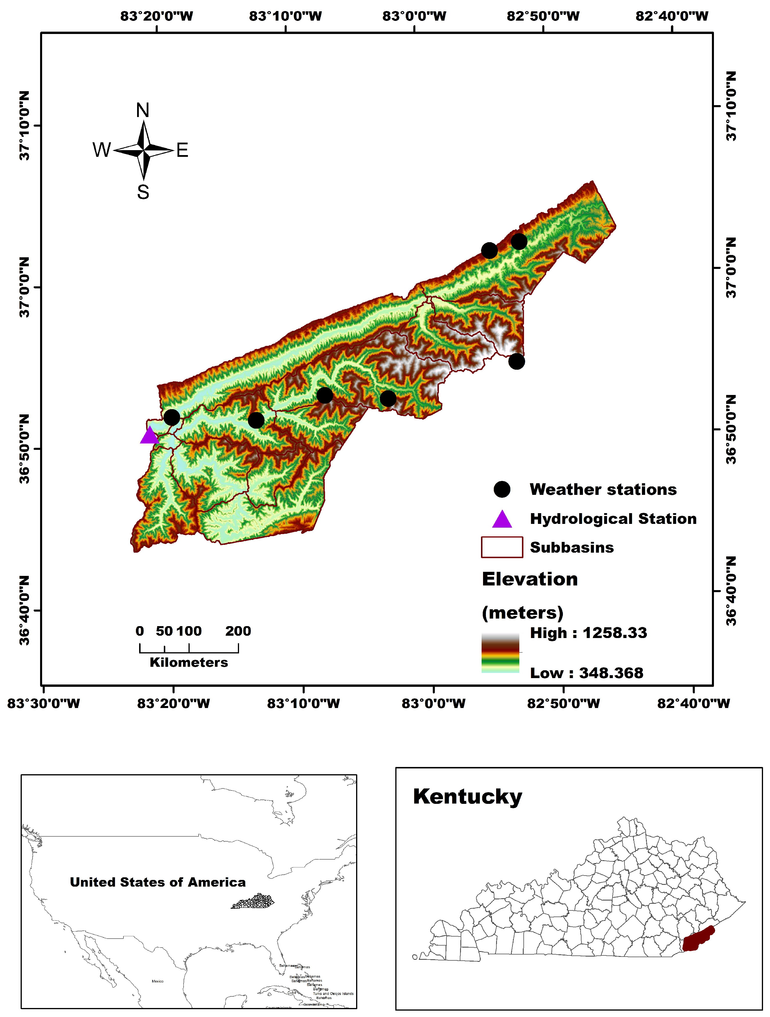
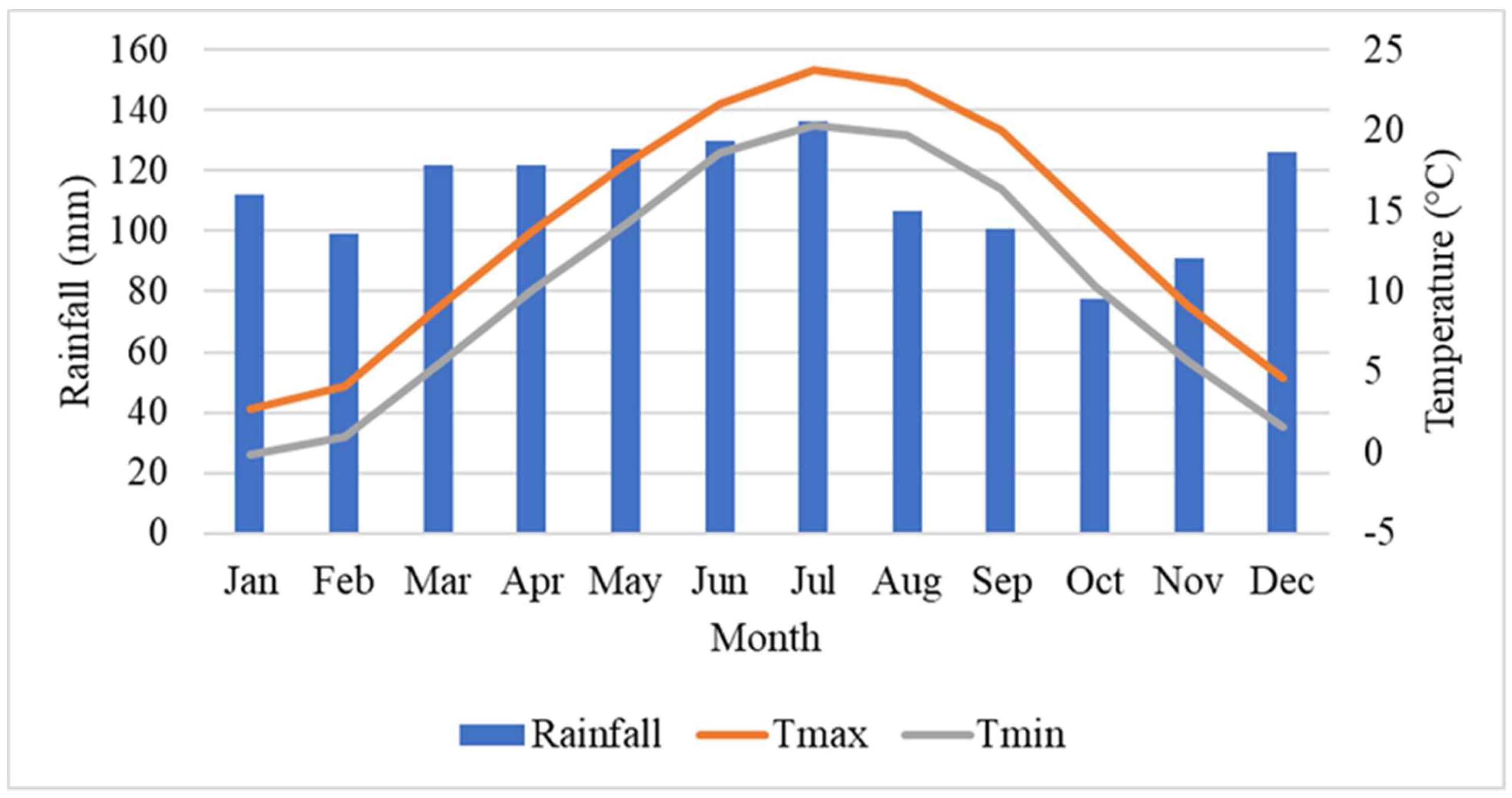
2.1. Study Site
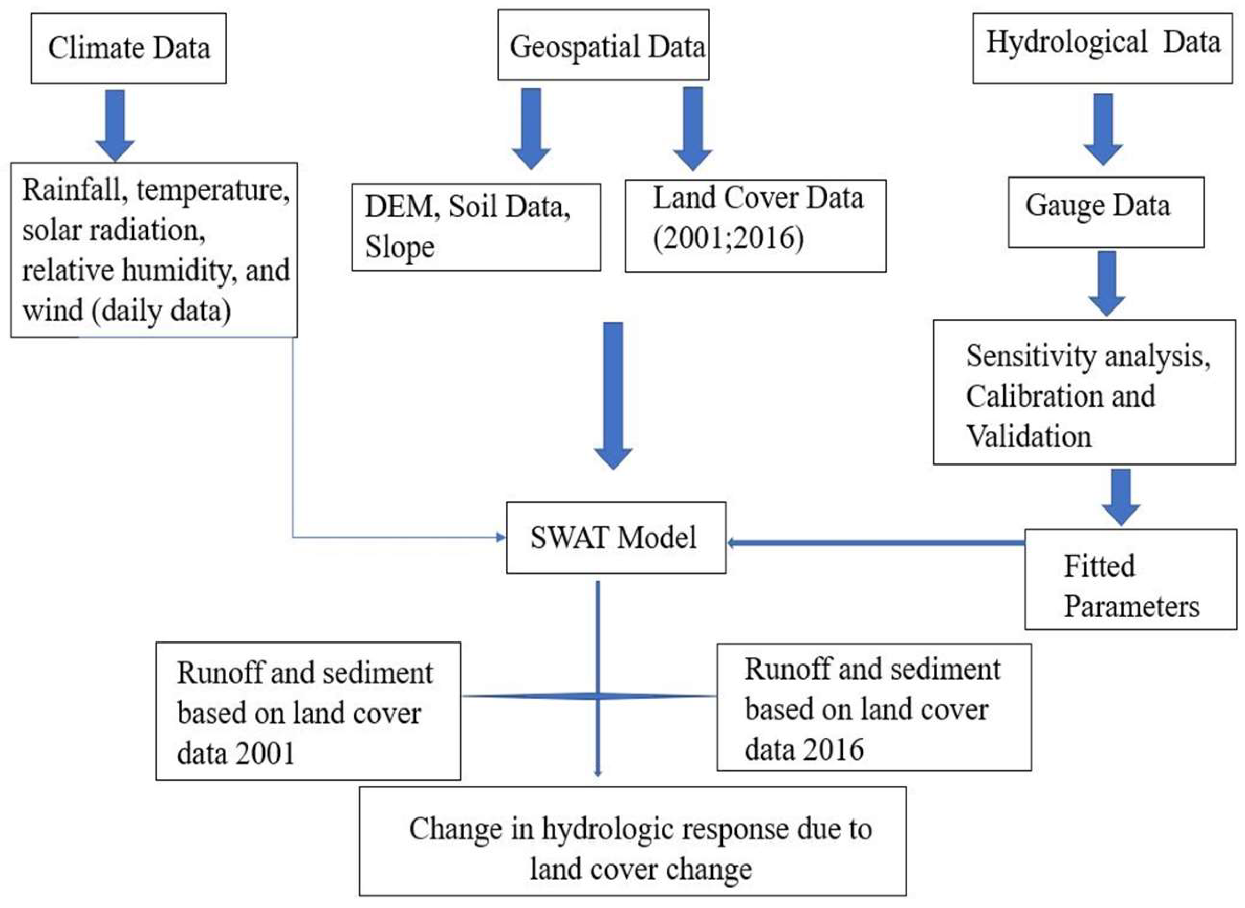
2.2. SWAT Model
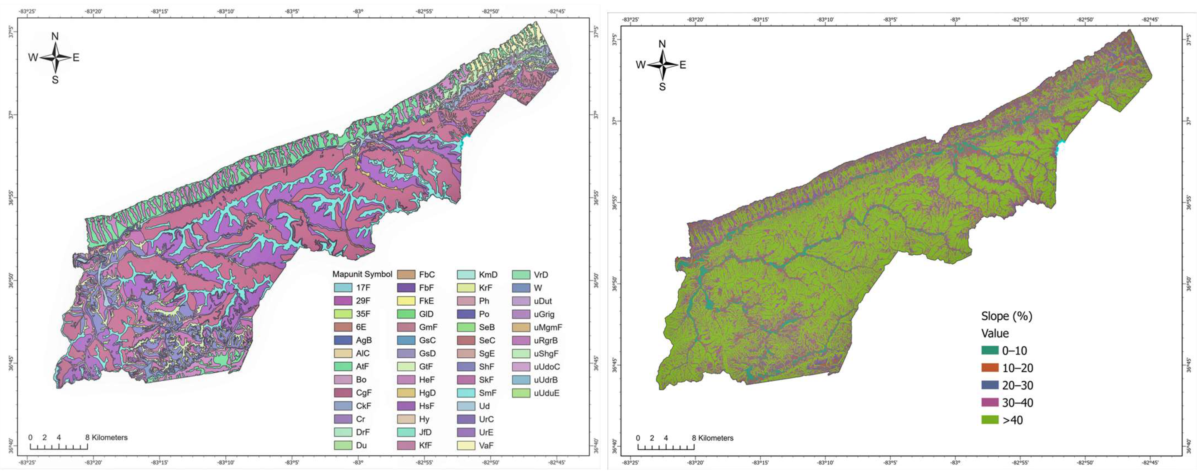
2.3. SWAT Input Data
2.4. SWAT Model Setup
2.5. Sensitivity Analysis
2.6. Model Calibration, Uncertainty Analysis, and Validation
3. Results
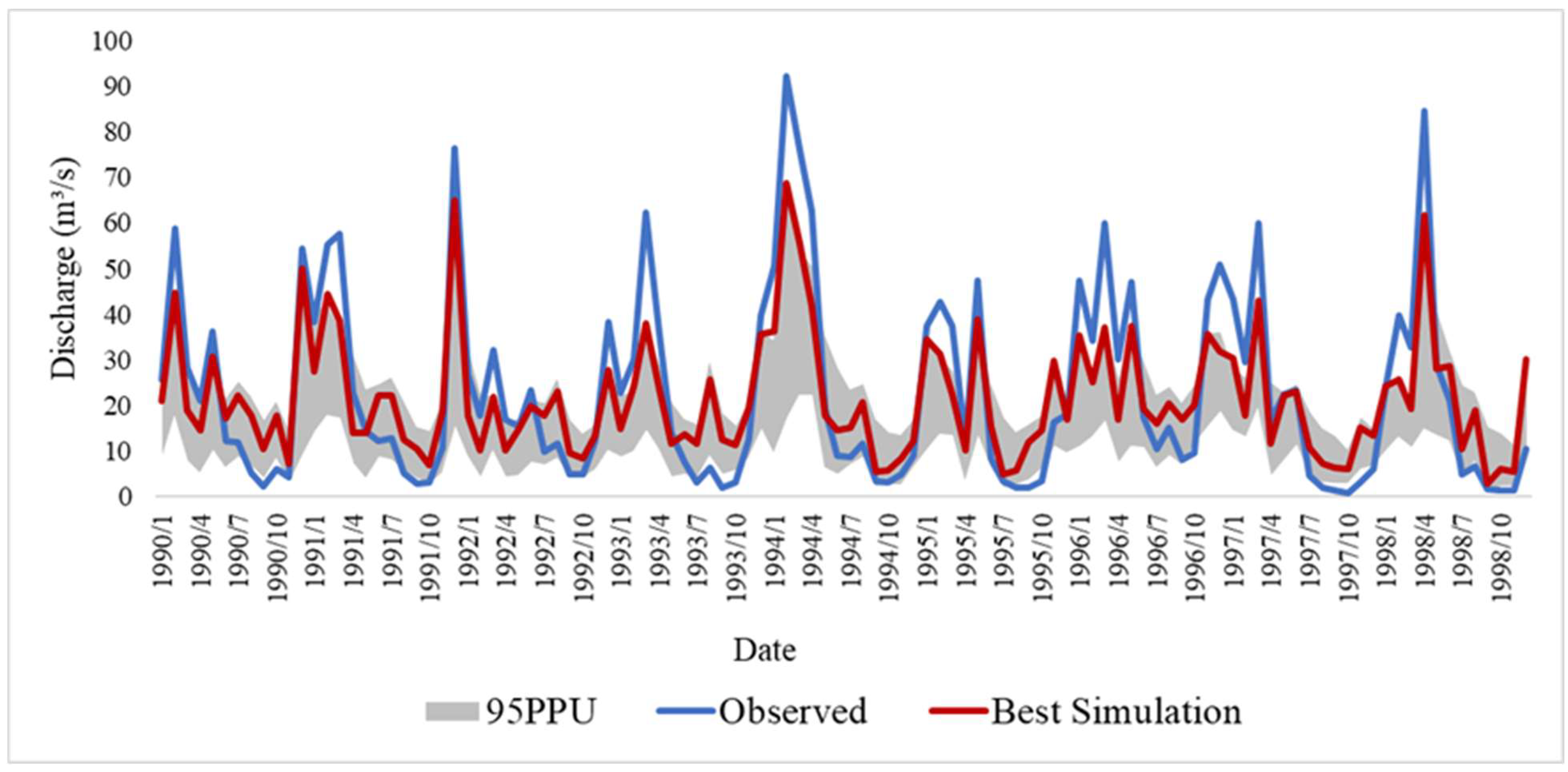
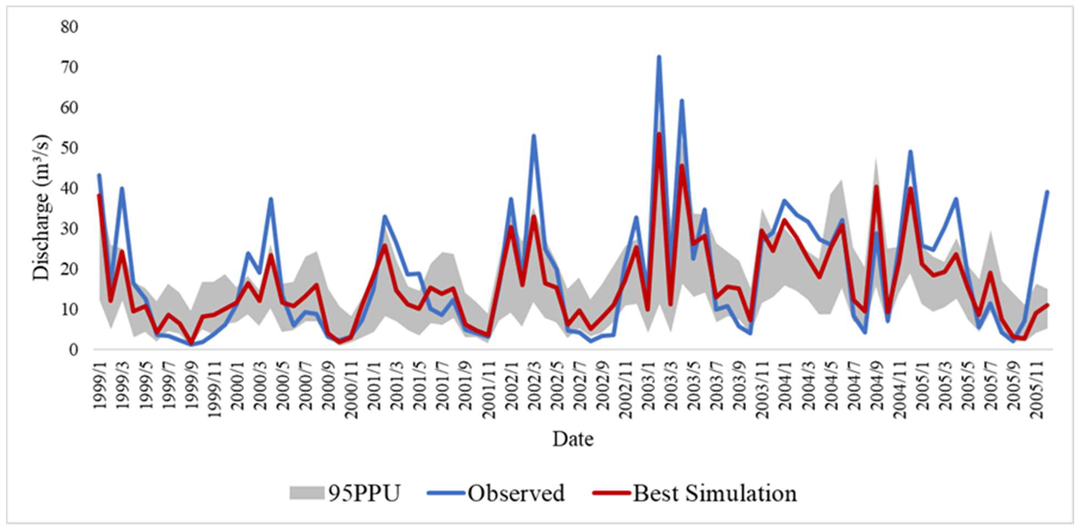
3.1. Calibration, Uncertainty, and Validation of Discharge
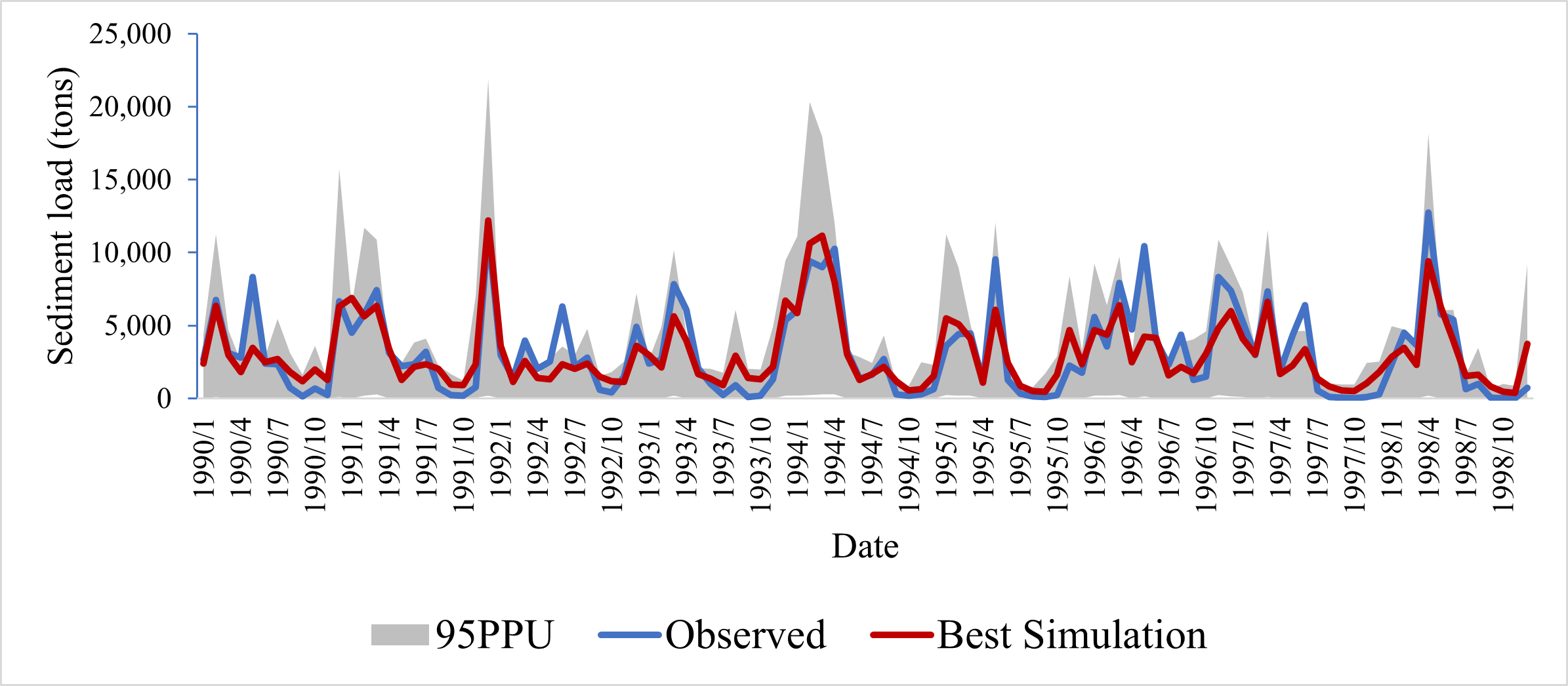
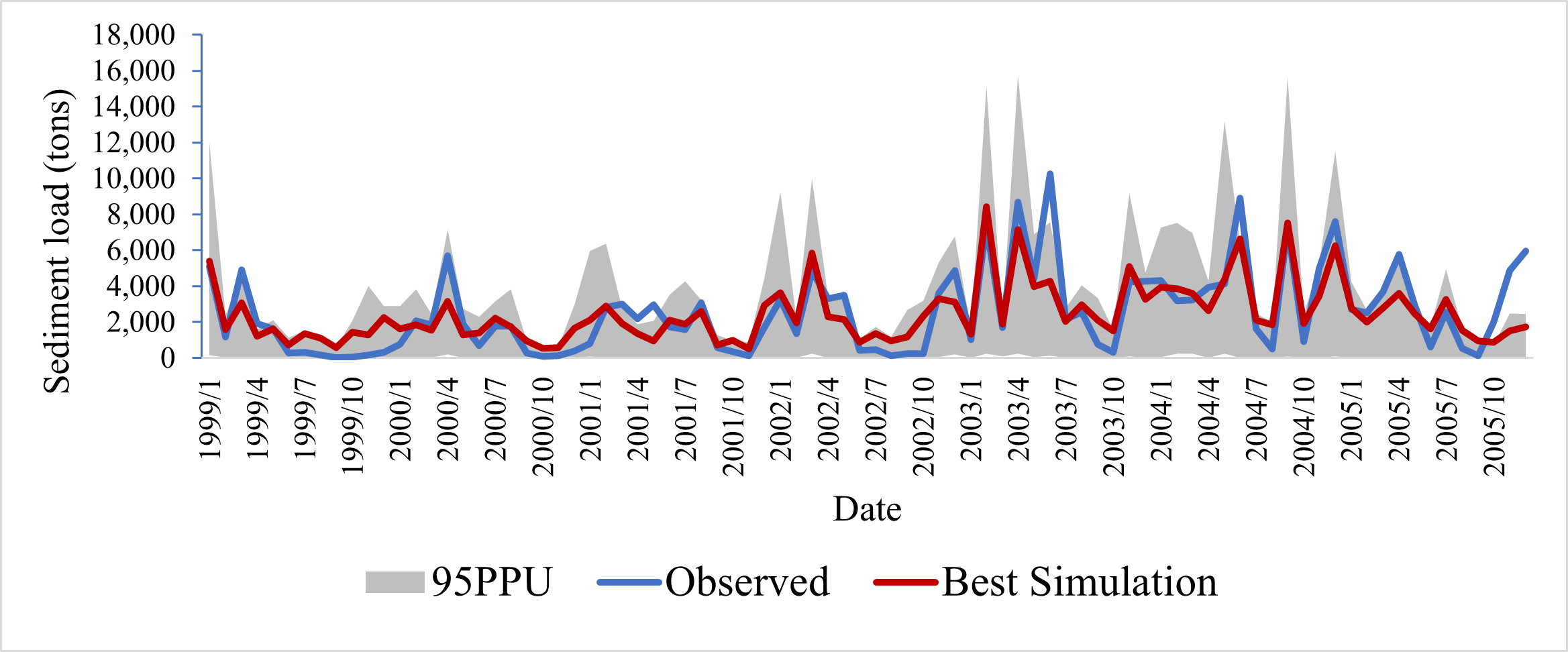
3.2. Calibration, Uncertainty, and Validation of Sediment
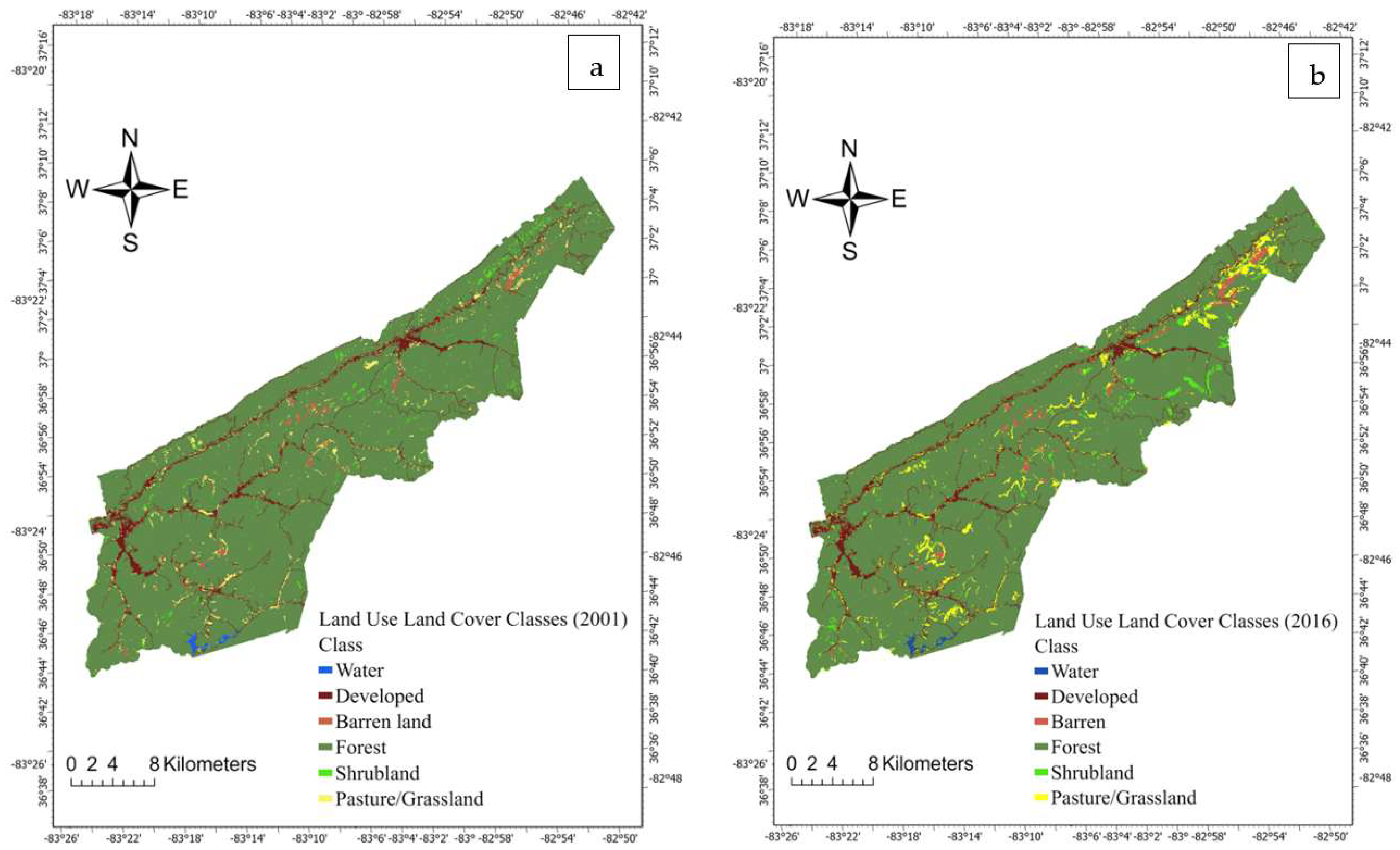
3.3. Land Use Land Cover Change Characteristics
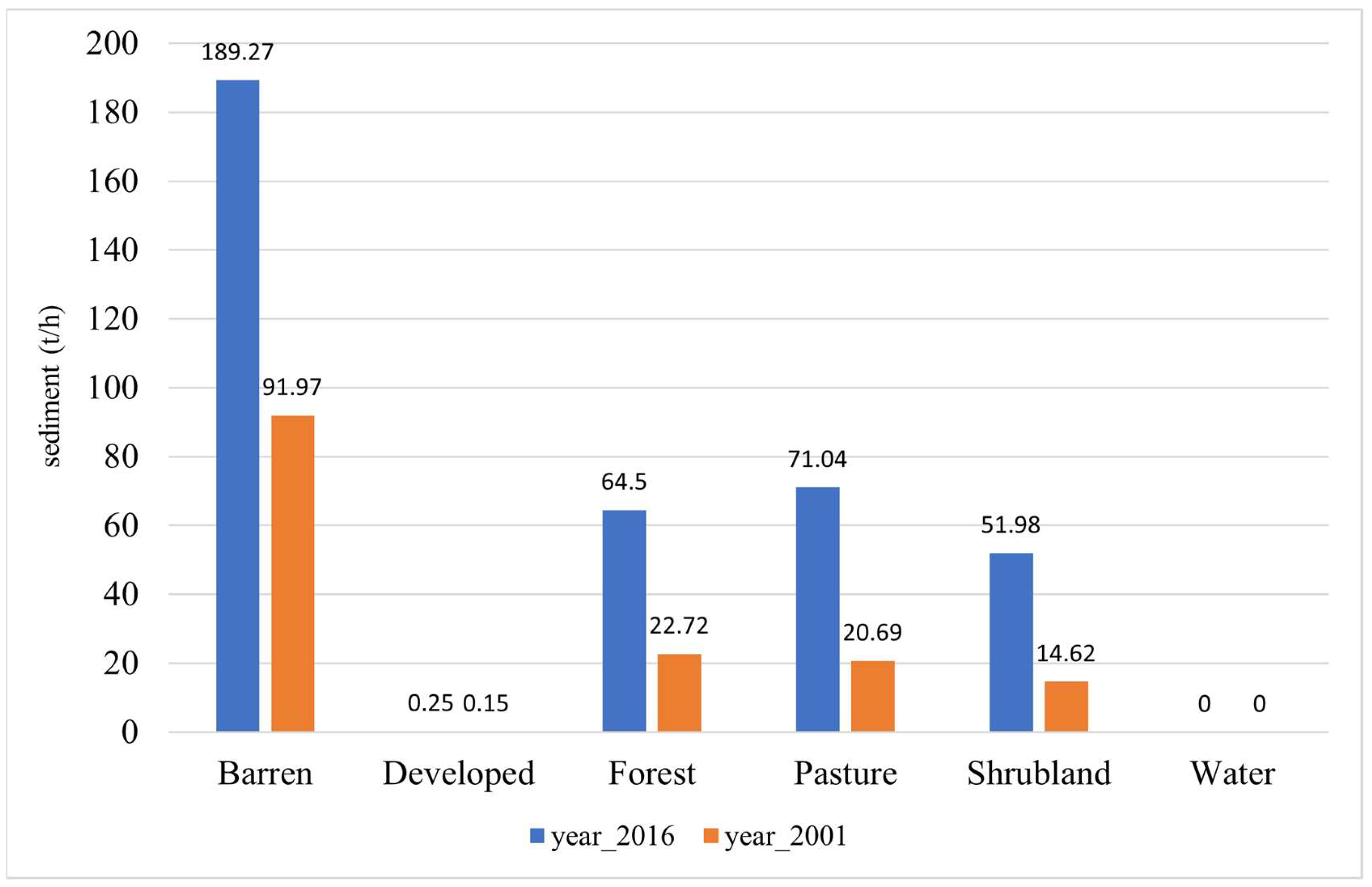
3.4. The Response of Discharge and Sediment under Different Land Cover Scenarios
4. Discussion
5. Conclusions
Author Contributions
Funding
Data Availability Statement
Acknowledgments
Conflicts of Interest
Patents
Declaration of Competing Interest
Appendix A. SSURGO Soil Class Descriptions

| Mapunit Symbol | Mapunit Name |
|---|---|
| 17F | Gilpin–Berks complex, 55 to 70 percent slopes |
| 29F | Gilpin–Summers–Kimper complex, 20 to 55 percent slopes, very stony |
| 35F | Wallen–Rock outcrop complex, 35 to 85 percent slopes, very stony |
| 6E | Bethesda, Fairpoint, and Sewell soils, 0 to 80 percent slopes, very rocky |
| AgB | Allegheny loam, 2 to 6 percent slopes |
| AlC | Allegheny loam, 2 to 15 percent slopes |
| AtF | Alticrest–Ramsey–Wallen complex, 20 to 55 percent slopes, rocky |
| Bo | Bonnie silt loam, occasionally flooded |
| CgF | Cloverlick–Guyandotte–Highsplint complex, 20 to 80 percent slopes, very stony |
| CkF | Cloverlick–Kimper–Highsplint complex, 30 to 65 percent slopes, very stony |
| Cr | Craigsville–Philo complex, occasionally flooded |
| DrF | Dekalb–Gilpin–Rayne complex, 25 to 65 percent slopes, very rocky |
| Du | Dumps, Mine; tailings; and Tipples |
| FbC | Fairpoint and Bethesda soils, 2 to 20 percent slopes |
| FbF | Fairpoint and Bethesda soils, 20 to 70 percent slopes, stony |
| FkE | Fiveblock and Kaymine soils, 0 to 30 percent slopes, stony |
| GlD | Gilpin–Shelocta complex, 12 to 25 percent slopes |
| GmF | Gilpin–Summers–Kimper complex, 20 to 55 percent slopes, very stony |
| GsC | Gilpin–Shelocta silt loams, 3 to 12 percent slopes |
| GsD | Gilpin–Shelocta silt loams, 12 to 20 percent slopes |
| GtF | Gilpin–Rayne–Sequoia complex, 25 to 55 percent slopes, very stony |
| HeF | Helechawa–Varilla–Jefferson complex, 35 to 75 percent slopes, very rocky |
| HgD | Highsplint very flaggy silt loam, 5 to 20 percent slopes, extremely bouldery |
| HsF | Highsplint–Shelocta–Dekalb complex, 35 to 80 percent slopes, very stony |
| Hy | Holly loam, frequently flooded |
| JfD | Jefferson gravelly silt loam, 12 to 20 percent slopes |
| KfF | Kaymine, Fairpoint, and Fiveblock soils, benched, 2 to 70 percent slopes, very stony |
| KmD | Kimper silt loam, 5 to 20 percent slopes, very stony |
| KrF | Kimper–Cloverlick–Renox complex, 30 to 80 percent slopes, extremely stony |
| Ph | Philo fine sandy loam, occasionally flooded |
| Po | Pope fine sandy loam, occasionally flooded |
| SeB | Shelocta gravelly silt loam, 2 to 6 percent slopes |
| SeC | Shelocta channery silt loam, 6 to 12 percent slopes |
| SgE | Shelocta–Gilpin silt loams, 20 to 35 percent slopes |
| ShF | Shelocta–Highsplint–Gilpin complex, 20 to 70 percent slopes, very stony |
| SkF | Shelocta–Kimper–Cloverlick complex, 20 to 80 percent slopes, very stony |
| SmF | Shelocta–Kimper–Cutshin complex, 20 to 55 percent slopes, very stony |
| Ud | Udorthents–Urban land complex, occasionally flooded |
| uDut | Dumps, mine, and tailings |
| uGrig | Grigsby fine sandy loam, 0 to 3 percent slopes, frequently flooded |
| uMgmF | Matewan–Gilpin–Marrowbone complex, 12 to 80 percent slopes, very rocky |
| UrC | Udorthents–Urban land complex, 3 to 15 percent slopes |
| UrE | Udorthents–Urban land complex, 15 to 35 percent slopes |
| uRgrB | Rowdy–Grigsby complex, 0 to 6 percent slopes, occasionally flooded |
| uShgF | Shelocta–Highsplint–Gilpin complex, 20 to 70 percent slopes, very stony |
| uUdoC | Udorthents–Urban land complex, 0 to 15 percent slopes |
| uUdrB | Udorthents–Urban land-Grigsby complex, 0 to 6 percent slopes, occasionally flooded |
| uUduE | Udorthents–Urban land-Rock outcrop complex, 0 to 35 percent slopes |
| VaF | Varilla–Jefferson–Alticrest complex, 35 to 75 percent slopes, very rocky |
| VrD | Varilla very stony loam, 5 to 20 percent slopes, extremely bouldery |
References
- NOAA. What Is a Watershed? 2020. Available online: https://oceanservice.noaa.gov/facts/watershed.html (accessed on 9 February 2020).
- NOAA. What Is the Difference between Land Cover and Land Use? 2021. Available online: https://oceanservice.noaa.gov/facts/lclu.html (accessed on 19 February 2021).
- Khoi, D.N.; Suetsugi, T. The responses of hydrological processes and sediment yield to land-use and climate change in the Be River Catchment, Vietnam. Hydrol. Process. 2014, 28, 640–652. [Google Scholar] [CrossRef]
- Bian, G.; Zhang, J.; Chen, J.; Wang, G.; Song, M. Spatial and seasonal variations of hydrological responses to climate and land-use changes in a highly urbanized basin of Southeastern China. Hydrol. Res. 2021, 52, 506–522. [Google Scholar] [CrossRef]
- Getachew, B.; Manjunatha, B.; Bhat, H.G. Modeling projected impacts of climate and land use/land cover changes on hydrological responses in the Lake Tana Basin, upper Blue Nile River Basin, Ethiopia. J. Hydrol. 2021, 595, 125974. [Google Scholar] [CrossRef]
- Aredo, M.R.; Hatiye, S.D.; Pingale, S.M. Impact of land use/land cover change on stream flow in the Shaya catchment of Ethiopia using the MIKE SHE model. Arab. J. Geosci. 2021, 14, 1–15. [Google Scholar] [CrossRef]
- Li, Z.; Liu, W.; Zhang, J.; Zheng, F.-L. Impacts of land use change and climate variability on hydrology in an agricultural catchment on the Loess Plateau of China. J. Hydrol. 2009, 377, 35–42. [Google Scholar] [CrossRef]
- Buendia, C.; Bussi, G.; Tuset, J.; Vericat, D.; Sabater, S.; Palau, A.; Batalla, R. Effects of afforestation on runoff and sediment load in an upland Mediterranean catchment. Sci. Total Environ. 2016, 540, 144–157. [Google Scholar] [CrossRef]
- Birkinshaw, S.J.; Guerreiro, S.B.; Nicholson, A.; Liang, Q.; Quinn, P.; Zhang, L.; He, B.; Yin, J.; Fowler, H.J. Climate change impacts on Yangtze River discharge at the Three Gorges Dam. Hydrol. Earth Syst. Sci. 2017, 21, 1911–1927. [Google Scholar] [CrossRef] [Green Version]
- Yonaba, R.; Biaou, A.C.; Koïta, M.; Tazen, F.; Mounirou, L.A.; Zouré, C.O.; Queloz, P.; Karambiri, H.; Yacouba, H. A dynamic land use/land cover input helps in picturing the Sahelian paradox: Assessing variability and attribution of changes in surface runoff in a Sahelian watershed. Sci. Total. Environ. 2020, 757, 143792. [Google Scholar] [CrossRef]
- Turner, B.L., II; Lambin, E.F.; Reenberg, A. The emergence of land change science for global environmental change and sustainability. Proc. Natl. Acad. Sci. USA 2007, 104, 20666–20671. [Google Scholar] [CrossRef] [Green Version]
- Mi, J.; Yang, Y.; Zhang, S.; An, S.; Hou, H.; Hua, Y.; Chen, F. Tracking the Land Use/Land Cover Change in an Area with Underground Mining and Reforestation via Continuous Landsat Classification. Remote Sens. 2019, 11, 1719. [Google Scholar] [CrossRef]
- Höök, M.; Aleklett, K. Historical trends in American coal production and a possible future outlook. Int. J. Coal Geol. 2009, 78, 201–216. [Google Scholar] [CrossRef]
- Turner, M.G.; Ruscher, C.L. Changes in landscape patterns in Georgia, USA. Landsc. Ecol. 1988, 1, 241–251. [Google Scholar] [CrossRef]
- USEPA. The Effects of Mountaintop Mines and Valley Fills on Aquatic Ecosystems of the Central Appalachian Coalfields; EPA/600/R-09/138F; USEPA: Washington, DC, USA, 2011. Available online: https://cfpub.epa.gov/ncea/risk/recordisplay.cfm?deid=225743 (accessed on 17 March 2020).
- Bajocco, S.; De Angelis, A.; Perini, L.; Ferrara, A.; Salvati, L. The Impact of Land Use/Land Cover Changes on Land Degradation Dynamics: A Mediterranean Case Study. Environ. Manag. 2012, 49, 980–989. [Google Scholar] [CrossRef] [PubMed]
- Tadesse, L.; Suryabhagavan, K.; Sridhar, G.; Legesse, G. Land use and land cover changes and Soil erosion in Yezat Watershed, North Western Ethiopia. Int. Soil Water Conserv. Res. 2017, 5, 85–94. [Google Scholar] [CrossRef] [Green Version]
- Hooke, R.L. Spatial distribution of human geomorphic activity in the United States: Comparison with rivers. Earth Surf. Process. Landforms 1999, 24, 687–692. [Google Scholar] [CrossRef]
- Huang, Y.; Tian, F.; Wang, Y.; Wang, M.; Hu, Z. Effect of coal mining on vegetation disturbance and associated carbon loss. Environ. Earth Sci. 2014, 73, 2329–2342. [Google Scholar] [CrossRef]
- Ross, M.R.V.; McGlynn, B.L.; Bernhardt, E.S. Deep Impact: Effects of Mountaintop Mining on Surface Topography, Bedrock Structure, and Downstream Waters. Environ. Sci. Technol. 2016, 50, 2064–2074. [Google Scholar] [CrossRef] [Green Version]
- California Department of Conservation. 2019. Available online: https://www.conservation.ca.gov/dmr/SMARA%20Mines/reclamation (accessed on 17 March 2018).
- Wang, C.; Lv, Y.; Song, Y. Researches on mining subsidence disaster management GIS’s system. In Proceedings of the 2012 International Conference on Systems and Informatics (ICSAI2012), Yantai, China, 19–20 May 2012; pp. 2493–2496. [Google Scholar] [CrossRef]
- Eastern Kentucky Coalfield. Wikipedia. 2021. Available online: https://en.wikipedia.org/wiki/Eastern_Kentucky_Coalfield (accessed on 15 January 2021).
- Gurung, K.; Yang, J.; Fang, L. Assessing Ecosystem Services from the Forestry-Based Reclamation of Surface Mined Areas in the North Fork of the Kentucky River Watershed. Forests 2018, 9, 652. [Google Scholar] [CrossRef] [Green Version]
- Bai, Y.; Ochuodho, T.O.; Yang, J. Impact of land use and climate change on water-related ecosystem services in Kentucky, USA. Ecol. Indic. 2019, 102, 51–64. [Google Scholar] [CrossRef]
- Kentucky Division of Water. Kentucky Nonpoint Source Management Plan: A Strategy for 2019–2023. 2019. Available online: https://services.statescape.com/ssu/Regs/ss_8586430572245812376.pdf (accessed on 15 January 2021).
- Kentucky Geological Survey. Water Fact Sheet. 2021. Available online: https://www.uky.edu/KGS/water/ (accessed on 9 February 2020).
- Phillips, J.D. Impacts of surface mine valley fills on headwater floods in eastern Kentucky. Environ. Earth Sci. 2004, 45, 367–380. [Google Scholar] [CrossRef]
- Negley, T.L.; Eshleman, K.N. Comparison of stormflow responses of surface-mined and forested watersheds in the Appalachian Mountains, USA. Hydrol. Process. 2006, 20, 3467–3483. [Google Scholar] [CrossRef]
- Evans, D.M.; Zipper, C.E.; Hester, E.T.; Schoenholtz, S.H. Hydrologic effects of surface coal mining in Appalachia (US). J. Am. Water Resour. Assoc. 2015, 51, 1436–1452. [Google Scholar] [CrossRef]
- Clark, E.V.; Zipper, C.E.; Soucek, D.J.; Daniels, W.L. Contaminants in Appalachian water resources generated by non-acid-forming coal-mining materials. In Appalachia’s Coal Mined Landscapes; Chapter 9; Zipper, C.E., Skousen, J.G., Eds.; Springer: Berlin/Heidelberg, Germany, 2021. [Google Scholar]
- Arnold, J.G.; Srinivasan, R.; Muttiah, R.S.; Williams, J.R. Large area hydrologic modeling and assessment part I: Model development 1. J. Am. Water Resour. Assoc. 1998, 34, 73–89. [Google Scholar] [CrossRef]
- Pokhrel, B.K. Impact of Land Use Change on Flow and Sediment Yields in the Khokana Outlet of the Bagmati River, Kathmandu, Nepal. Hydrology 2018, 5, 22. [Google Scholar] [CrossRef] [Green Version]
- Shang, X.; Jiang, X.; Jia, R.; Wei, C. Land Use and Climate Change Effects on Surface Runoff Variations in the Upper Heihe River Basin. Water 2019, 11, 344. [Google Scholar] [CrossRef] [Green Version]
- Zhang, S.; Li, Z.; Hou, X.; Yi, Y. Impacts on watershed-scale runoff and sediment yield resulting from synergetic changes in climate and vegetation. CATENA 2019, 179, 129–138. [Google Scholar] [CrossRef]
- Kateb, Z.; Bouchelkia, H.; Benmansour, A.; Belarbi, F. Sediment transport modeling by the SWAT model using two scenarios in the watershed of Beni Haroun dam in Algeria. Arab. J. Geosci. 2020, 13, 1–17. [Google Scholar] [CrossRef]
- Sinha, R.K.; Eldho, T.I.; Subimal, G. Assessing the impacts of land cover and climate on runoff and sediment yield of a river basin. Hydrol. Sci. J. 2020, 65, 2097–2115. [Google Scholar] [CrossRef]
- Aboelnour, M.; Gitau, M.W.; Engel, B.A. Hydrologic Response in an Urban Watershed as Affected by Climate and Land-Use Change. Water 2019, 11, 1603. [Google Scholar] [CrossRef]
- Spruill, C.A.; Workman, S.R.; Taraba, J.L. Simulation of daily stream discharge from small watersheds using the SWAT model. Am. Soc. Agric. Biol. Eng. 2000, 1, 1431–1439. [Google Scholar] [CrossRef]
- SWAT Literature Database. Available online: https://www.card.iastate.edu/swat_articles/ (accessed on 15 May 2021).
- Gyawali, B.; Shrestha, S.; Bhatta, A.; Pokhrel, B.; Cristan, R.; Antonious, G.; Banerjee, S.; Paudel, K.P. Assessing the Effect of Land-Use and Land-Cover Changes on Discharge and Sediment Yield in a Rural Coal-Mine Dominated Watershed in Kentucky, USA. Water 2022, 14, 516. [Google Scholar] [CrossRef]
- U.S. Census Bureau. QuickFacts Harlan County, Kentucky. 2020. Available online: https://www.census.gov/quickfacts/harlancountykentucky (accessed on 17 March 2020).
- Srinivasan, R.; Arnold, J.G. Integration of A Basin-Scale Water Quality Model With Gis. JAWRA J. Am. Water Resour. Assoc. 1994, 30, 453–462. [Google Scholar] [CrossRef]
- Arnold, J.G.; Moriasi, D.N.; Gassman, P.W.; Abbaspour, K.C.; White, M.J.; Srinivasan, R.; Santhi, C.; Harmel, R.D.; van Griensven, A.; Van Liew, M.W.; et al. SWAT: Model Use, Calibration, and Validation. Trans. ASABE 2012, 55, 1491–1508. [Google Scholar] [CrossRef]
- Zhang, P.; Liu, R.; Bao, Y.; Wang, J.; Yu, W.; Shen, Z. Uncertainty of SWAT model at different DEM resolutions in a large mountainous watershed. Water Res. 2014, 53, 132–144. [Google Scholar] [CrossRef] [PubMed]
- Zhang, Y.; Su, F.; Hao, Z.; Xu, C.; Yu, Z.; Wang, L.; Tong, K. Impact of projected climate change on the hydrology in the headwaters of the Yellow River basin. Hydrol. Process. 2015, 29, 4379–4397. [Google Scholar] [CrossRef]
- Neitsch, S.L.; Arnold, J.G.; Kiniry, J.R.; Williams, J.R. Soil and Water Assessment Tool Theoretical Documentation Version 2009; Texas Water Resources Institute: College Station, TX, USA, 2011. [Google Scholar]
- Williams, J.R.; Berndt, H.D. Sediment Yield Prediction Based on Watershed Hydrology. Trans. ASAE 1977, 20, 1100–1104. [Google Scholar] [CrossRef]
- Runkel, R.L.; Crawford, C.G.; Cohn, T.A. Load estimator (LOADEST): A FORTRAN program for estimating constituent loads in streams and rivers. In USGS Techniques and Methods; USGS Numbered Series No. 4-A5; USGS: Reston, VA, USA, 2004. [Google Scholar]
- Abbaspour, K.C. SWAT-CUP Premium 2020: SWAT Calibration and Uncertainty Programs (Premium Versions): A User Manual. 2020. Available online: https://swat.tamu.edu/media/114860/usermanual_swatcup.pdf (accessed on 23 October 2020).
- Servat, E.; Dezetter, A. Selection of calibration objective fonctions in the context of rainfall-ronoff modelling in a Sudanese savannah area. Hydrol. Sci. J. 1991, 36, 307–330. [Google Scholar] [CrossRef]
- Sao, D.; Kato, T.; Tu, L.H.; Thouk, P.; Fitriyah, A.; Oeurng, C. Evaluation of Different Objective Functions Used in the SUFI-2 Calibration Process of SWAT-CUP on Water Balance Analysis: A Case Study of the Pursat River Basin, Cambodia. Water 2020, 12, 2901. [Google Scholar] [CrossRef]
- Moriasi, D.N.; Gitau, M.W.; Pai, N.; Daggupati, P. Hydrologic and Water Quality Models: Performance Measures and Evaluation Criteria. Trans. ASABE 2015, 58, 1763–1785. [Google Scholar] [CrossRef]
- Abbaspour, K.C.; Yang, J.; Maximov, I.; Siber, R.; Bogner, K.; Mieleitner, J.; Zobrist, J.; Srinivasan, R. Modelling hydrology and water quality in the pre-alpine/alpine Thur watershed using SWAT. J. Hydrol. 2007, 333, 413–430. [Google Scholar] [CrossRef]
- Abbaspour, K.C.; Rouholahnejad, E.; Vaghefi, S.; Srinivasan, R.; Yang, H.; Kløve, B. A continental-scale hydrology and water quality model for Europe: Calibration and uncertainty of a high-resolution large-scale SWAT model. J. Hydrol. 2015, 524, 733–752. [Google Scholar] [CrossRef] [Green Version]
- Abbaspour, K.C.; Vaghefi, S.A.; Srinivasan, R. A Guideline for Successful Calibration and Uncertainty Analysis for Soil and Water Assessment: A Review of Papers from the 2016 International SWAT Conference. Water 2017, 10, 6. [Google Scholar] [CrossRef] [Green Version]
- Moriasi, D.N.; Arnold, J.G.; van Liew, M.W.; Bingner, R.L.; Harmel, R.D.; Veith, T.L. Model evaluation guidelines for systematic quantification of accuracy in watershed simulations. Trans. ASABE 2007, 50, 885–900. [Google Scholar] [CrossRef]
- Santhi, C.; Arnold, J.G.; Williams, J.R.; Dugas, W.A.; Srinivasan, R.; Hauck, L.M. Validation of the Swat Model on A Large Rwer Basin with Point and Nonpoint Sources. J. Am. Water Resour. Assoc. 2001, 37, 1169–1188. [Google Scholar] [CrossRef]
- Van Liew, M.W.; Arnold, J.G.; Garbrecht, J.D. Hydrologic Simulation on Agricultural Watersheds: Choosing between Two Models. Trans. ASAE 2003, 46, 1539–1551. [Google Scholar] [CrossRef]
- Narsimlu, B.; Gosain, A.K.; Chahar, B.R.; Singh, S.K.; Srivastava, P.K. SWAT Model Calibration and Uncertainty Analysis for Streamflow Prediction in the Kunwari River Basin, India, Using Sequential Uncertainty Fitting. Environ. Process. 2015, 2, 79–95. [Google Scholar] [CrossRef]
- Mapes, K.L.; Pricope, N.G. Evaluating SWAT Model Performance for Runoff, Percolation, and Sediment Loss Estimation in Low-Gradient Watersheds of the Atlantic Coastal Plain. Hydrology 2020, 7, 21. [Google Scholar] [CrossRef] [Green Version]
- Tang, F.; Xu, H.; Xu, Z. Model calibration and uncertainty analysis for runoff in the Chao River Basin using sequential uncertainty fitting. Procedia Environ. Sci. 2012, 13, 1760–1770. [Google Scholar] [CrossRef] [Green Version]
- Briak, H.; Moussadek, R.; Aboumaria, K.; Mrabet, R. Assessing sediment yield in Kalaya gauged watershed (Northern Morocco) using GIS and SWAT model. Int. Soil Water Conserv. Res. 2016, 4, 177–185. [Google Scholar] [CrossRef]
- Jha, M.; Gassman, P.W.; Secchi, S.; Arnold, J. Upper Mississippi River Basin modeling system part 2: Baseline simulation results. In Coastal Hydrology and Processes; Water Resources Publications: Highland Ranch, CO, USA, 2006. [Google Scholar]
- Schmalz, B.; Fohrer, N. Comparing model sensitivities of different landscapes using the ecohydrological SWAT model. Adv. Geosci. 2009, 21, 91–98. [Google Scholar] [CrossRef] [Green Version]
- Ngo, T.S.; Nguyen, D.B.; Rajendra, P.S. Effect of land use change on runoff and sediment yield in Da River Basin of Hoa Binh province, Northwest Vietnam. J. Mt. Sci. 2015, 12, 1051–1064. [Google Scholar] [CrossRef]
- Zhu, C. Land Use/Land Cover Change and Its Hydrological Impacts from 1984 to 2010 in the Little River Watershed, Tennessee. Int. Soil Water Conserv. Res. 2014, 2, 11–21. [Google Scholar] [CrossRef] [Green Version]
- Hovenga, P.A.; Wang, D.; Medeiros, S.C.; Hagen, S.C.; Alizad, K. The response of runoff and sediment loading in the Apalachicola River, Florida to climate and land use land cover change. Earth’s Futur. 2016, 4, 124–142. [Google Scholar] [CrossRef]


| Data | Measurable Unit | Spatial Unit | Year | Source |
|---|---|---|---|---|
| Digital Elevation Model (DEM) | Pixel level | 30 m × 30 m resolution | 2020 | https://kygeoportal.ky.gov/ (accessed on 12 April 2020). |
| Soil (Physical properties) | Shapefile | 2020 | USDA (SSURGO) www.nrcs.usda.gov (accessed on 12 April 2020) | |
| Land cover | Pixel level | 30 m × 30 m resolution | 2001 and 2016 | Multi-Resolution Land Cover Characteristics (MRLC) Consortium, https://www.mrlc.gov/ (accessed on 12 April 2020) |
| Meteorological (rainfall, solar radiation, temperature, humidity, wind velocity) | Table, txt | Daily data | 1987–2016 | Prism Climate Group https://prism.oregonstate.edu/ (accessed on 20 April 2020), Global weather Data for SWAT https://globalweather.tamu.edu/ |
| Discharge | Monthly (m3/s) | 1990–2005 | https://waterdata.usgs.gov/nwis (accessed on 15 April 2020) | |
| Sediment | Monthly (ton/ha) | 1990–2005 | https://waterdata.usgs.gov/nwis (accessed on 15 April 2020), LOADEST |
| Parameters | Definition | Unit | Default Range of Values | Values Set in SWAT-CUPP |
|---|---|---|---|---|
| Parameters for Discharge | ||||
| r__CN2.mgt | SCS runoff curve number for moisture condition II | - | 35 to 98 | −0.4 to 0.5 |
| r__SOL_K().sol | Saturated hydraulic conductivity | mm/hr | 0 to 2000 | −0.5 to 0.5 |
| r__SOL_AWC().sol | Available water capacity of the soil layer | mm H2O/mm soil | 0 to 1 | −0.5 to 0.5 |
| r__SOL_BD().sol | Moist bulk density | Mg/m3 or g/cm3 | 0.9 to 2.5 | −0.5 to 0.5 |
| v__CH_K2.rte | Effective hydraulic conductivity in main channel alluvium | mm/hr | −0.01 to 500 | −0.01 to 500 |
| r__HRU_SLP.hru | Average slope steepness | m/m | 0 to 0.6 | −0.5 to 0.5 |
| v__RCHRG_DP.gw | Deep aquifer percolation fraction | - | 0 to 1 | 0 to 1 |
| v__GWQMN.gw | Threshold depth of water in the shallow aquifer required for return flow to occur | mm H2O | 0 to 5000 | 0 to 5000 |
| v__ESCO.hru | Soil evaporation compensation factor | - | 0 to 1 | −0.5 to 0.5 |
| r__SLSUBBSN.hru | Average slope length. | m | 10 to 150 | −0.5 to 0.5 |
| v__GW_DELAY.gw | Groundwater delay | days | 0 to 500 | 0 to 500 |
| v__GW_REVAP.gw | Groundwater “revap” coefficient. | - | 0.02 to 0.2 | 0.02 to 0.2 |
| v__REVAPMN.gw | Threshold depth of water in the shallow aquifer for “revap” to occur (mm). | mm | 0 to 1000 | 0 to 1000 |
| v__ALPHA_BF.gw | Baseflow alpha factor (days) | days | 0 to 1 | 0 to 1 |
| r__OV_N.hru | Manning’s “n” value for overland flow | - | 0.01 to 4 | −0.5 to 0.5 |
| v__SURLAG.bsn | Surface runoff lag time | - | 0.05 to 24 | 0.05 to 24 |
| v__CH_N2.rte | Manning’s “n” value for the main channel | - | −0.01 to 0.3 | −0.01 to 0.3 |
| Parameters for sediment | ||||
| v__PRF.bsn | Peak rate adjustment factor for sediment routing in the main channel | 0 to 2 | 0 to 2 | |
| v__SPCON.bsn | Linear parameter for calculating the maximum amount of sediment that can be re-entrained during channel sediment routing | - | 0.0001 to 0.01 | 0.0001 to 0.01 |
| v__SPEXP.bsn | Exponent parameter for calculating sediment re-entrained in channel sediment routing | - | 1 to 1.5 | 1 to 1.5 |
| v__CH_COV1.rte | Channel erodibility factor | - | −0.001 to 1 | −0.05 to 0.6 |
| v__USLE_K.sol | USLE equation soil erodibility (K) factor | (metric ton m2 hr)/(m3-metric ton cm) | 0 to 0.65 | 0 to 0.65 |
| Parameters | Fitted Value | p-Value | t-Stat | Ranking |
|---|---|---|---|---|
| v__ALPHA_BF.gw | 0.57 | 0.0 | 15.22 | 1 |
| r__CN2.mgt | 0.39 | 0.0 | 9.57 | 2 |
| r__SOL_BD().sol | 0.46 | 0.0 | 7.33 | 3 |
| r__SOL_K().sol | −0.25 | 0.0000025 | 4.74 | 4 |
| v__RCHRG_DP.gw | 0.50 | 0.0000056 | 4.58 | 5 |
| r__HRU_SLP.hru | −0.35 | 0.000086 | 3.95 | 6 |
| r__SOL_AWC().sol | −0.40 | 0.0001 | −3.91 | 7 |
| v__ESCO.hru | 0.30 | 0.00022 | 3.70 | 8 |
| v__CH_N2.rte | 0.009 | 0.0018 | −3.13 | 9 |
| v__CH_K2.rte | 129.49 | 0.0039 | −2.89 | 10 |
| v__GWQMN.gw | 1695.83 | 0.005 | −2.81 | 11 |
| r__OV_N.hru | −0.21 | 0.52 | 0.62 | 12 |
| v__REVAPMN.gw | 684.16 | 0.64 | −0.46 | 13 |
| v__SURLAG.bsn | 3.66 | 0.75 | −0.31 | 14 |
| v__GW_REVAP.gw | 0.03 | 0.81 | −0.22 | 15 |
| r__EPCO.hru | 0.49 | 0.83 | 0.20 | 16 |
| r__SLSUBBSN.hru | 0.16 | 0.89 | −0.13 | 17 |
| v__GW_DELAY.gw | 79.58 | 0.91 | 0.11 | 18 |
| Calibration/Validation | Criteria | Value |
|---|---|---|
| Calibration (1990–1998) | NSE | 0.76 |
| R2 | 0.85 | |
| PBIAS | 5.4 | |
| RSR | 0.49 | |
| P-factor | 0.5 | |
| R-factor | 0.83 | |
| Validation (1999–2005) | NSE | 0.74 |
| R2 | 0.8 | |
| PBIAS | 12.2 | |
| RSR | 0.51 | |
| P-factor | 0.62 | |
| R-factor | 1.04 |
| Calibration/Validation | Criteria | Value |
|---|---|---|
| Calibration (1990–1998) | NSE | 0.74 |
| R2 | 0.75 | |
| PBIAS | 5.9 | |
| RSR | 0.51 | |
| P-factor | 0.91 | |
| R-factor | 1.6 | |
| Validation (1999–2005) | NSE | 0.67 |
| R2 | 0.68 | |
| PBIAS | 2.8 | |
| RSR | 0.57 | |
| P-factor | 0.9 | |
| R-factor | 1.79 |
| Land Cover Class | 2001 | 2016 | % Difference |
|---|---|---|---|
| Area (%) | Area (%) | ||
| Water | 0.2 | 0.2 | −0.01 |
| Developed | 5.5 | 5.6 | 0.1 |
| Barren | 1.0 | 1.3 | 0.3 |
| Forest | 90.0 | 87.1 | −2.4 |
| Shrubland | 1.0 | 1.6 | 0.5 |
| Pasture/Grassland | 2.4 | 3.9 | 1.4 |
| Total | 100 | 100 |
| Component | Land Cover | ||
|---|---|---|---|
| 2001 | 2016 | %Change | |
| Surface Runoff (mm) | 92.3 | 104.7 | 11.8 |
| Sediment Yield (t/ha) | 0.8 | 1.63 | 49.0 |
| Potential Evapotranspiration (mm) | 595.5 | 607.4 | 1.9 |
| Lateral Flow (mm) | 541.6 | 562.6 | 3.7 |
Disclaimer/Publisher’s Note: The statements, opinions and data contained in all publications are solely those of the individual author(s) and contributor(s) and not of MDPI and/or the editor(s). MDPI and/or the editor(s) disclaim responsibility for any injury to people or property resulting from any ideas, methods, instructions or products referred to in the content. |
© 2023 by the authors. Licensee MDPI, Basel, Switzerland. This article is an open access article distributed under the terms and conditions of the Creative Commons Attribution (CC BY) license (https://creativecommons.org/licenses/by/4.0/).
Share and Cite
Kandel, S.; Gyawali, B.; Shrestha, S.; Zourarakis, D.; Antonious, G.; Gebremedhin, M.; Pokhrel, B. Estimation of Runoff and Sediment Yield in Response to Temporal Land Cover Change in Kentucky, USA. Land 2023, 12, 147. https://doi.org/10.3390/land12010147
Kandel S, Gyawali B, Shrestha S, Zourarakis D, Antonious G, Gebremedhin M, Pokhrel B. Estimation of Runoff and Sediment Yield in Response to Temporal Land Cover Change in Kentucky, USA. Land. 2023; 12(1):147. https://doi.org/10.3390/land12010147
Chicago/Turabian StyleKandel, Smriti, Buddhi Gyawali, Sandesh Shrestha, Demetrio Zourarakis, George Antonious, Maheteme Gebremedhin, and Bijay Pokhrel. 2023. "Estimation of Runoff and Sediment Yield in Response to Temporal Land Cover Change in Kentucky, USA" Land 12, no. 1: 147. https://doi.org/10.3390/land12010147